Non-ergodicity of the motion in three dimensional steep repelling dispersing potentials.

Abstract

It is demonstrated numerically that smooth three degrees of freedom Hamiltonian systems which are arbitrarily close to three dimensional strictly dispersing billiards (Sinai billiards) have islands of effective stability, and hence are non-ergodic. The mechanism for creating the islands are corners of the billiard domain.

The motion of a point particle travelling with a constant speed inside a region $D\in\mathbb{R}^{N}$, $N\geq 2$, undergoing elastic collisions at the regions’s boundary, is known as the billiard problem. Since the days of Boltzmann, scientists have been using various billiard models to approximate the classical and semi-classical motion in systems with steep potentials (e.g. for studying classical molecular dynamics, cold atom’s motion in dark optical traps and microwave dynamics). The invalidity of this approximation near certain types of trajectories is the main issue of this paper. Indeed, we examine this approximation in the most robust case of a scattering Sinai billiard (all the boundary components of the billiard are smooth, dispersing, and their intersections are all oblique). Such billiards are known to be ergodic, hyperbolic and strongly mixing, thus small smooth deformations of the billiard boundaries do not change these properties. Nonetheless, it had been longed conjectured that by introducing smooth steep potentials which are close to the billiards, hyperbolicity may be destroyed. In the two-dimensional settings, it had been proven analytically that tangent periodic orbits and certain corners produce stability islands for arbitrarily steep potentials, with precise estimates of the scaling of the islands size with the steepness parameter. Direct generalization of these results to higher dimensions may produce non-hyperbolic behavior, but one would intuitively suspect that in the scattering case there will be always some unstable directions which will destroy stability. Here, we provide a mechanism for the creation of islands of effective stability (destroying both hyperbolicity and ergodicity) in the higher dimensional setting.  We demonstrate numerically that the islands of stability are created for arbitrarily steep potential in both two and three dimensional billiards. Furthermore, we show that the islands are created for an interval of steepness parameters, hence, for a fixed geometry, one may destroy an island by either making the potential steeper or softer.

I Introduction

Sinai billiards are known to be ergodic and strongly mixing Sina70 ; SiCh87 ; GaOr74 . In many applications Gut90 ; Smil95 ; kfad01 ; FGK92 the billiard’s flow is a simplified model which imitates the conservative motion in a steep potential:

$$H=\sum_{i=1}^{N}\frac{p_{i}^{2}}{2}+W(q;\epsilon),\text{ \ \ \ \ }W(q;\epsilon)\underset{\epsilon\rightarrow 0}{\rightarrow}\left\{\begin{array}[c]{cc}0&q\in D\backslash\partial D\\ c&q\in\partial D\end{array}\right.$$ (1)

where $c$ may be infinite. Here we always take the particle’s energy, $h$, to be smaller than $c$ so that the particle is confined to $D$. An important question is whether the billiard and the smooth flows are similar for sufficiently small $\epsilon$ – in particular – whether the billiard’s ergodicity property is preserved. A definite answer to such a question requires a well defined limiting procedure Mar68 ; RKTu99 . For finite-range axis-symmetric potentials it was shown that some configurations remain ergodic Sina63 ; Ku76 ; DoLi91 ; BaTo04 , while other configurations may possess stability islands Bal88 ; Do96 . Recently, it was established that in the most general two-dimensional settings of dispersing billiards (not necessarily axis-symmetric nor of finite range) the answer is definitely negative; it was proved that there are two mechanisms for the creation of stability islands for arbitrarily small $\epsilon$. One mechanism is a tangency – periodic orbits or homoclinic orbits which are tangent to the billiard’s boundary produce islands RKTu99 . Another mechanism are corners – a sequence of regular reflections which begins and ends in a corner (termed a corner polygon) may, under some prescribed conditions, produce stable periodic orbits turk03 . In both cases it was shown that a two-parameter family of potentials $W(q;\epsilon,\alpha)$ ($\epsilon$ is the softness parameter and $\alpha$ is responsible for a regular continuous change of the billiard’s geometry) possesses a wedge in the $(\epsilon,\alpha)$-plane, at which the Hamiltonian flow has an elliptic periodic orbit. This orbit limits to the tangent billiard orbit/ the corner polygon as $\epsilon\rightarrow 0$. Furthermore, a method for estimating the width of the stability wedge in the parameter space and of the area of the elliptic islands in the phase space was developed; for typical potentials both quantities have a power-law dependence on $\epsilon$ RKTu99 ; turk03 . These findings were realized experimentally using cold atoms in atom-optics billiards kfad01 . In the experiments, a mixing billiard domain is drawn by a fast moving laser beam which encloses cold atoms. A small gap is opened after an initial run time, and the fact that the decay rate of the remaining atoms depends on the gap location demonstrates that the dynamics is not mixing and that some of the particles are trapped in stability islands. The numerical simulations of the experiments show that islands are indeed produced by corner polygons kfad01 .

Much less is known on the dynamics in multi-dimensional billiards ( $N\geq 3$). Motivated by the Boltzmann hypothesis regarding the ergodicity of hard sphere gas, the ergodicity property of hard-wall semi-dispersing billiards were extensively studied (see KSSz92 ; SiSz99 ; Sim04 and reference there in). Nowhere dispersing ergodic billiards in $\mathbb{R}^{N}$ with $N\geq 3$ were constructed in Wo90 ; BuRe97 ; BuRe98 ; BuRe98f . In these papers and in ZaSt92 examples of three-dimensional semi-focusing billiards with mixed phase space were presented. Conditions under which multi-dimensional billiards with finite range spherically symmetric potentials are hyperbolic were found in BaTo06 . A semiclassical study of three-dimensional Sinai billiard was presented in PrSm00 . Recently, the asymptotic expansion of regular (non-tangent, away from corners) motion in steep multi-dimensional potentials by integrals along an auxiliary multi-dimensional billiard were developed RRT06 . In this work the geometry is arbitrary, and error bounds on the billiard approximation are found.

Here, we demonstrate numerically, for the first time, that islands of stability are created for arbitrarily small $\epsilon$ in both two and three dimensional soft billiards. The ability to locate small islands of stability in the six dimensional phase space of the highly chaotic nearly-billiard $3$ d.o.f. flow may appear to be hopeless. Three technical innovations enable us to establish these results numerically. The first idea is to construct a simple symmetric billiard, so that instead of looking for islands of stability in arbitrary places, we may concentrate on the properties of a simple periodic trajectory which exists for all small $\epsilon$ values by symmetry. We examine its stability properties by computing the monodromy matrix of the local return map near this orbit. Inspired by kfad01 ; turk03 , we choose a trajectory which limits, as $\epsilon\rightarrow 0$, to the simplest possible corner polygon - a cord which enters a corner (see the bold lines in FIG.1 and FIG.3). Furthermore, in the three dimensional case, by the symmetry of the constructed billiard, the two non-trivial pairs of eigenvalues of the monodromy matrix are identical, and are thus controlled by a single parameter. The second idea is that by using proper rescaling it is possible to integrate numerically the equations of motion for arbitrarily small $\epsilon$. Indeed, if we fix the geometry and take small $\epsilon$ values we encounter the usual problem of stiffness near the boundary. On the other hand, the equivalent increase of the billiard domain by a similarity factor does not introduce a serious numerical problem since $\nabla W$ is small in the domain’s interior. The third idea is that the boundaries of the wedges of stability in the parameter space may be found numerically by a continuation scheme on the critical eigenvalues value. Thus the stability regions may be found effectively and efficiently.

II Billiard geometry

To construct concrete examples, we define the billiard domains as the region exterior to several spheres $\Gamma_{k}$ with centers at $A^{k}$ and radii $r^{k}$: $\Gamma_{k}(A^{k},r^{k})=\{q\in\mathbb{R}^{N}:{\displaystyle\sum\limits_{i=1}^{N}}(q_{i}-A_{i}^{k})^{2}=\left(r^{k}\right)^{2}\},\text{ }N=2\text{ or }3.$ For the two dimensional case we take three circles (FIG.1). The first two circles $(A^{1,2},r^{1,2})=(a,\pm b,r)$ intersect at the point $q_{c}=(d,0),$ where $d(a,b,r)=a-\sqrt{r^{2}-b^{2}}$ and the third circle, which has a larger radius, has $(A^{3},r^{3})=(-R-d(a,b,r),0,R)$ with $R\gg r\geq b$. The angle between the tangents to the two circles at $q_{c}$ is given by:

$$\alpha_{2D}=\pi-\operatorname{acos}(1-2\frac{b^{2}}{r^{2}}),$$ (2)

so that when $r=b$ these circles are tangent and $\alpha_{2D}=0$. The cord $\gamma=\left\{(x,y)|x\in(-d,d),y=0\right\}$ is a corner polygon: at $(x,y)=(-d,0)\$it reflects from the large circle $\Gamma_{3}$ according to the billiard’s reflection law ($\phi_{in}=\phi_{out}=\pi/2$) and at $(x,y)=(d,0)$ it enters a corner. We will study the behavior of the smooth system near this corner polygon, thus the closing of the billiard domain away from this line is irrelevant here. It may be achieved by a union of a finite number of dispersing smooth boundaries which meet at non-zero angles, or by enclosing the whole system in a large box. For all $\alpha>0$ the family of billiard tables thus defined belong to the class of Sinai billiards - they are mixing dynamical systems, having one ergodic component and a positive Lyapunov exponent for almost all initial conditions.

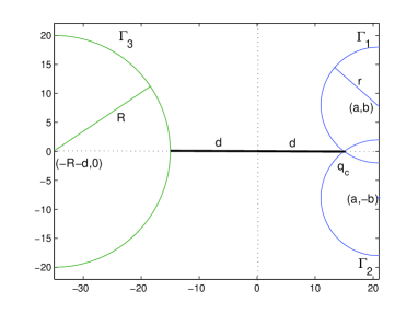
Figure 1: (Color online)The billiard geometry in the 2D case. A cord $\gamma$ is denoted by the bold line.

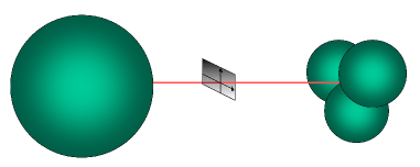
Figure 2: (Color online)The billiard geometry in the 3D case. The cord $\gamma$ is denoted by the solid line.

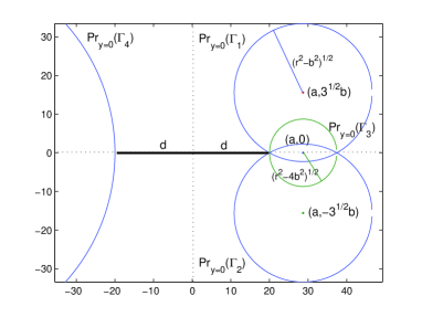
Figure 3: (Color online)The billiard geometry in the 3D case, at the cross section $y=0$. The cord $\gamma$ is denoted by the bold line.

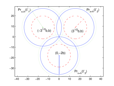
Figure 4: (Color online) The billiard geometry in the 3D case: at the cross-section $x=x_{f}$ the radius of the circles is $r_{f}=\sqrt{r^{2}-(x_{f}-a)^{2}}$. Dotted line: $x_{f}=a$, solid line: $x_{f}=d$, dashed line: $d<x_{f}<a+r$.

Similarly, in the three-dimensional case, we take four spheres (FIG. 2,3,4). Three spheres have equal radii $r$ and have equidistant centers: $(A^{1,2},r^{1,2})=(a,b,\pm\sqrt{3}b,r),$ $(A^{3},r^{3})=(a,-2b,0,r)$. These three spheres intersect, for $r\geq 2b$, at $q_{c}=(d,0,0)$ where $d(a,b,r)=a-\sqrt{r^{2}-4b^{2}}$. The fourth sphere, of radius $R\gg r$, is located at a distance $2d$ from the corner point: $(A^{4},r^{4})=(-R-d(a,b,r),0,0,R)$. The angle between the pairs of tangent lines to the circles of intersections of pairs of spheres is:

$$\alpha_{3D}=\operatorname{acos}(-\frac{1}{2}(1+\frac{3}{(3-r^{2}/b^{2})}))$$ (3)

so $r=2b$ corresponds to the case $\alpha_{3D}=0$. Furthermore, the cord $\gamma=\left\{(x,y,z)|x\in(-d,d),y=z=0\right\}$ is a corner polygon. Here again we can close the billiard domain by adding a finite number of dispersing surfaces which intersect each other in finite angles, or by a large box, so that for all $\alpha>0$ the resulting billiard domain is compact and dispersing. Note that if we rescale all the spheres and the distances between them by a fixed scale $L$, the billiards geometry will not change and the corresponding corner angles remain unchanged.

III Equations of motion for the smooth flow

Consider the smooth motion in this region which is induced by the potential $W(q;w_{0})=\sum_{k=1}^{n}V_{k}(q;w_{0})$; $V_{k}(q;w_{0})$ may be taken as the Gaussian potential associated with the boundary component $\Gamma_{k}$:   $V_{k}(q;w_{0})=V(Q_{k}(q);w_{0})=\exp\left(-\frac{Q_{k}^{2}(q)}{w_{0}^{2}}\right)$, where $Q_{k}(q)$ is the distance between $q$ and the circle $\Gamma_{k}:\quad$$Q_{k}(q)=\sqrt{{\displaystyle\sum\limits_{i=1}^{N}}(q_{i}-A_{i}^{k})^{2}}-r^{k}$ and $w_{0}$ is the softness parameter. In the cold atom experiment $w_{0}$ corresponds to the width of the laser beam kfad01 , and $V(Q_{k}(q);w_{0})$ corresponds to the averaged effective Gaussian potential which bounds the atoms. Previously, we established that as this potential tends to a hard wall potential ($w_{0}\rightarrow 0$), regular reflections of the smooth flow tend to those of the billiard RKTu99 ; RRT05. By the symmetric placement of the spheres, it is clear that for any $w_{0}<w_{0}^{\ast}$ (where $\min_{\gamma}W(q;w_{0}^{\ast})=h$), there exists a periodic solution $\gamma(t,w_{0})=(x(t,w_{0}),0,0)$ which limits, as $w_{0}\rightarrow 0$ to the corner polygon $\gamma$. Notice that studying this system for a fixed $w_{0}$ and a billiard domain which is increased proportionally by a factor $L$ (so $(A^{k},r^{k})\rightarrow(LA^{k},Lr^{k})$), is equivalent to studying it in a fixed geometry with $w_{0}$ replaced by $\epsilon=w_{0}/L$. Thus, by increasing the domain size we may approach the limit $\epsilon\rightarrow 0$ without the numerical problems associated with the stiff limit $w_{0}\rightarrow 0$.

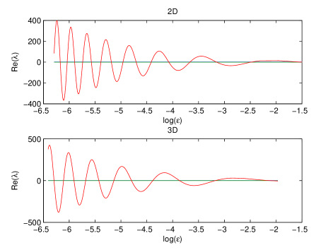
Figure 5: (Color online) The real part of eigenvalue $\lambda$ at $\alpha=0$ as a function of $log(\epsilon)$ for 2D and 3D.

IV Numerical computations

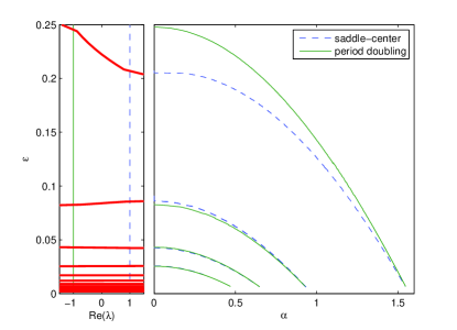
Figure 6: (Color online) 2D. Left: real part of eigenvalue $\lambda$ (bold) at $\alpha=0$. Right: Wedges of stability in the parameter space.

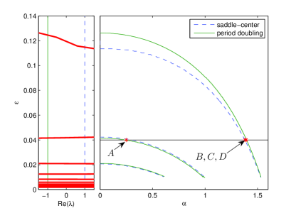
Figure 7: (Color online) 3D. Left: real part of eigenvalue $\lambda$ (bold) at $\alpha=0$. Right: Wedges of stability in the parameter space. See FIG.8 for phase portraits the parameter values corresponding to A-D.

From the analysis of turk03 we expect that the stability of $\gamma(t,\epsilon,\alpha)$ will depend non-trivially on both $\epsilon$ and the geometrical parameter of the billiard $\alpha$ and that near $\alpha_{k}=\frac{\pi}{k}$ islands will appear (the limit $\alpha\rightarrow 0$ at which the billiard is not a Sinai billiard, and thus billiard orbits may be trapped for arbitrarily large number of reflections near the corner has not been studied in turk03 ). We find that all the regions in the $\left(\alpha,\epsilon\right)$ plane at which islands of stability associated with $\gamma(t,\epsilon,\alpha)$ exist (other islands of stability may co-exist), emerge from $\alpha=0$ at some finite $\epsilon_{k}^{\pm}$ values, and converge towards $\left(\alpha,\epsilon\right)\rightarrow(\frac{\pi}{k},0)$. Hence, we first find the stability of $\gamma(t,\epsilon,\alpha=0)$ by computing the eigenvalues of the monodromy matrix of the return map to the local cross-section at $x=0$ for a range of $\epsilon$ values. Since there is always a pair of neutral eigenvalues corresponding to the flow direction, for the 2d case the monodromy matrix has the eigenvalues $\{1,1,\lambda,\frac{1}{\lambda}\}$ where $\lambda$ is the largest eigenvalue which is different from 1. In the 3d case, due to the symmetric form of the geometry, the spectrum is of the form $\{1,1,\lambda,\frac{1}{\lambda},\lambda,\frac{1}{\lambda}\}.$(i.e. saddle-foci do not appear). In FIG. 5 the real part of $\lambda$ is shown for a range of $\epsilon$ values for the 2d and 3d cases. The large oscillations from positive to negative values guarantee the existence of intervals of $\epsilon$ at which  $\operatorname{Re}\{\lambda\}\in(-1,1)$ - on these intervals $\lambda$ is imaginary and belongs to the unit circle. In the left panels of FIG.6 and FIG.7 we present an enlarged segment of FIG. 5 with a regular $\epsilon$ scale. These calculations are used to find the values of $\epsilon=\epsilon_{k}^{\pm}$ at which $\operatorname{Re}\{\lambda\}=\pm 1$, where a saddle-center and a period doubling bifurcations occurs respectively (in the three dimensional case these are double-bifurcation points due to the symmetry). Then, starting at $\left(\alpha,\epsilon\right)=\left(0,\epsilon_{k}^{\pm}\right)$, we use a continuation method for finding the bifurcation curves for $\alpha>0$, as shown in the right panels of FIG.6 and FIG.7. In the wedges enclosed by these two curves the periodic orbit $\gamma(t,\epsilon,\alpha)$ is elliptic, with Flouqet multipliers $\exp(\pm i\omega)$ (in the three dimensional case each multiplier has multiplicity two), and $\omega$ varies between $0$ and $\pi$ as the wedges are crossed. One expects that this linear stability will also result in nonlinear stability for most (non-resonant) $\omega$ values. More elaborate study of the resonances and the relation to the analytic predictions of turk03 are of interest but are beyond the scope of the current paper. For the two dimensional case, we verified that indeed the phase portraits one obtains as a wedge of stability is crossed are the familiar islands which appear near a saddle-center and a Hamiltonian period-doubling bifurcations (e.g. as in the Hamiltonian Hénon map).

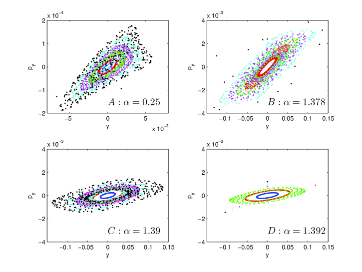
Figure 8: (Color online) 3D. Phase portraits $(y,p_{y})$ at cross-section $x=0,p_{x}>0$ for different values of $\alpha$,$\epsilon=0.04$, see also FIG.7. Notice the different scales for the first stability wedge (B-D) and the second stability wedge (A).

In the three dimensional case, for all $\omega$ values, the multipliers are in $1:1$ resonance due to the symmetry. For generic systems, for almost all $\omega$ values (values which are non-resonant with the frequency of $\gamma(t,\epsilon,\alpha)$), we expect to have non-linear stability (see e.g. MSB86 ). Indeed, projections of the four dimensional symplectic return map to $x=0$ for several $(\alpha,\epsilon)$ values are shown in FIG.8. It is demonstrated that indeed inside the wedged region $\gamma(t,\epsilon,\alpha)$ is nonlinearly stable for the full integration time (approximately 4000 periods). Moreover, if we add a sufficiently small, a-symmetric perturbation to the potential (e.g. $V=W+\delta\cos(y+\eta)\cos(z+\mu)$ with $\delta,\eta,\mu=O(0.0001)$) we find that the effective stability region still persists. For the phase-space simulations we use a symplectic integrator (GniCodes HH03 ), which keeps $h$ up to accuracy of $10^{-11}$. Thus, we can confidently detect islands with transversal kinetic energy of up to $10^{-8}$ (so $(p_{y},p_{z})=O(10^{-4})$). This limits our phase-space calculations to $\varepsilon\approx 0.04$ – smaller values of $\varepsilon$ produce smaller islands and their detection via phase space plots requires a higher accuracy in the integration. We stress though that the calculations of the bifurcation curves are accurate for much smaller $\varepsilon$ values; in these calculation only a single return map is computed and there exists a sharp transition between large positive and large negative values of the eigenvalues (see left panels of FIG. 6,7), so the existence of elliptic regimes is guaranteed. Comparing the 2d and 3d wedges of stability it appears that the 3d wedges are indeed narrower.

V Concluding remarks

While the appearance of islands in two-degrees of freedom steep Hamiltonian systems is somewhat expected, the mechanisms for their appearance in the higher dimensional settings is not as well understood (see MSB86 ; GST04 for some generic possibilities). Furthermore, their appearance guarantees only effective stability due to the possible existence of Arnold diffusion GDFG89 . Nonetheless, by KAM theory, in the non-degenerate case, a large set of initial conditions belongs to KAM tori and thus stay forever near the stable periodic orbit. Thus, the existence of islands in the higher dimensional setting implies that ergodicity is destroyed independently of the possible leakage out of the effective stability zone after an exponentially long time. This latter possibility suggests that stickiness may be an interesting event also in this higher dimensional setting.

Here, we propose for the first time a mechanism for the creation of stability islands for smooth systems which are arbitrarily close to strictly dispersing three dimensional billiards; we showed that potentials $V(q;\epsilon,\alpha)$ that become arbitrarily steep as $\epsilon\rightarrow 0,$ possess wedges in the $(\epsilon,\alpha)$-plane at which a periodic orbit is elliptic. Thus, on one hand, there exist one-parameter families of potentials $V(q;\epsilon,\alpha(\epsilon))$ which have a stable periodic orbit for arbitrarily small $\epsilon$. Since we showed that in the wedges $\alpha(\epsilon)\rightarrow\alpha(0)>0$ as $\epsilon\rightarrow 0$, it follows that these potentials have islands of stability even when they are arbitrarily close to a hard wall dispersing (Sinai) billiards. On the other hand, for any fixed $\alpha\in(0,\frac{\pi}{2})$ there exists an interval of positive $\epsilon$ values for which islands of stability exist. Thus, these islands may be destroyed by either making the potential steeper OR softer – a somewhat non-intuitive result.

VI Acknowledgment

We thank U. Smilansky and D. Turaev for discussions and comments. We acknowledge the support of the Israel Science Foundation (Grant 926/04) and the Minerva foundation.

References

- (1) P. R. Baldwin, Soft billiard systems., Phys. D 29 (1988), no. 3, 321–342.
- (2) P. Bálint and I. P. Tóth, Mixing and its rate in ‘soft’ and ‘hard’ billiards motivated by the Lorentz process, Phys. D 187 (2004), no. 1-4, 128–135, Microscopic chaos and transport in many-particle systems.
- (3) P. Bálint and I.P. Tóth, Hyperbolicity in multi-dimensional Hamiltonian systems with applications to soft billiards, Discrete Contin. Dyn. Syst. 15 (2006), no. 1, 37–59.
- (4) L. A. Bunimovich and J. Rehacek, Nowhere dispersing D billiards with non-vanishing Lyapunov exponents, Comm. Math. Phys. 189 (1997), no. 3, 729–757.
- (5) , How high-dimensional stadia look like, Comm. Math. Phys. 197 (1998), no. 2, 277–301.
- (6) , On the ergodicity of many-dimensional focusing billiards, Ann. Inst. H. Poincaré Phys. Théor. 68 (1998), no. 4, 421–448, Classical and quantum chaos.
- (7) V.J. Donnay, Elliptic islands in generalized Sinai billiards, Ergod. Th. & Dynam. Sys. 16 (1996), 975–1010.
- (8) V.J. Donnay and C. Liverani, Potentials on the two-torus for which the Hamiltonian flow is ergodic., Commun. Math. Phys. 135 (1991), 267–302.
- (9) R. Fleischmann, T. Geisel, and R. Ketzmerick, Magnetoresistance due to chaos and nonlinear resonances in lateral surface superlattices, Physical Review Letters 68 (1992), 1367–1370.
- (10) G. Gallavotti and D.S. Ornstein, Billiards and Bernoulli schemes, Comm. Math. Phys. 38 (1974), 83–101.
- (11) A. Giorgilli, A. Delshams, E. Fontich, L. Galgani, and C. Simó, Effective stability for Hamiltonian systems near an elliptic point, with an application to the restricted three body problem, J. Diff. Eq. 77 (1989), no. 1, 167.
- (12) S. V. Gonchenko, L. P. Shilnikov, and D. V. Turaev, Infinitely many elliptic periodic orbits in four dimensional symplectic diffeomorphism with a homoclinic tangency, Proc. Steklov Inst. Math. 244 (2004), 106–131.
- (13) M.C. Gutzwiller, Chaos in classical and quantum mechanic, Springer-Verlag, New York, NY, 1990.
- (14) E.t Hairer and M. Hairer, GniCodes—Matlab programs for geometric numerical integration, Frontiers in numerical analysis (Durham, 2002), Universitext, Springer, Berlin, 2003, pp. 199–240.
- (15) A. Kaplan, N. Friedman, M. Andersen, and N. Davidson, Observation of islands of stability in soft wall atom-optics billiards, PHYSICAL REVIEW LET 87 (2001), no. 27, 274101–1–4.
- (16) A. Krámli, N. Simányi, and D. Szász, The -property of four billiard balls, Comm. Math. Phys. 144 (1992), no. 1, 107–148.
- (17) I. Kubo, Perturbed billiard systems i the ergodicity of the motion of a particle in a compound central field, Nagoya Math. J. 61 (1976), 1–57.
- (18) J.M. Mao, I.I. Satija, and B. Hu, Period doubling in four-dimensional symplectic maps, Phys. Rev. A (3) 34 (1986), no. 5, 4325–4332.
- (19) J. E. Marsden, Generalized Hamiltonian mechanics: A mathematical exposition of non-smooth dynamical systems and classical Hamiltonian mechanics, Arch. Rational Mech. Anal. 28 (1967/1968), 323–361. MR MR0224935 (37 #534)
- (20) H. Primack and U. Smilansky, The quantum three-dimensional Sinai billiard—a semiclassical analysis, Phys. Rep. 327 (2000), no. 1-2, 107.
- (21) A. Rapoport, V. Rom-Kedar, and D Turaev, Approximating multi-dimensional Hamiltonian flows by billiards, preprint (2006).
- (22) V. Rom-Kedar and D. Turaev, Big islands in dispersing billiard-like potentials, Physica D 130 (1999), 187–210.
- (23) N. Simányi and D. Szász, Hard ball systems are completely hyperbolic, Ann. of Math. (2) 149 (1999), no. 1, 35–96.
- (24) Nándor Simányi, Proof of the ergodic hypothesis for typical hard ball systems, Ann. Henri Poincaré 5 (2004), no. 2, 203–233.
- (25) Ya.G. Sinai, On the foundations of the ergodic hypothesis for dynamical system of statistical mechanics, Dokl. Akad. Nauk. SSSR 153 (1963), 1261–1264.
- (26) , Dynamical systems with elastic reflections: Ergodic properties of scattering billiards, Russian Math. Sur. 25 (1970), no. 1, 137–189.
- (27) Ya.G. Sinai and N.I. Chernov, Ergodic properties of some systems of two-dimensional disks and three-dimensional balls, Uspekhi Mat. Nauk 42 (1987), no. 3(255), 153–174, 256, In Russian.
- (28) U. Smilansky, Semiclassical quantization of chaotic billiards - a scattering approach, Proceedings of the 1994 Les-Houches summer school on ”Mesoscopic quantum Physics” (A. Akkermans, G. Montambaux, and J.L. Pichard, eds.), 1995.
- (29) D. Turaev and V. Rom-Kedar, Soft billiards with corners, J. Stat. Phys. 112 (2003), no. 3–4, 765–813.
- (30) M. Wojtkowski, Linearly stable orbits in -dimensional billiards, Comm. Math. Phys. 129 (1990), no. 2, 319–327.
- (31) G. M. Zaslavsky and H. R. Strauss, Billiard in a barrel, Chaos 2 (1992), no. 4, 469–472.