Analytical description of the coherent structures within the hyperbolic generalization of Burgers equation

Abstract

We present new periodic, kink-like and soliton-like travelling wave solutions to the hyperbolic generalization of Burgers equation. To obtain them, we employ the classical and generalized symmetry methods and the ansatz-based approach

1 Introduction

Actually there are no analytical methods enabling to solve an arbitrary initial or boundary value problems for nonlinear PDEs that are not completely integrable. The majority of evolutionary PDEs used to simulate non-linear transport phenomena is not completely integrable. Yet it is of common knowledge that under certain conditions coherent structures formation take place in open dissipative systems, being simulated by PDEs, that are not completely integrable. The analytical description of the coherent structures within the non-integrable models is of great interest, since analytical form of solution is more preferable in analyzing structures formation and evolution and, besides, they are widely used as a starting point for various asymptotic methods, for testing the numerical schemes and facilitating the stability analysis.

To obtain exact solutions to non-linear PDEs, various methods are used. Besides the classical symmetry reduction scheme (see e.g. [1, 2]), which is not effective in obtaining solutions with the given properties, there are employed techniques based on choosing a proper transformation (or ansatz), turning the problem of finding out exact solutions to the algebraic one [3, 4, 5]. In our previous study [6] we employed a certain dialect of the the direct algebraic method to the hyperbolic generalization of Burgers equation (GBE). Yet in the following publications [7, 8] we showed that within this methodology it is impossible to obtain the the solitary wave solution of GBE, occurring to exist for certain values of the parameters [7]. This served us as a motivation for the developing the effective methods of approximations [7, 8] of solutions describing the coherent structures. Actually we return to the subject of the analytical description of the coherent structures within the GBE model, using for this purpose quite different technique, namely, a generalized symmetry and the combination of the classical symmetry reduction with an ansatz-based method [9].

The structure of the study is following. In section 2 we show how it is possible, combining the classical reduction with the Hirota-like ansatz, to linearize equation describing a set of travelling wave solution to GBE and obtain on this basis new periodic, kink-like and soliton-like solution. In the following section we show how it is possible to gain the linearization of the reduced GBE, using the Painlevé test. In section 4, using the idea of conditional symmetry, we obtain a wide class of exact solutions to GBE, containing the functional arbitrariness. In section 5 we give some examples of such solutions. In the final part of the study we make some conclusions and general remarks.

2 Solutions to GBE obtained via the classical symmetry reduction and Hirota-like ansatz

Let us consider a hyperbolic generalization of Burgers equation [10, 6]:

$$\tau u_{tt}+Auu_{x}+Bu_{t}+H\,u_{x}-\kappa u_{xx}=f(u)=\lambda\,(u-m_{1})(u-m_{2})(u-m_{3}).$$ (1)

We are going to look for the wave patterns among the set of travelling wave (TW) solutions, i.e. solutions invariant with respect to translations generators $\frac{\partial}{\partial\,t}$ and $\frac{\partial}{\partial\,x}$. So it is quite natural to employ the classical reduction scheme [1, 2], and consider an over-determined system containing action of the generator $\hat{X}=\frac{\partial}{\partial\,t}\,-\,\mu\,\frac{\partial}{\partial\,x}$ on the solutions of GBE:

$$\tau u_{tt}+Auu_{x}+Bu_{t}+H\,u_{x}-\kappa u_{xx}=f(u),$$ (2)

$$\hat{X}\,\left[u(t,\,x)-u\right]=u_{t}-\mu\,u_{x}={0}.$$ (3)

The classical theorems [1, 2] assure that system (2)–(3) is compatible and has non-trivial solutions. In fact, solving equation (3) we obtain an ansatz

$$u(t,\,x)=U(\xi),\qquad\xi=x+\mu\,t.$$ (4)

Inserting ansatz (4) into (2), we obtain the following ODE:

$$(\tau\,\mu^{2}-\kappa)\,U^{{}^{\prime\prime}}(\xi)+(H+B\,\mu)\,U^{\prime}(\xi)+A\,U(\xi)\,U^{\prime}(\xi)=\lambda\,(U(\xi)-m_{1})(U(\xi)-m_{2})(U(\xi)-m_{3}).$$ (5)

The problem is that, generally speaking, equation (5) is non-integrable, so, employing the classical reduction scheme we are not able to obtain analytical description to wave patterns.

In the following we use this scheme together with the Hirota-like ansatz

$$U(\xi)=\frac{\Psi^{\prime}(\xi)}{\Psi(\xi)},$$ (6)

and show that under certain conditions such combination leads to a linear ODE. Inserting (6) into (5), we obtain the equation

$$\begin{array}[]{ll}\Psi(\xi)^{2}\bigl{[}\lambda\,m_{1}m_{2}m_{3}\Psi(\xi)-\lambda\,(m_{2}m_{3}+m_{1}m_{2}+m_{1}m_{3})\Psi^{\prime}(\xi)+(H+B\mu)\Psi^{\prime\prime}(\xi)+\\ \\ (\mu^{2}\tau-\kappa)\Psi^{\prime\prime\prime}(\xi)\bigr{]}+\Psi(\xi)\,\Psi^{\prime}(\xi)\bigl{[}\Psi^{\prime\prime}(\xi)\left(A+3\kappa-3\mu^{2}\tau\right)-\Psi^{\prime}(\xi)\left(H-\right.\\ \\ \left.-\lambda\,(m_{1}+m_{2}+m_{3})+B\mu\right)\bigr{]}+\left[\Psi^{\prime}(\xi)\right]^{3}\left(A-\lambda\,-2\kappa+2\mu^{2}\tau\right)=0.\end{array}$$ (7)

One easily gets convinced by the direct inspection that the following statement holds:

Lemma 1

Ansatz (6) leads to the linear ODE

$$\lambda\,\left[m_{1}m_{2}m_{3}\Psi-(m_{2}m_{3}+m_{1}m_{2}+m_{1}m_{3})\Psi^{\prime}\right]+(H+B\mu)\Psi^{\prime\prime}+(\mu^{2}\tau-\kappa)\Psi^{\prime\prime\prime}=0,\quad$$ (8)

provided that following conditions are fulfilled:

$$A+3\kappa-3\mu^{2}\tau=0,$$ (9)

$$H-\lambda\,(m_{1}+m_{2}+m_{3})+B\mu=0,$$ (10)

$$A-\lambda-2\kappa+2\mu^{2}\tau=0.$$ (11)

Equation (8) is a third-order ordinary linear differential equation. Its solutions depend on the roots $\left\{\sigma_{k}\right\}_{k=1,\,2,\,3}$ of corresponding characteristic equation. In case when the conditions (9)–(11), are fulfilled, the characteristic equation is as follows:

$$\sigma^{3}-\left({m_{1}+m_{2}+m_{3}}\right)\,\sigma^{2}+\left(m_{2}\,m_{3}+m_{1}\,m_{2}+m_{1}\,m_{3}\right)\,\sigma-m_{1}\,m_{2}\,m_{3}=0.$$ (12)

The roots of equation (12) coincide with the numbers $m_{1}$, $m_{2}$ and $m_{3}$, being the roots of equation $f(u)=0$. Below we consider four distinct cases.

Case I. For $m_{1}\neq m_{2}\neq m_{3}\neq m_{1}$ the general solution of (8) takes on the form

$$\Psi(\xi)=e^{m_{1}\,\xi}c_{1}+e^{m_{2}\,\xi}c_{2}+e^{m_{3}\,\xi}c_{3}.$$

In the following we put $c_{1}=1$. With this assumption we obtain the expression

$$u(t,\,x)=\frac{m_{1}e^{m_{1}\xi}+c_{2}m_{2}e^{m_{2}\xi}+c_{3}m_{3}e^{m_{3}\xi}}{e^{m_{1}\xi}+c_{2}e^{m_{2}\xi}+c_{3}e^{m_{3}\xi}},\quad\xi=x+\mu t.$$ (13)

For positive $c_{2}\,\,\mbox{and}\,\,c_{3}$ formula (13) describes a kink-like solution (see fig 1).

Figure 1: An example of TW solution described by the formula (13)

Case II: For $m_{1}\neq m_{2}=m_{3}$

$$\Psi(\xi)=e^{m_{1}\xi}+e^{m_{2}\xi}(c_{2}+c_{3}\xi)$$

and using the formula (6) we get the solution

$$u(t,\,x)=\frac{m_{1}e^{m_{1}\xi}+c_{3}e^{m_{2}\xi}(c_{2}\,m_{2}+c_{3}+m_{2}\,c_{3}\xi)}{e^{m_{1}\xi}+e^{m_{2}\xi}(c_{2}+c_{3}\xi)}.$$ (14)

Asymptotic analysis shows, that solution (14) tends to either $m_{1}$ or to $m_{2}$ as $\xi\rightarrow\pm\,\infty$. The condition of non-singularity of the solution reads as follows: $\forall\xi\in R:$ $e^{m_{1}\xi}+e^{m_{2}\xi}(c_{2}+c_{3}\xi)>0$ or, in other words,

$$e^{(m_{1}-m_{2})\xi}>-(c_{2}+c_{3}\xi).$$ (15)

It is possible when $m_{1}-m_{2}$ is positive, and $c_{3}$ is negative or when $m_{2}-m_{1}$, and $c_{3}$ are positive. In fig. 2 the first possibility is illustrated. Note that the second one is symmetric. It is evident from the analysis of fig. 2 that condition (15) is satisfied in case when $-c_{2}<c_{cr}$. One can easily verify that $c_{cr}$ is expressed by the formula

$$\qquad c_{cr}=-A\left[c_{3}+e^{m_{1}-m_{2}}\right],$$

providing that $A=\frac{1}{m_{1}-m_{2}}\,ln\,\frac{c_{3}}{m_{2}-m_{1}}.$

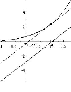
Figure 2: Case II: nonsingular solutions. Solid lines correspond to the plots of functions $f_{1}(\xi)=e^{(m_{1}-m_{2})\xi}$ and $f_{2}(\xi)=-(c_{2}+c_{3}\xi)$. Dashed line is a tangent to $f_{1}(\xi),$ being parallel to $f_{2}(\xi)$

Figure 3: An example of TW solution described by the formula (14)

Case III: For $m_{1}=m_{2}=m_{3}=m$

$$\Psi(\xi)=e^{m\xi}\,\left[c_{3}+\xi\,(c_{2}+\xi)\right]$$

and using (6) we get the solution

$$u(t,\,x)=m+\frac{c_{2}+2\xi}{c_{3}+\xi(c_{2}+\xi)},$$ (16)

Formula (16) describes a a solitary wave with ”heavy” tails (fig. 4), providing that inequality $c_{2}^{2}-4\,c_{3}<0$ holds.

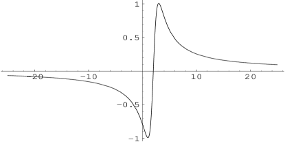
Figure 4: An example of TW solution described by the formula (16)

Case IV: For $m_{1},\,\,m_{2}=\alpha\pm\,\beta\,i$, and real $m_{3},$ we get the solution

$$u(\xi)=\frac{c_{3}m_{3}e^{m_{3}\xi}+2e^{\alpha\xi}\left[\alpha\,\mbox{cos}(\beta\xi)-\beta\,\mbox{sin}(\beta\xi)\right]}{c_{3}e^{m_{3}\xi}+2\,e^{\alpha\xi}\mbox{cos}(\beta\xi)}$$ (17)

Let us notice, that the only possibility for the solution (17) to be non-singular is simultaneous fulfillment of the conditions $m_{3}=\alpha$ and $|c_{3}|>2.$ In this case we get a periodic solution (fig. 5).

3 Painlevé analysis of GBE

Now we are going to show how the conditions on constants similar to (9)–(11) can be obtained using the Painlevé test [11]. Since we concentrate here merely upon the set of TW solutions, let’s start from the equation (5).

In the first step we take $U(\xi)=U(x+\mu t)=a[0]\xi^{p}$ and put it into the leading terms of (5). This way we obtain the relation:

$$(p-p^{2})(\mu^{2}\tau-\kappa)+A\,p\,\xi^{p+1}a[0]+\lambda\,\xi^{2p+2}a[0]^{2}=0.$$ (18)

In order that the equation be balanced, we must put $2(p+1)=p+1$, so $p=-1$.

Next we take $U(\xi)=\sum_{i=0}^{\infty}a[i]\xi^{i-1}$. Equating to zero coefficients of each power of $\xi$, we get the recurrence for $a[i]$. The first two expressions are as follows:

$${\kappa\lambda}\,a[0]={A\pm\sqrt{A^{2}-8\lambda\,(\mu^{2}\tau-\kappa)}}$$ (19)

$$(A-3\lambda\,a[0])a[1]=-(H+B\mu+\lambda\,(m_{1}+m_{2}+m_{3})a[0])$$ (20)

Since in the Painlevé test being applied to a second order equation one of $a[i]$ should be ”free”, then we can put

$$\begin{array}[]{ll}A-3\lambda\,a[0]=0\\ H+B\mu+\lambda\,(m_{1}+m_{2}+m_{3})a[0]=0.\\ \end{array}$$ (21)

Solving (21) we obtain:

$$\lambda\,=\frac{s^{2}}{\mu^{2}\tau-\kappa},\qquad A=-3s,\qquad s=\frac{H+B\mu}{m_{1}+m_{2}+m_{3}}.$$

If we additionally put $a[0]=1$ then we get precisely the conditions for which equation (7) linearizes.

Figure 5: Periodic TW solution to (2) described by the formula (17)

4 Exact solutions of GBE associated with the conditional symmetry

Now let us consider an over-determined system

$$\tau u_{tt}-\kappa u_{xx}+u\,u_{x}+u_{t}=f(u),$$ (22)

$$\hat{X}\,[u]=\nu\,u_{t}+u_{x}\,=\,\Phi(u),$$ (23)

where

$$\hat{X}=\nu\partial_{t}+\partial_{x}+\Phi(u)\partial_{u}$$ (24)

is a generalized (conditional) symmetry generator containing an unknown function $\Phi(u)$.

In accordance with [12, 13, 14], system (22–23) will be compatible if it admits the second prolongation of the operator $\hat{X}$:

$$\hat{X}_{2}=\hat{X}+\zeta_{xx}\,\frac{\partial}{\partial u_{xx}}\,+\zeta_{t}\,\frac{\partial}{\partial u_{t}}+\zeta_{x}\,\frac{\partial}{\partial u_{x}}+\zeta_{tt}\,\frac{\partial}{\partial u_{tt}}+\zeta_{tx}\,\frac{\partial}{\partial u_{tx}}$$ (25)

where

$$\zeta_{t}=D_{t}\,\Phi(u),\quad\zeta_{x}=D_{x}\,\Phi(u),\quad\zeta_{tt}=D_{t}\,\zeta_{t},\quad\zeta_{tx}=D_{t}\,\zeta_{x},\quad\zeta_{xx}=D_{x}\,\zeta_{x}$$

and $D_{t},\,D_{x}$ are total derivatives with respect to corresponding variables. Applying the operator (25) to equation (22), we get:

$$\zeta_{t}+\tau\,\zeta_{tt}+\Phi(u)\,u_{x}+u\,\zeta_{x}-\kappa\,\zeta_{xx}-\dot{f}(u)\,\Phi(u)|_{E_{i}=0}=0,$$ (26)

where $E_{i}=0$ means that equation is considered on the manifold, i.e. when equations (22)–(23) and all their differential consequences are taken into account.

A passage to the manifold defined by equations (22)–(23) requires some comments. Equation (23) and its differential consequences give us the following conditions:

$$u_{x}=\Phi(u)-\nu\,u_{t},$$ (27)

$$u_{xx}=\dot{\Phi}(u)\,\Phi(u)-2\,\nu\,\dot{\Phi}(u)\,\,u_{t}+\nu^{2}\,u_{tt}.$$ (28)

Using these formulae and equation (22), we can also exclude $u_{tt}$. In fact, inserting (27)–(28) into (22), we obtain the equation

$$\left(\tau-\kappa\,\nu^{2}\right)\,u_{tt}=f(u)+\left(\nu\,u-1-2\,\kappa\,\nu\,\dot{\Phi}(u)\right)\,u_{t}+\Phi(u)\left(\kappa\,\dot{\Phi}(u)-u\right).$$ (29)

Here we have two possibilities, depending on whether $\left(\tau-\kappa\,\nu^{2}\right)$ is zero or not.

If $\tau-\kappa\,\nu^{2}\,\neq\,0,$ then, returning to (26) and taking account of (27)–(28) and (29), we obtain a first order PDE. Applying the standard procedure of splitting [12, 13, 14] and solving the system of determining equations we conclude that $\Phi[u]=0$ and therefore $\hat{X}$ is a classical symmetry generator.

Now let us assume that $\tau-\kappa\,\nu^{2}\,=\,0.$ Using the formulae (27)–(28), we can exclude from (26) merely the spatial derivatives $u_{x}$ and $u_{xx}$. The splitting procedure gives us in this case the following system:

$$\kappa\,\left\{{\Phi}(u)\ddot{\Phi}(u)+\left[\dot{\Phi}(u)\right]^{2}\right\}={\Phi}(u)+u\,\dot{\Phi}(u)-\dot{f}(u)$$ (30)

$$2\,\kappa\,\nu\,\left\{{\Phi}(u)\ddot{\Phi}(u)+\left[\dot{\Phi}(u)\right]^{2}\right\}=\left(\nu\,u-1\right)\dot{\Phi}(u)+\nu\,{\Phi}(u)$$ (31)

Integrating once equations (30)–(31), we get the system

$$\kappa\,\Phi(u)\dot{\Phi}(u)=u\,{\Phi}(u)-{f}(u)-C_{1},$$ (32)

$$2\,\kappa\,\nu\,{\Phi}(u)\dot{\Phi}(u)=\left(\nu\,u-1\right)\,{\Phi}(u)+C_{2}.$$ (33)

Multiplying (32) by $2\,\nu$ and extracting the resulting equation from (33), we get the relation between the functions $\Phi(u)$ and $f(u)$:

$$\Phi\,(u)=\frac{2\,\nu\,\left[f(u)+C_{1}\right]+C_{2}}{\nu\,u+1}\,.$$ (34)

Let us note that function $\Phi\,(u)$ is defined by the Abel-type equation (33). Passing to the new independent variable $\zeta=\left(\nu\,u-1\right)\,C_{2}/\left(2\,\kappa\,\nu^{2}\right),$ we can bring it to the canonical form [15]:

$${\Phi}(\zeta)\frac{d\,\Phi(\zeta)}{d\,\zeta}=\alpha\,\zeta\,{\Phi}(\zeta)+1,\qquad\alpha=\frac{2\,\kappa\,\nu^{2}}{C_{2}^{2}}.$$

A passage to the new variables

$$\xi=\Phi-\frac{\alpha}{2}\,\Psi^{2}\left(\xi\right)$$

leads to the Riccati equation

$$\frac{d\,\Psi}{d\,\xi}=\frac{\alpha}{2}\,\Psi^{2}+\xi.$$

Solution to this equation is expressed by the following formula [15]:

$$\Psi\left(\xi\right)=\sqrt{\xi}\left[A\,J_{\frac{1}{2q}}\left(\frac{1}{q}\sqrt{\frac{\alpha}{2}}\,\xi^{q}\,\,\right)+B\,Y_{\frac{1}{2q}}\left(\frac{1}{q}\sqrt{\frac{\alpha}{2}}\,\xi^{q}\,\right)\right],\qquad q=\frac{3}{2},$$ (35)

where $A,\,\,B$ are constant parameters while $J_{m}(z),\,\,Y_{m}(z)$ are the Bessel functions.

So, in accordance with the formulae (35) and (34), $f(u)$ is expressed in a complicated way by special functions. In order to obtain an explicit description to $f(u)$, we set $C_{1}=C_{2}=0$. In this case system (32)–(33) has the following solution:

$$f(u)=h_{0}+\left(\nu\,h_{0}-\frac{1}{4\,\kappa\,\nu^{2}}\right)\,u-\frac{1}{8\,\kappa\,\nu}\,u^{2}+\frac{1}{8\,\kappa}\,u^{3},$$ (36)

$$\Phi(u)=\frac{\nu\,u^{2}-2\,u+8\,\nu^{2}\,h_{0}\,\kappa}{4\,\nu\,\kappa},$$ (37)

where $h_{0}$ is an arbitrary constant. Now we are going to formulate the main result of this section.

Theorem 1

Suppose that $f(u)$ and $\Phi(u)$ are given by the formulae (36) and (37) respectively. Then

• system (22)-(23) is compatible;

• every solution of (23) satisfies (22).

5 Examples of conditionally-invariant solutions of GBE

For $\nu=\tau=\kappa=1$ equation (23) takes the form

$$u_{t}+u_{x}=\frac{1}{4}\,\left(u^{2}-2\,u+8\,h_{0}\right).$$ (38)

General solution of this equation depends on whether $\Delta=1-8\,h_{0}$ is positive or not. For $h_{0}<1/8$ solution of (38) is as follows:

$$u(t,\,x)=\frac{u_{2}\,G(\omega)\,e^{t\,\frac{\sqrt{\Delta}}{2}}-u_{1}}{G(\omega)\,e^{t\,\frac{\sqrt{\Delta}}{2}}-1}\,,$$ (39)

where

$$u_{1}=1+\sqrt{\Delta}\,,\qquad u_{2}=1-\sqrt{\Delta}\,,$$

$G(\cdot)$ is an arbitrary function of $\omega=x-t$. Putting $h_{0}=-1$ and $G(\omega)=-e^{\Gamma(\omega)}$ we obtain the formula

$$u(t,\,x)=2\,\frac{2-\mbox{exp}[3\,t/2+\Gamma(\omega)]}{1+\mbox{exp}[3\,t/2+\Gamma(\omega)]}.$$ (40)

For $h_{0}=-1$ and $G(\omega)=e^{\Gamma(\omega)}$ we get the solution

$$u(t,\,x)=2\,\frac{\mbox{exp}[3\,t/2+\Gamma(\omega)]+2}{1-\mbox{exp}[3\,t/2+\Gamma(\omega)]}.$$ (41)

If $h_{0}>1/8$ then solution to (38) is as follows:

$$u(t,\,x)=1+\beta\,\mbox{arctg}\left[\frac{\beta\,t}{4}+G(\omega)\right],$$ (42)

where $\beta=\sqrt{|1-8\,h_{0}|}$. This solution is always singular.

If $h_{0}=1/8$ then solution to (38) is as follows:

$$u(t,\,x)=1+\frac{1}{G(\omega)-\frac{t}{4}},$$ (43)

This solution is also singular.

Let us give examples of solutions corresponding to formulae (40) and (41). Thus, inserting $\quad\Gamma(\omega)=\mbox{sin}\,[2.25\,\omega]$ into equation (41), we obtain an oscillating kink-like solution, shown in fig. 6. For $\Gamma(\omega)=-\omega^{2}$ this solution produces a ”dark” soliton with a growing support (fig 7).

In contrast to (40), solution (41) is always singular. For $\Gamma(\omega)=-3.75\,\omega^{2}+5$ its evolution is shown in fig. 8, in which we see how an initial localized wave pack grows in amplitude and in a finite time gives rise to a blow-up regime.

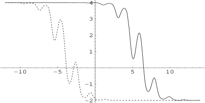
Figure 6: Temporal evolution of solution described by formula (40) in case when $\Gamma({\omega})=\mbox{sin}[2.25\,\omega]$

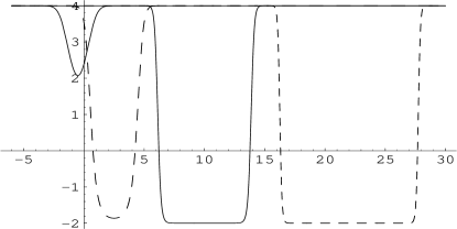
Figure 7: Temporal evolution of solution described by formula (40) in case when $\Gamma(\omega)=-\omega^{2}$

Figure 8: A blow-up regime described by the formula (41) in case when $\Gamma(\omega)=-3.75\,\omega^{2}+5$

6 Concluding remarks

In this study new solutions to GBE, describing wave patterns formation and evolution have been obtained by means of classical and generalized symmetry methods and ansatz-based approach. Most of these solutions cannot be obtained within the dialects of direct algebraic methods, previously applied to this equation [6].

Let us discuss the solutions obtained in section 2. In the case when $m_{1}\neq m_{2}\neq m_{3}\neq m_{1}$ we deal with solutions described by a rational combination of the exponential functions which, generally speaking, do not coincide with the powers of a single exponential function as it was the case in [6]. In the following cases considered in section 2, solutions are described as rational combinations of exponential, polynomial and trigonometric functions and such combinations were never applied to GBE before.

Solutions obtained in section 4 contain arbitrary functions, depending on the linear combination of spatio–temporal variables. From one hand, it allows, by a proper choice of these functions, to construct a variety of different solutions, such as those presented in section 5. From the other hand, appearance of an arbitrary function can be employed to describe a sufficiently wide family of an initial and (or) boundary value problems. Obtaining of such solutions has become possible due to employment of conditional symmetry.

The results presented in section 2 suggest that the possibilities of obtaining new solutions for GBE within the ansatz-based methods are not exhausted. It should be noted, however, that effectiveness of these methods grows in the situation when they are combined with another methods such as symmetry reduction or the Painlevé test. As it was shown in section 4, application of the methods based on conditional symmetry is also very promising. Let us note in conclusion, that for GBE the most simple conditional symmetry has been obtained as yet. Our preliminary investigations show, that there are another conditional symmetry operators admitted by GBE, which seem to be very promising from the point of view of obtaining new sets of solutions.

References

[1]
L.V. Ovsiannikov, Group Analysis of Differential Equations, New
York, Academic Press, 1982.
[2]
P. Olver, Applications of Lie groups to differential equations,
New York, Springer, 1993.
[3]
E. Fan, Journ of Physics A: Math and Gen, 35, (2002),
6853–6872.
[4]
A. Nikitin, T. Barannyk, Solitary Waves and Other Solutions
for Nonlinear Heat Equations, arXiv:math-ph/0303004 (2003).
[5]
A. Barannyk, I. Yurik, Proceedings of Institute of
Mathematics of NAS of Ukraine, 50, Part I (2004), 29–33.
[8]
V.A. Vladimirov, E.V. Kutafina and A. Pudełko, SIGMA, 2 (2006), Paper 016, 15 p.
[9]
P. Clarkson and L. Mansfield, Physica D, 70 (1993),
250–288.
[10]
A. Makarenko, Control and Cybernetics, 25 (1996),
621–630.
[11]
M. Tabor, Chaos and Integrability in Nonlinear Dynamics: An
Introduction, New York, Wiley, 1989.
[12]
W. Fushchych, W. Shtelen, N. Serov, Symmetry Analysis and Exact
Solutions of Equations of Nonlinear Mathematical Physics,
Dordrecht, Kluver Publishers, 1993.
[13]
P. Olver and P. Rosenau, Phys. Lett., A 114 (1986),
107–112.
[14]
P. Olver, E. Vorob’jev, Nonclassical and conditional symmetries,
in: CRC Handbook of Lie Group Analysis of Differential Equations,
Volume III, ed. by Nail Ibragimov. - CRC Press Inc, 2000.
[15]
V.F. Zajtsev and A.D. Polyanin, A reference Book of the Ordinary
Differential Equations, Moscow, Fiz.-Mat. Lit. Publ., 2001 (in
Russian).