Excitability in a nonlinear magnetoacoustic resonator

Abstract

We report a nonlinear acoustic system displaying excitability. The considered system is a magnetostrictive material where acoustic waves are parametrically generated. For a set of parameters, the system presents homoclinic and heteroclinic dynamics, whose boundaries define a excitability domain. The excitable behaviour is characterized by analyzing the response of the system to different external stimuli. Single spiking and bursting regimes have been identified.

There is an increasing interest in the study of smart materials smart . The term smart refers to a class of materials that are highly responsive and have the inherent capability to sense and react according to changes in the environment. The most widely used classes of smart materials are ferroic, and include piezoelectrics, electrostrictors, magnetostrictors, and shape-memory alloys. In this letter we consider a smart system based on the magnetostrictive effect. Magnetostriction is the material property that causes a material to change its dimensions under the action of a magnetic field or, inversely, to generate a magnetic field when deformed by an external force. Magnetostrictive materials can thus be used for both sensing and actuation.

One of the main goals of smart materials research is to design systems able to mimic biological behaviour. For example, artificial muscles have been recently developed based on electroactive polymers. Possibly the smartest biological system is the neuron, responsible among others of the signal processing in the brain. This processing capability relies to a large extend on a property on the individual neurons called excitability Izhikevich00 . The most characteristic feature of excitability is a highly nonlinear response (of all–or–nothing type) to an external stimulus: when the amplitude of the stimulus is below a given threshold, there is a weak reaction, while the response is strong, but independent of the strength of the stimulation, above the threshold. The interest in excitable systems came first from chemistry (reaction–diffusion systems) and biology (cardiac tissue and neural modeling) Murray90 . More recently, excitability has been identified in certain optical systems, as the CO₂ laser with saturable absorber Plaza97 or the semiconductor laser with optical feedback Giacomelli00 . In this letter we report on the first, to the best of our knowledge, acoustic system displaying excitability. The system also displays a rich complex behaviour including an scenario of homoclinic/heteroclinic dynamics, which is on the basis of the excitable character of the system.

The considered physical system consists in a magnetostrictive material (e.g., a ferrite) in the form of a rod with transverse section $S$ and length $L,$ with parallel and flat lateral boundaries, which is driven by an external magnetic field $H_{ext}=H_{0}+H_{q}(t)$ parallel to the axis of the rod. The oscillating magnetic field $H_{q}(t)=h\cos(2\omega t)$ induce a temporal modulation of the sound velocity in the material at frequency $2\omega$, which is responsible for the parametric excitation of an acoustic wave in the material at half of the driving frequency. A standing wave is formed since the polished boundaries define a high-Q resonator for the sonic beam. This effect has been considered in a number of works Brysev98 ; Brysev00 ; Preobrazhensky93 , where a radiofrequency magnetic field was used to excite parametrically an ultrasonic wave. In these works, a special attention was paid to the phenomenon of phase conjugation (PC) of an incident acoustic beam, with important applications in e.g. acoustic microscopy Brysev002 .

In the simplest scheme, the oscillating magnetic field is produced by a coil with $n$ turns surrounding the material, The coil provides the inductance of an electric RLC series circuit, driven by an ac source at frequency $2\omega$ and variable amplitude $\mathcal{E}$. Owing to magnetoelastic coupling, elastic deformations in the magnetostrictive material result in an additional magnetic field. Following Brysev98 ; Preobrazhensky93 , we consider that the dominant contribution of the magnetoelastic interaction is quadratic in the particle displacements $H_{int}(t)=-\alpha~{}\left\langle u(\mathbf{r},t)^{2}\right\rangle$, where $\alpha=(2k)^{2}(\partial\ln v/\partial H)$ is the coupling coefficient proportional to the modulation depth of sound velocity Preobrazhensky93 , and the brackets indicate a spatial average over the material volume. Taking into account the magnetoelastic contribution, the effective magnetic excitation in the material takes the form $H=H_{ext}(t)+H_{int}(t).$ The resulting magnetic induction $B=\mu\left(H\right)H$ is in general a nonlinear relation, which to the leading order can be written as $B=\mu H+\frac{1}{6}\mu_{0}\chi^{(3)}H^{3}$ Streltsov97 , where $\mu$ is the linear permeability of the material and $\chi^{(3)}$ the third order magnetic susceptibility, which in turn depends on the frequency.

A nonlinear equation for the electric circuit can be obtained under the previous assumptions, and neglecting nonresonant terms and those higher than quadratic in $H_{q}$ and $H_{int}$. It reads

$$\mathcal{L}\frac{d^{2}q}{dt^{2}}+R\frac{dq}{dt}+\frac{q}{C}=\mathcal{E}\cos(2\omega t)+$$

$$\mu n\alpha\frac{d}{dt}\left\langle u^{2}\right\rangle+\mu_{0}\chi^{(3)}n^{2}H_{0}\alpha\frac{d}{dt}\left(\frac{dq}{dt}\left\langle u^{2}\right\rangle\right),$$ (1)

where $q$ is the charge in the capacitor, related with the current as $I=dq/dt$, $\mathcal{L}$ is the coil inductance and $H_{q}=nI.$ The last two terms result from the nonlinearities related to magnetoelastic interaction and magnetic nonlinearity.

The acoustic field obeys the wave equation with a source (coupling) term proportional to the exciting magnetic field Preobrazhensky93 . In terms of the charge it reads

$$\frac{1}{v^{2}}\frac{\partial^{2}u}{\partial t^{2}}-\nabla^{2}u=\alpha n\frac{dq}{dt}u.$$ (2)

We consider solutions of Eqs. (1) and (2) in the form of quasi-harmonic waves, i.e., whose amplitudes are slowly varying in time. In this case we can write

$$q\left(t\right) =\frac{1}{2}\left[Q\left(t\right)\exp\left(2i\omega t\right)+c.c.\right],$$ (3a)

$$u\left(\mathbf{r},t\right) =\frac{1}{2}\left[U\left(t\right)\exp\left(i\omega t\right)+c.c.\right]g\left(\mathbf{r}_{\bot}\right)\sin\left(kz\right),$$ (3b)

where $$u\left(\mathbf{r},t\right) k=m\pi/L 2\omega=1/\sqrt{\mathcal{L}C}$$ is an eigenmode of the acoustical resonator, define the cavity resonances, and is the pumping frequency at the circuit resonance. In the slowly-varying envelope approximation, the amplitudes obey the evolution equations (see Sanchez05 for details)

$$\frac{dX}{d\tau} =\mathcal{P}-X+Y^{2}+i\eta\left|Y\right|^{2}X,$$ (4)

$$\frac{dY}{d\tau} =-\gamma\left(Y-XY^{\ast}\right),$$

where $X$ and $Y$ are normalized values of the charge in the capacitor and the amplitude of the ultrasonic field, respectively, which relate to the physical variables through the transformations $X=\left(v^{2}n\alpha/2\gamma_{U}\right)Q\$and$\ Y=\frac{1}{4}\left(v\alpha n\right)(\mu L/\mathcal{L}\gamma_{U}\gamma_{Q})^{1/2}U.\$The pumping term$\ \mathcal{P}=(v^{2}n\alpha/4\omega\gamma_{U}R)\mathcal{E}$ is proportional to the voltage of the ac source. The parameter $\gamma=\gamma_{U}/\gamma_{Q}$ represents the ratio between losses, being $\gamma_{Q}=R/2\mathcal{L}\$and $\gamma_{U}$ the electric and acoustic decay rates respectively. The last parameter is introduced phenomenologically, and take into account the losses due mainly to radiation from the boundaries. A dimensionless time $\tau=\gamma_{Q}t$ has been also defined. Finally, $\eta=4\omega H_{0}\gamma_{U}\chi^{(3)}/\alpha v^{2}\mu_{r}$ remains as the single parameter of nonlinearity, with $\mu_{r}=\mu/\mu_{0}$. Due to the number of parameters involved in $\eta$, it can be varied over a wide range of values. Note that Eqs. (4) also possess the $\emph{Z}_{2}$ (reflection) symmetry $(X,Y)\rightarrow(X,-Y)$.

The stationary solutions of Eqs. (4) and their stability have been analysed in Sanchez05 . This analysis showed that the trivial solution $X=\mathcal{P},\ Y=0$, where the acoustic subharmonic field is switched-off, experiences a subcritical pitchfork bifurcation at $\mathcal{P}=1$, the parametric generation threshold, and gives rise to a finite amplitude solution $\left|X\right|=1,$ $\left|Y\right|^{2}=(1\pm\sqrt{\mathcal{P}^{2}(1+\eta^{2})-\eta^{2}})/(1+\eta^{2}).$ Subcriticality implies a domain of coexistence between the trivial (rest) state and the finite-amplitude solution when $\mathcal{P}_{T}<$ $\mathcal{P}<1,$ where $\mathcal{P}_{T}=\eta/\sqrt{1+\eta^{2}}$ is the turning point. For some values of the parameters, the finite amplitude solution can experience a Hopf (selfpulsing) instability, whose analytical expression was also given in Sanchez05 . The boundaries of these local instabilities are depicted in Fig.1.

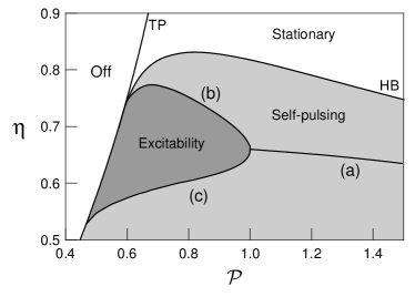
Figure 1: Bifurcation diagram of Eqs. (4) for $\gamma=0.1.$ Local bifurcations are denoted by TP (fold or turning point), HB (Hopf bifurcation), and the line $\mathcal{P}=1$ corresponding to the subcritical pitchfork bifurcation (parametric generation threshold). Three curves labeled as (a), (b) and (c) denote the locus of global bifurcations (see text for details).

In Sanchez05 it was also shown that the system possess homoclinic (global) dynamics at a particular value of the nonlinearity parameter $\eta$. In this letter we perform a detailed two-parameter numerical analysis of Eqs. (4). For this aim, we reduce the dimensionality of the parameter space by fixing the value of the relative losses $\gamma=0.1$, which is in correspondence with typical experimental conditions Brysev00 . The results for other values of $\gamma$ are qualitatively similar.

The bifurcation diagram shown in Fig. 1 reveals that the system presents a complex scenario of global dynamics. Besides the Hopf bifurcation leading to self-pulsing, three different global bifurcations have been identified in this system. These bifurcations can be detected numerically by computing the period of the limit cycles, since close to a homoclinic/heteroclinic point the period diverges to infinity as $T=-\frac{1}{\lambda}\ln(\mathcal{P}_{h}-\mathcal{P})$, where $\mathcal{P}_{h}-\mathcal{P}$ measures the distance to the homoclinic bifurcation (which is assumed small) and $\lambda$ is the eigenvalue in the unstable direction of the saddle point Gaspard90 . In Fig. 1, infinite period ($T_{\infty}$) bifurcations are the curves labeled (a)-(c). Curve (a) corresponds to a gluing (double homoclinic) bifurcation Glendinning84 . This bifurcation is characteristic of systems with $Z_{2}$ symmetry and is mediated by a saddle point, which in this case corresponds to the trivial state. The gluing bifurcation exists for a broad range of pump values, and persists until the pitchfork bifurcation, at $\mathcal{P}=1.$ At this point, two new branches of $T_{\infty}$ bifurcations emerge. The upper branch (b) correspond to a homoclinic bifurcation connecting one saddle with itself, while the lower branch (c) corresponds to a heretoclinic connection between two symmetric saddles. Three phase portraits corresponding to the different global bifurcations are shown in Fig. 2. The simultaneous presence of the three reported types of global bifurcations is a unusual phenomenon. We note that a similar picture results from the analysis of two coupled van der Pol oscillators with delay coupling Wirkus02 , however in a quite different context.

Figure 2: Phase portraits of the acoustic field for parameters close to the different global bifurcations: (a) gluing, for $\eta=0.65$ and $\mathcal{P}=1.22$, (b) homoclinic, for $\eta=0.7$ and $\mathcal{P}=0.96$, and (c) heteroclinic, for $\eta=0.65$ and $\mathcal{P}=1$.

The period of limit cycle solutions, as the pump parameter is varied, is shown in Fig. 3 for two representative values of the nonlinearity parameter $\eta$, below (dashed line) and above (continuous line) the codimension–three point where all the global bifurcations coalesce, at $\eta\approx 0.67$. As expected from Fig. 1, at $\eta=0.7$ there is only one $T_{\infty}$ bifurcation, consisting in a homoclinic loop as shown in Fig. 2(b). For $\eta=0.65,$ both gluing bifurcation [Fig. 2(a)] and heteroclinic connection [Fig. 2(c)] coexist. It is remarkable that this situation has been also described for a periodically forced Navier-Stokes flow in hydrodynamics Lopez00 .

Figure 3: Period of time-dependent solutions depending on the pump, for $\eta=0.65$ (full line) and $\eta=0.7$ (dashed line). The period diverges to infinity at some values, denoting the presence of gluing (a), homoclinic (b) and heteroclinic (c) bifurcations.

One prominent property found in some systems presenting homoclinic dynamics is excitability. As stated above, excitable systems present a highly nonlinear response to an external stimulus, with a well defined excitability threshold and a constancy in the reaction when perturbed above threshold. In addition, a refractory time has to elapse before the system can be excited again. These neuron–like properties can be also present in the magnetoacoustic resonator considered here, as we demonstrate below.

The key for achieving excitability is the coexistence of a global bifurcation and a stable fixed point Izhikevich00 . This occurs in the dark-shadowed region in Fig. 1. The excitability properties of a system can be characterized in several ways, in terms of its respose to different kinds of external perturbations. In order to demonstrate the main signatures described above, we consider first the behaviour of the system under a short (delta-like) perturbation. Figure 4(a) shows the amplitude response of the acoustic field after four perturbations with increasing amplitude, for parameter values $\eta=0.7$, $\mathcal{P}=0.94$ and $\gamma=0.1$ (close to the homoclinic bifurcation boundary, curve (b) in Fig.1). The system, initially at rest, is perturbed at $t=0.$ The amplitude of the weakest perturbation was chosen to be below the excitability threshold $y_{th}$ (determined by the distance from the node to the saddle point), and the system relaxes smoothly to the rest. Three perturbations above the threshold, with different amplitudes, however generate three identical pulses or spikes. The amplitude of the perturbation only affects to the response time of the system: when stronger the stimulus, the smaller the time needed to develope a pulse.

Figure 4: Amplitude of the acoustic field in response to four external perturbations of increasing amplitude, for $\eta=0.7$ and $\mathcal{P}=0.94$ (a). Delay time (dots) as a function of the strength of the perturbation. The inset corresponds to a logaritmic representation of the numerical data, and the continuous line to Eq. (6).

The delay time has been measured as the interval between the stimulus and the instant where the pulse reaches the maximum amplitude, for different overthreshold perturbations. The results are shown in Fig. 4(b). The inset corresponds to the logarithmic representation of the numerical data, and demonstrates that the scaling law for the response time is ruled by the same law as the period of limit cycles close to homoclinic/heteroclinic bifurcations, i.e.

$$\tau_{delay}=-\frac{1}{\lambda}\ln(y-y_{th})+c,$$ (5)

where $\lambda$ again corresponds to the unstable eigenvalue of the saddle point. For the parameters in Fig. 4, from the linear stability analysis results $\lambda=0.01165$, in good agreement with the value $\lambda=0.01176$ obtained from the slope of the linear fit in Fig. 4(b).

Together with the excitation of single spikes, other characteristic features of many excitable systems are bursting and synchronization phenomena Izhikevich00 . Bursting is the typical firing pattern displayed by neurons, and consists in the periodic emission of short trains of fast spike oscillations, intercalated by quiescent intervals. Some systems (e.g. the neuron) present autonomous bursting, while in some others it can be induced by a weak periodic modulation of the control parameter, as has been shown in the CO₂ laser with feedback Allaria01 . We solve Eqs. (4) with a pumping term in the form $\mathcal{P}(t)=\mathcal{P}(1+m\cos(\omega_{p}t)).$ Different bursting regimes have been observed depending on the modulation depth $m$ and frequency $\omega_{p}$. Figure 5 shows a periodic bursting regime for $\mathcal{P}=1,$ $\omega_{p}=0.005$ and $m=0.0505$. In this case, one burst is excited every period of the external driving (1:1 locking). Other modulation parameters result in different $n:m$ phase locking regimes (defined by the ratio of bursting to modulation periods), or even in chaotic bursting patterns, in agreement with other externally modulated excitable systems.

Figure 5: Bursting pattern induced by a periodic modulation of the control parameter.

In conclusion, we have presented for the first time an acoustic system displaying excitability. The system is formed by a magnetostrictive material excited by an oscillating magnetic field. Some predictions of the theoretical model reported in this letter are in agreement with recent experimental results in a nonlinear magnetoacoustic hematite ($\alpha$–Fe₂O₃) resonator. In particular, bistability Fetisov06 ans selfpulsing Fetisov02 , including oscillating solutions whose period strongly depends on the pump close to threshold (main signature of homoclinic dynamics) have been observed.

The work was financially supported by the Spanish Ministerio de Educación y Ciencia, and European Union FEDER (Project FIS2005-07931-C03-03). Discussions with Y. Fetisov are gratefully acknowledged.

References

- (1) Z.L. Wang and Z.C. Kang, Functional and Smart Materials, Plenum Press, New York, 1998.
- (2) E.M. Izhikevich, Int. J. Bif. Chaos 10, 1171 (2000)
- (3) J.D. Murray, Mathematical Biology. Springer, New York, 1990
- (4) F. Plaza, M.G. Velarde, F.T. Arecchi, S. Boccaletti, M. Ciofini, and R. Meucci, Europhys. Lett. 38, 91 (1997)
- (5) G. Giacomelli, M. Giudici, S. Balle, and J.R. Tredicce, Phys. Rev. Lett. 84, 3298 (2000).
- (6) A. Brysev, L. Krutyansky and V. Preobrazhensky, Phys. Uspekhi 41, 793–805 (1998)
- (7) A. Brysev, P. Pernod and V. Preobrazhensky, Ultrasonics 38, 834-837 (2000)
- (8) V. Preobrazhensky, Jpn. J. App. Phys. 32, 2247-2251 (1993)
- (9) A. Brysev, L. Krutyansky, P. Pernod and V. Preobrazhensky, Appl. Phys. Lett. 76, 3133-3135 (2000)
- (10) V.N. Streltsov, BRAS Physics Supplement 61, 228-230 (1997)
- (11) V.J. Sánchez–Morcillo, J. Redondo, J. Martínez–Mora, V. Espinosa and F. Camarena, Phys. Rev. E 72, 036611 (2005).
- (12) P. Gaspard, J. Chem. Phys. 94, 1 (1990)
- (13) P. Glendinning, Phys. Lett. A 103, 163 (1984)
- (14) S. Wirkus and R. Rand, Nonlinear Dynamics 30, 205 (2002)
- (15) J.M. Lopez and F. Marques, Phys. Rev. Lett. 85, 972 (2000)
- (16) E. Allaria, F.T. Arecchi, A. Di Garbo and R. Meucci, Phys. Rev. Lett. 86, 791 (2001)
- (17) Y.K. Fetisov, V.L. Preobrazhensky and P. Pernod, J. Commun. Technol. Electron. 51. 218 (2006).
- (18) Y. Fetisov and I. Lukoshnikov, Nonlinear Acoustics at the Beginning of the 21st Century, Proceedings of the 16th International Symposium on Nonlinear Acoustics Vol. 2, Faculty of Physics, MSU, Moscow, 2002, pp. 653-656.