Can one count the shape of a drum?

Abstract

Sequences of nodal counts store information on the geometry (metric) of the domain where the wave equation is considered. To demonstrate this statement, we consider the eigenfunctions of the Laplace-Beltrami operator on surfaces of revolution. Arranging the wave functions by increasing values of the eigenvalues, and counting the number of their nodal domains, we obtain the nodal sequence whose properties we study. This sequence is expressed as a trace formula, which consists of a smooth (Weyl-like) part which depends on global geometrical parameters, and a fluctuating part which involves the classical periodic orbits on the torus and their actions (lengths). The geometrical content of the nodal sequence is thus explicitly revealed.

Eigenfunctions of the Schrödinger and other wave equations can be characterized by the number of their nodal domains - a nodal domain being a maximally connected region where the eigenfunction has a constant sign. The intimate connection between the spectra of wave equations and the corresponding sequences of nodal counts is well known and frequently used in various branches of physics and mathematics. Sturm’s oscillation theorem states that in one dimension the $n$-th eigenfunction has exactly $n$ nodal domains. In higher dimensions Courant proved that the number of nodal domains $\nu_{n}$ of the $n$-th eigenfunction cannot exceed $n$ CH . Recently, it was shown that the fluctuations in the nodal sequence $\{\nu_{n}\}_{n=1}^{\infty}$ display universal features which distinguish clearly between integrable (separable) and chaotic systems BGS . Their study also leads to surprising connections with percolation theory Bogoschmit . Moreover, the nodal sequences of several isospectral (yet not isometric) domains were recently shown to differ in a substantial way GnutzSS ; BandSS . The later observations suggest that the nodal sequence stores information about the domain geometry, and this information is not equivalent to the one stored in the spectrum. Here, we provide further evidence by deriving an asymptotic trace formula for the nodal counting function

$$C(K)=\sum_{n=1}^{[\![K]\!]}\nu_{n}\ ,\ K>0\ ;\ \ [\![\cdot]\!]=\text{the integer part.}$$ (1)

The trace formula (see (Can one count the shape of a drum?) and (Can one count the shape of a drum?) ) shows the explicit dependence of the nodal sequence on the geometry of the surface in both the smooth (Weyl-like) and the fluctuating parts. Thus, the nodal trace formula is similar in structure to the corresponding spectral trace formula BerryTabor ; cdv ; bleher94 . Kac’s famous question “Can one hear the shape of a drum?” was triggered by the study of the progenitors of the spectral trace formulae kac . The trace formula for the nodal counts leads us to the title of this letter in which “count” replaces “hear”. We will consider here two particular classes of systems, namely, the wave equation on convex smooth surfaces of revolution and on simple two-dimensional tori. Generalization to other Riemannian manifolds in two or more dimensions are possible, provided the wave equation is separable.

The nodal counting function (1) is well defined if the spectrum is free of degeneracies, $E_{n}>E_{n-1}$. In case of degeneracies we represent the wave functions in the unique (real) basis in which the wave functions appear in product form. This, however, does not suffice to set a unique order within the degenerate states, which consequently introduces ambiguities in the nodal sequence. To circumvent this problem, we modify the definition of the nodal counting function: First define $\tilde{c}(E)=\sum_{n=1}^{\infty}\nu_{n}\Theta(E-E_{n})$. This function is based on information obtained from the nodal sequence and the spectrum. To eliminate the dependence on the latter, we use the ($\epsilon$-smoothed) spectral counting function $\mathcal{N}_{\epsilon}(E)=\sum_{n=1}^{\infty}(\frac{1}{2}+\frac{1}{\pi}\arctan\frac{E-E_{n}}{\epsilon})$, which for finite $\epsilon$ is monotonic and can be inverted. We define $E_{\epsilon}(K)$ as the solution of $\mathcal{N}_{\epsilon}(E)=K$ and the modified nodal counting function is

$$c(K)=\lim_{\epsilon\rightarrow 0}\tilde{c}(E_{\epsilon}(K))\ .$$ (2)

If there are no degeneracies, $c(K)$ is equivalent to (1) up to a shift $K\rightarrow K-\frac{1}{2}$. A $g$-times degenerate eigenvalue $E_{n}=E_{n+1}=\dots=E_{n+g-1}$ contributes a single step function $\Theta\big{(}K-(n-1+\frac{g}{2})\big{)}\sum_{s=1}^{g}\nu_{n+s-1}$ where the nodal counting function increases by the sum of the nodal counts within the degeneracy class. We will derive a trace formula for this modified nodal counting function below (and omit the ‘modified’ in the sequel).

We start with the simpler case of a 2-dim torus represented as a rectangle with side lengths $a$ and $b$ and periodic boundary conditions. The eigenvalues take the values $E_{n,m}=(2\pi)^{2}\left[\frac{n^{2}}{a^{2}}+\frac{m^{2}}{b^{2}}\right]$ where $m,n\in\mathbb{Z}$. The corresponding wavefunctions for $m,n\geq 0$ are $\psi_{n,m}(x,y)=\cos(2\pi nx/a)\cos(2\pi my/b)$ and the cosine is replaced by a sine for negative $m$ or $n$. The number of nodal domains in the wavefunction $\psi_{n,m}$ is

$$\nu_{m,n}=(2|n|+\delta_{n,0})(2|m|+\delta_{m,0})\ .$$ (3)

The aspect ratio $\tau=a/b$ is the only free parameter in this context because the number of nodal domains is invariant to re-scaling of the lengths.

Using Poisson’s summation formula $\sum_{n=n_{1}}^{n_{2}}f(n)=\sum_{N=-\infty}^{\infty}\int_{n_{1}-1/2}^{n_{2}+1/2}{\rm d}n\ f(n)e^{2\pi iNn}$ the leading asymptotic trace formula for the spectral counting function $\mathcal{N}(E)=\sum_{m,n}\Theta(E-E_{n,m})$ for a torus, is,

$$\mathcal{N}(E) = \mathcal{A}E$$

$$+ \sqrt{\frac{8}{\pi}}\mathcal{A}E^{\frac{1}{4}}\sum_{\textbf{r}}\frac{\sin(L_{\textbf{r}}\sqrt{E}-\frac{\pi}{4})}{L_{\textbf{r}}^{\frac{3}{2}}}+\mathcal{O}(E^{-\frac{3}{4}})$$

Here, $\mathcal{A}=ab/(4\pi)$, and the sum is over the winding numbers $\textbf{r}=(N,M)\in\mathbb{Z}^{2}\backslash(0,0)$ (in the sequel every sum over r will not include $(0,0)$ unless stated otherwise). $L_{\textbf{r}}=\sqrt{(Na)^{2}+(Mb)^{2}}$ is the length of a periodic geodesic (periodic orbit) with $\textbf{r}=(N,M)$.

Our goal is to derive a similar trace formula for the leading asymptotic behavior of the nodal counting function. Again, using Poisson re-summation and the saddle point approximation we get for $\tilde{c}(E)$

$$\tilde{c}(E) = \frac{2\mathcal{A}^{2}}{\pi^{2}}E^{2}$$

$$+ E^{\frac{5}{4}}\frac{2^{\frac{11}{2}}\mathcal{A}^{3}}{\pi^{\frac{1}{2}}}\sum_{\textbf{r}}\frac{|MN|}{L_{\textbf{r}}^{\frac{7}{2}}}\sin(L_{\textbf{r}}\sqrt{E}-\frac{\pi}{4})+\mathcal{O}(E)\ .$$

To express the counting function as a function of the index $K$, we formally invert the spectral counting function to order $\mathcal{O}(K^{0})$

$$E(K)=\frac{K}{\mathcal{A}}-K^{\frac{1}{4}}\frac{2^{\frac{3}{2}}}{\mathcal{A}\pi^{\frac{1}{2}}}\sum_{\textbf{r}}\frac{\sin(l_{\textbf{r}}\sqrt{K}-\frac{\pi}{4})}{l_{\textbf{r}}^{\frac{3}{2}}}$$ (6)

where $l_{\textbf{r}}=L_{\textbf{r}}/\sqrt{\mathcal{A}}$ is the re-scaled (dimensionless) length of a periodic orbit. This formal inversion needs a proper justification which makes use of the fact that we actually invert the smooth and monotonic ${\cal N}_{\epsilon}(E)$. However, a detailed discussion of this point goes beyond the scope of the present note. The numerical tests which we provide here, supports the validity of this formal manipulation. Replacing $E$ by $E(K)$ in (Can one count the shape of a drum?) and keeping only the leading order terms, we get the nodal counting function, which we write as a sum $c(K)=\overline{c}(K)+c_{\mathrm{osc}}(K)$ of a smooth part $\overline{c}$ and an oscillatory part $c_{\mathrm{osc}}$:

$$\overline{c}(K) = \frac{2}{\pi^{2}}K^{2}+\mathcal{O}(K)\ ,$$

$$c_{\mathrm{osc}}(K) = K^{\frac{5}{4}}\sum_{{\textbf{r}}}a_{\textbf{r}}\sin(l_{{\textbf{r}}}\sqrt{K}-\frac{\pi}{4})+\mathcal{O}(K)$$ (7)

$$a_{\textbf{r}} = \frac{2^{\frac{7}{2}}}{\pi^{\frac{5}{2}}l_{{\textbf{r}}}^{\frac{3}{2}}}\left(\frac{4\pi^{2}|NM|}{l_{{\textbf{r}}}^{2}}-1\right)$$

While the smooth part is independent of the geometry of the torus, the oscillating part depends explicitly on the aspect ratio $\tau$ and can distinguish between different geometries. The main difficulty in computing higher order corrections to the leading behavior of the nodal counting function is that products of sums over periodic orbits appear already in the terms of order $K$.

Turning now to more general surfaces we consider analytic, convex surfaces of revolution $\mathcal{M}$ which are created by the rotation of the line $y=f(x),x\in I\equiv[-1,1]$ about the $x$ axis. To get a smooth surface, $f(x)$ in the vicinity of $x=\pm 1$, should behave as $f^{2}(x)\approx a_{\pm}(1\mp x)$, with $a_{\pm}$ positive constants. Convexity is achieved by requiring the second derivative of $f(x)$ to be strictly negative, and $f^{\prime}(x_{max})=0$, $x_{max}\in I$, where $f$ reaches the value $f_{\mathrm{max}}$. We consider the wave equation $-\Delta\psi(x,\theta)=E\psi(x,\theta)$ and the Laplace-Beltrami operator for a surface of revolution is

$$\Delta=\frac{1}{f(x)\sigma(x)}\frac{\partial}{\partial x}\frac{f(x)}{\sigma(x)}\frac{\partial}{\partial x}+\frac{1}{f(x)^{2}}\frac{\partial^{2}}{\partial\theta^{2}}\ .$$ (8)

Here, $\sigma(x)=\sqrt{1+f^{\prime}(x)^{2}}$ and $\theta$ is the azimuthal angle. The domain of $\Delta$ are the doubly differentiable, $2\pi$ periodic in $\theta$ and non singular functions on $[I\times S^{1}]$. Under these conditions, $\Delta$ is self adjoint and its spectrum is discrete. $\Delta$ is separable and the general solution can be written as a product $\Psi(x,\theta)=\exp(im\theta)\ \phi_{m}(x)$ where $m\in\mathbb{Z}$. For any $m$, (8) reduces to an ODE of the Sturm-Liouville type, with eigenvalues $E_{m,n}$ (doubly degenerate when $m\neq 0$) and eigenfunctions $\phi_{n,m}(x)$ with $n=0,1,2,\dots$ nodes. The eigenfunctions corresponding to the eigenvalue $E_{n,m}$ can be written as linear combinations of $\cos(m\theta)\phi_{n,m}(x)$ and $\sin(m\theta)\phi_{n,m}(x)$. To be definite, we chose these two functions as the basis for the discussion, and associate the former with positive values of $m$ and the later with the negative values of $m$. The nodal pattern is that of a checkerboard typical to separable systems and contains

$$\nu_{n,m}=(n+1)(2|m|+\delta_{m,0})$$ (9)

nodal domains. The semi-classical spectrum is constructed by using the Bohr-Sommerfeld approximation cdv ,

$$E_{n,m}^{\mathrm{scl}}=H(n+\frac{1}{2},m)+\mathcal{O}(1)\qquad,n\in\mathbb{N},\ m\in\mathbb{Z}\ .$$ (10)

where $H(n,m)$ is the classical Hamiltonian defined in terms of the action variables $m$ and $n$, where $m$ is the momentum conjugate to the angle $\theta$ and $n$ is

$$\begin{split}n(E;m)=&\frac{1}{2\pi}\oint p_{x}(E,x)\ {\rm d}x=\frac{1}{\pi}\int_{x_{-}}^{x_{+}}p_{x}(E,x){\rm d}x\\ p_{x}(E,x)=&\sqrt{(Ef^{2}(x)-m^{2})(1+f^{\prime}(x)^{2})}/f(x)\ .\end{split}$$ (11)

$x_{\pm}$ are the classical turning points $Ef^{2}(x_{\pm})-m^{2}=0$, with $x_{-}\leq x_{max}\leq x_{+}$. The hamiltonian is obtained by expressing $E$ as a function of $n,m$ using the implicit expression (11). $H(n,m)$ is a homogenous function of order 2: $H(\lambda n,\lambda m)=\lambda^{2}H(n,m)$. It suffices therefore to study the function $n(m)\equiv n(E=1,m)$ which defines a line $\Gamma$ in the $(n,m)$ plain. $n(m)$ is defined for $|m|\leq f_{\mathrm{max}}$ and is even in $m$, $n(m)=n(-m)$. The function $n(m)$ is monotonically decreasing from its maximal value $n(0)$ to $n(m=f_{\mathrm{max}})=0$. All relevant information on the geodesics on the surface can be derived from $n(m)$. Periodic geodesics appear if the angular velocities $\omega_{n}=\frac{\partial H(n,m)}{\partial n}$ and $\omega_{m}=\frac{\partial H(n,m)}{\partial m}$ are rationally related. Since $\frac{dn(m)}{dm}=-\frac{\omega_{m}}{\omega_{n}}$ this is equivalent to the condition

$$M+N\frac{dn(m)}{dm}=0$$ (12)

for $M,N\neq 0$. The integers $\textbf{r}=(M,N)\in\mathbb{Z}^{2}\backslash(0,0)$ are the winding numbers in the $\theta$ and $x$ directions. The classical motion is considerably simplified if the twist condition bleher94 $n^{\prime\prime}(m)\equiv\frac{d^{2}n(m)}{dm^{2}}\neq 0$ for $0<m\leq f_{\mathrm{max}}$ is fulfilled. This excludes, for example, the sphere but includes all mild deformations of an ellipsoid of revolution. We will assume the twist condition for the rest of this letter. It guarantees that there is a unique solution to (12) which we will call $m_{\textbf{r}}$. Note, that $n^{\prime}(m)$ has a finite range $\Omega$ and a solution only exists if $-M/N\in\Omega$. The cases $N=0$, $M\neq 0$ or $M\neq 0$, $N=0$ are not described by solutions of (12). They describe a pure rotation in the $\theta$ direction at constant $x=x_{\mathrm{max}}$ where $m_{0,\pm|M|}=\pm f_{\mathrm{max}}$ ($N=0$) or a a periodic motion through the two poles at fixed angle $\theta\ \mathrm{mod}\ \pi$ ($M=0$) such that $m_{|N|,0}=0$. The length of a periodic geodesic is given by

$$L_{\textbf{r}}=2\pi\left|Nn(m_{\textbf{r}})+Mm_{\textbf{r}}\right|\ .$$ (13)

Returning to the spectrum, we note that the leading terms in the trace formula for the spectral counting function $N(E)=\sum_{m,n}\Theta(E-E_{n,m})$ can be obtained by using (10) and Poisson’s summation formula bleher94 .

$$\mathcal{N}(E)=\mathcal{A}E+E^{\frac{1}{4}}\sum_{\textbf{r}}\mathcal{N}_{\textbf{r}}(E)$$ (14)

where

$$\mathcal{A}=\int_{-f_{\mathrm{max}}}^{f_{\mathrm{max}}}n(m){\rm d}m=||\mathcal{M}||/4\pi$$ (15)

and $||\mathcal{M}||$ is the area of the surface. The oscillating parts contain integrals $\propto\int_{-f_{\mathrm{max}}}^{f_{\mathrm{max}}}{\rm d}m\ e^{2\pi iE^{\frac{1}{2}}(Nn(m)+Mm)}$ which can be calculated to leading order in $E^{\frac{1}{2}}$ using the stationary phase approximation. The points of stationary phase are identified as the classically periodic tori (12) with $m=m_{\textbf{r}}$. This restricts the range of contributing r values to the classically accessible domain $-M/N\in\Omega$. Thus,

$$\mathcal{N}_{\textbf{r}}(E)=(-1)^{N}\frac{\sin(L_{\textbf{r}}E^{\frac{1}{2}}+\sigma\frac{\pi}{4})}{2\pi|N^{3}n^{\prime\prime}_{\textbf{r}}|^{\frac{1}{2}}}+\mathcal{O}(E^{-\frac{1}{2}})$$ (16)

where $n^{\prime\prime}_{\textbf{r}}=n^{\prime\prime}(m=m_{\textbf{r}})$ and $\sigma=\mathrm{sign}(n^{\prime\prime}_{\textbf{r}})$ which is the same for all values of r. The contributions of the terms with either $N=0$ or $M=0$ or with $-M/N\notin\Omega$ are of higher order in $1/E$ and will not be considered here.

We are now ready to derive the asymptotic trace formula for

$$c(K) = \tilde{c}(E(K))=\sum_{n=0}^{\infty}\sum_{m=-\infty}^{\infty}\nu_{mn}\ \theta\left(E(K)-E_{m,n}\right)$$

$$E(K) = \frac{K}{\mathcal{A}}-\left(\frac{K}{\mathcal{A}}\right)^{\frac{1}{4}}\sum_{\textbf{r}}\frac{\mathcal{N}_{\textbf{r}}(\frac{K}{\mathcal{A}})}{\mathcal{A}}+\mathcal{O}(K^{0})\ .$$ (17)

The second equation was obtained by inverting $K=\mathcal{N}(E)$ to the desired order using the trace formula (14). We follow the same approach as for $\mathcal{N}$ and expand the result in $\delta E=E(K)-K/\mathcal{A}$ such that $c(K)=\tilde{c}(K/\mathcal{A})+\tilde{c}^{\prime}(K/\mathcal{A})\delta E+\mathcal{O}(\tilde{c}^{\prime\prime}\delta E^{2})$ which is consistent if we neglect all orders smaller than $\mathcal{O}(K)$. The result can be expressed as a sum $c(K)=\overline{c}(K)+c_{\mathrm{osc}}(K)$ of a smooth part $\overline{c}$ and an oscillatory part, $c_{\mathrm{osc}}$, in complete analogy to (Can one count the shape of a drum?).

$$\overline{c}(K) = 2\frac{\overline{mn}}{\mathcal{A}}K^{2}+\frac{\overline{m}}{\mathcal{A}^{\frac{1}{2}}}K^{\frac{3}{2}}+\mathcal{O}(K)$$

$$c_{\mathrm{osc}}(K) = K^{\frac{5}{4}}\!\!\!\!\!\sum_{\textbf{r}:-\frac{M}{N}\in\Omega}\!\!\!\!\!\!a_{\textbf{r}}\sin(l_{\textbf{r}}K^{\frac{1}{2}}+\frac{\sigma\pi}{4}+\mathcal{O}(K)$$

$$a_{\textbf{r}} = (-1)^{N}\frac{m_{\textbf{r}}n(m_{\textbf{r}})-2\overline{mn}}{\mathcal{A}^{\frac{5}{4}}\pi|N^{3}n^{\prime\prime}_{\textbf{r}}|^{\frac{1}{2}}}$$

$$l_{\textbf{r}} = L_{\textbf{r}}/\sqrt{\mathcal{A}}$$ (18)

$$\overline{m^{p}n^{q}} = \frac{1}{\mathcal{A}}\int_{E(m,n)<1}{\rm d}m{\rm d}n\ |m|^{p}n^{q}$$

where $l_{\textbf{r}}$ is the re-scaled length of a periodic geodesic and $a_{\textbf{r}}$ is the amplitude contributed by the (classically allowed) r torus. For $m_{r}=0$ or $m_{r}=\pm f_{\mathrm{max}}$ only one half of the stationary phase integral contributes and the amplitude $a_{r}$ has to be multiplied by $1/2$.

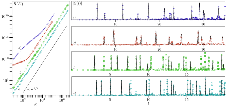
Figure 1: Numerical checks of the fluctuating parts of trace formulae for the two ellipsoids ( a) and b), see text) and the two tori ( c) and d), see text). left: Double logarithmic plot of the integrated squared fluctuations (20) (arbitrary scale), the full line has slope $7/2$. Right: Length spectra of the nodal counting functions (21). The full line is obtained from the trace formulae (Can one count the shape of a drum?) and (Can one count the shape of a drum?) and the points represent the numerical data.

The approximations involved in the above calculation have been tested on an extensive numerical data base for two ellipsoids of revolution defined by the equation $f(x)=R\sqrt{1-x^{2}}$ ($R=2$ in data set a), and $R=1/2$ in data set b)) and for two different tori ($\tau^{2}=2$ in data set c), and $\tau^{2}=\sqrt{2}$ in data set d)). The spectral interval used for the numerical tests included the first $10^{5}$ eigenvalues for the ellipsoids, and the first $4\times 10^{6}$ eigenvalues for the tori. The numerically computed $c(K)$ were fitted to a fourth order polynomial in $\kappa=\sqrt{K}$ and in all cases, the agreement of the two leading coefficients with the asymptotic theory was better than a percent. The oscillating part has been obtained numerically by subtracting the best polynomial fit from the exact $c(K)$. The fluctuating parts of the trace formulae were tested in two ways. The integral of the squared oscillatory part

$$R(K)\approx\int_{0}^{K}{\rm d}K^{\prime}\ c_{\mathrm{osc}}(K^{\prime})^{2}\ .$$ (19)

was computed as a function of $K$, and compared with the theoretical expression which consists of a double sum over periodic geodesics. Simplifying this expression by considering only its diagonal part, one gets the estimate

$$R(K)=\frac{2}{7}K^{\frac{7}{2}}\sum_{\textbf{r}}|a_{\textbf{r}}|^{2}$$ (20)

which scales like $K^{7/2}$. This scaling has been tested and the results are shown in the left part of figure 1. Clearly, the expected power law is reached for sufficiently large values of the counting index $K$. A more stringent test of the trace formula is provided by computing the length spectrum, defined by the properly scaled Fourier transform of $c_{osc}(K)$ with respect to $\kappa=\sqrt{K}$.

$$S(l)=l^{3/2}\!\int_{0}^{\infty}{\rm d}\kappa\ \kappa^{-5/2}c_{\mathrm{osc}}(K=\kappa^{2})e^{-\!\frac{(\kappa-\kappa_{0})^{2}}{\omega}+i\kappa l}\ .$$ (21)

Gaussian windows centered at $\kappa=\kappa_{0}$ and with a width $\propto\sqrt{\omega}$ restricted the data used to be well within the semiclassical domain. The trace formula for the nodal counts predicts pronounced peaks at the scaled lengths $l=l_{\textbf{r}}$ of the periodic geodesics. The right frame in Figure 1 shows a remarkable agreement of the numerical data with the theoretical predictions. This excellent agreement provides further support for the validity of the approximations which were used in the derivation of the two versions of the nodal counts trace formula.

Recent studies GnutzSS ; BandSS have shown that the nodal sequences of isospectral domains are distinct, and can be used to resolve isospectrality. Thus, the geometrical information stored in the nodal sequence is not equivalent to the one stored in the spectral sequence. This result together with the trace formula obtained here motivates further research of the nodal sequence as a tool in spectral analysis.

References

(1)
R. Courant and D. Hilbert,
Methods of Mathematical Physics, Vol I pp 451-465
(Interscience, New York, 1953).
(2) G. Blum, S. Gnutzmann
and U. Smilansky, Phys. Rev. Lett.88, 114101 (2002).
(3)E. Bogomolny and C. Schmit,Phys. Rev. Lett.
88, 114102 (2002).
(4) S. Gnutzmann, U. Smilansky and N. Sondergaard,
J. Phys. A 38 8921 (2005).
(5) R. Band, T. Shapira, and U. Smilansky, to be
published.
(6) M. Berry and M. Tabor,
Proc. Roy. Soc. Lond. Ser. A
356, 375 (1977).