High frequency integrable regimes in nonlocal nonlinear optics.

Abstract

We consider an integrable model which describes light beams propagating in nonlocal nonlinear media of Cole-Cole type. The model is derived as high frequency limit of both Maxwell equations and the nonlocal nonlinear Schrödinger equation. We demonstrate that for a general form of nonlinearity there exist selfguided light beams. In high frequency limit nonlocal perturbations can be seen as a class of phase deformation along one direction. We study in detail nonlocal perturbations described by the dispersionless Veselov-Novikov (dVN) hierarchy. The dVN hierarchy is analyzed by the reduction method based on symmetry constraints and by the quasiclassical $\bar{\partial}-$dressing method. Quasiclassical $\bar{\partial}-$dressing method reveals a connection between nonlocal nonlinear geometric optics and the theory of quasiconformal mappings of the plane.

Key words: Nonlocal Nonlinear Optics, Cole-Cole Media, Phase Singularities, Dispersionless Systems, Quasiconformal Mappings.

1 Introduction.

The optics studies phenomena of the propagation of the electromagnetic waves through a dielectric medium in absence of currents and charges [1]. In such a case the Maxwell equations assume the form

$$\nabla\wedge{\bf H}-\frac{\partial{\bf D}}{\partial t} =0$$ (1.1a)

$$\nabla\wedge{\bf E}+\frac{\partial{\bf B}}{\partial t} =0$$ (1.1b)

$$\nabla\cdot{\bf D} =0$$ (1.1c)

$$\nabla\cdot{\bf B} =0.$$ (1.1d)

where $x,y,z$ are the spatial coordinates, $\nabla=\left(\partial_{x},\partial_{y},\partial_{z}\right)$ is the gradient and $t$ is the time. For sake of simplicity we have set the light speed $c=1$. The vectors ${\bf E}$ and ${\bf B}$ are the electric and magnetic fields respectively, while the displacement vector ${\bf D}$ and the magnetic induction ${\bf H}$ contain the information about the response of the medium when an external electromagnetic field is applied. In general, ${\bf D}$ and H are certain functions of ${\bf E}$ and ${\bf B}$ and they are specified by the so-called constitutive relations. In several physically meaningful cases they can be written down as follows

$${\bf D}=\varepsilon{\bf E}\quad{}{\bf B}=\mu{\bf H},$$ (1.2)

where electric permittivity $\varepsilon$ and the magnetic permeability $\mu$ depend on the coordinates and on the fields. In the case in which $\varepsilon$ and $\mu$ depend at most on the coordinates, the Maxwell equations are linear and provides us with an exhaustive description of a very broad class of phenomena in physics [1, 2, 3].

The nonlinear optics deals with the class of media such that $\varepsilon$ and $\mu$ depend on the fields. In this case, the Maxwell equations are nonlinear and construction of their solutions is, in general, a very challenging problem. In the following, we will focus only on the electric part of the field, assuming the magnetic response to be negligible, i.e. $\mu=1$. This condition is realized in many experimental situations.

By definition, a dielectric medium is referred to as nonlinear if the dielectric function $\varepsilon$ is a certain function of the electric field $\varepsilon=\varepsilon\left({\bf E}\right)$.

The solution of the Maxwell equations for an arbitrary form of the function $\varepsilon$ is, of course, a hard problem. Nevertheless, several very interesting cases, such as quadratic and cubic nonlinearities, are amenable by exact methods. Moreover, they are connected with a relevant phenomenology such as the higher harmonic generation (quadratic nonlinearity) and the soliton production (cubic nonlinearity) [4].

In the present paper we consider a model for light beams propagation in the limit of high frequency. This model can be derived both as high frequency limit of the Maxwell equations and from the nonlinear Schrödinger (NLS) equation which describes paraxial light beams. We will show that it is reasonable to assume the nonlocality to be weak because of the quickly oscillating fields. In particular, we can separate the pure nonlinear contribution from the higher orders nonlocal perturbations. Leading order is represented by the standard eikonal equation. Note that in the standard theory higher order terms contain the amplitude of the electric field as well as the phase $S$ and consequently in virtue of nonlocality and nonlinearity they are rather complicated. Nevertheless, there exist a type of media where it is possible to consider a set of nonlocal perturbations along one direction, say $z$, which are not mixed up with the wave contributions. These are the Cole-Cole media. They are characterized by the Cole-Cole dispersion law for the dielectric function of the form $\varepsilon=\varepsilon_{0}+O(\omega^{-\alpha})$ for $0<\alpha<1$ and $\omega\to\infty$. We would like to stress that a large variety of solid and liquid polar media obeys the Cole-Cole dispersion law [5]. In this case we perform an asymptotic expansion of all fields with respect to the small parameter $\omega^{-\alpha}$ separating first nonlocal correction to the phase $S$ from the higher order wave corrections. In our derivations a suitable slow dependence along $z-$direction is assumed. Nonlocal corrections are described by polynomials in $S_{x}$ and $S_{y}$. In particular, a one-to-one correspondence among nonlocality and polynomials degrees is realized.

In the $\omega\to\infty$ limit separation between the nonlinear response and the nonlocal effects along $z$ suggest to study first the properties of the light beam on the $xy-$plane (transverse equations) and then the “evolution” along $z$. Transverse equations are the two-dimensional eikonal equation and the geometric optics limit of the Poynting vector conservation law. It is shown that for a general class of nonlinear responses obeying the so-called ellipticity condition there exists self-guided light beams. Moreover, several light beam features are determined in terms of the properties of quasiconformal mappings on the plane via the Beltrami equation. Propagation of helicoidal wavefronts and its first degree nonlocal perturbations are also discussed. Thereafter, we focus on the special class of perturbations which preserve the phase inversion symmetry $S\to-S$ similar to the eikonal equation. Such perturbations are shown to be described by an infinite set of integrable nonlinear partial differential equations (PDEs). It is the dispersionless Veselov-Novikov (dVN) hierarchy. First non-trivial equation of the hierarchy can be formally obtained by the slow variable expansion of the Veselov-Novikov equation, which has been introduced in [7] as $(2+1)D$ integrable generalization of Korteweg-de-Vries equation. The dVN hierarchy is of interest since it is treatable by different approaches. More specifically, we discuss the reduction method based on the symmetry constraints. It allows us to reduce the dVN equation to a $1+1-$dimensional hydrodynamic-type system and it is effective for construction of explicit solutions. Moreover, we study the eikonal equation and the dVN hierarchy using the quasiclassical $\bar{\partial}-$dressing method. It provides us with a general approach to construct and analyze the whole hierarchy.

It is worth to note that the quasiclassical $\bar{\partial}-$dressing method establishes a remarkable connection between the nonlocal nonlinear geometric optics and the theory of quasiconformal mappings of the plane.

The paper is organized as follows. The model under consideration is derived from the Maxwell equations in Section 2 and starting with NLS equation in the Section 3. In the Section 4 we analyze the transverse equations in connection with the Beltrami equation and minimal surfaces equation which gives the helicoidal wavefronts. Nonlocal perturbations described by the dVN hierarchy are derived in the Section 5. After a short review about integrable system in the Section 6 we discuss the hydrodynamic-type reductions obtained using the symmetry constraints in Section 7 and the application of the quasiclassical $\bar{\partial}-$dressing method to the eikonal equation and to the dVN hierarchy in Section 8. Some concluding remarks close the paper.

2 The general model.

Let us consider a medium with the magnetic permeability $\mu=1$. In such a case the Maxwell equations (1.1) imply that

$$\nabla\wedge\nabla\wedge{\bf E}+\frac{\partial^{2}{\bf D}}{\partial t^{2}}=0$$ (2.1)

For time oscillating solutions, of the form

$${\bf E}(x,y,z,t) ={\bf E}(x,y,z)\;e^{i\omega t}$$

$${\bf D}(x,y,z,t) ={\bf D}(x,y,z)\;e^{i\omega t},$$

equation (2.1) looks like

$$\nabla\wedge\nabla\wedge{\bf E}-\omega^{2}{\bf D}=0,$$ (2.2)

or, equivalently,

$$\nabla^{2}{\bf E}+\omega^{2}{\bf D}-\nabla\left(\nabla\cdot{\bf E}\right)=0.$$ (2.3)

Once the constitutive relation for ${\bf D}$ is assigned equation (2.3) determines the electric component of the field.

The constitutive relation depends on the physical properties of the medium. Let us assume that the displacement vector ${\bf D}$ can be splitted in a local part ${\bf D}_{L}$ and a nonlocal one ${\bf D}_{N}$ as follows

$${\bf D}={\bf D}_{L}+{\bf D}_{N}$$ (2.4)

where

$${\bf D}_{L} =\varepsilon\left(I(\bf x)\right)\;{\bf E}(\bf x)$$ (2.5)

$${\bf D}_{N} =\int_{\mathbb{R}^{3}}R\left({\bf x}^{\prime}-{\bf x},a(\omega)\right)\;N\left(I({\bf x^{\prime}})\right)\;{\bf E}({\bf x^{\prime}})\;d{\bf x^{\prime}}.$$ (2.6)

The quantity $I=\left|{\bf E}_{0}\right|^{2}$ is the intensity of the electric field, $\varepsilon(I)$ and $N\left(I\right)$ are, respectively, the local and nonlocal nonlinear responses and the function $R({\bf x}-{\bf x^{\prime}})$ is the nonlocal distribution. The parameter $a(\omega)$ governs the width of the nonlocal response in different regimes of the frequency. In particular, in the high frequency limit it is reasonable to assume that the external field is not resonant with the proper oscillations of the particles of the medium in such a way that the response becomes local, i.e.

$$\lim_{\omega\to\infty}R\left({\bf x}^{\prime}-{\bf x},a(\omega)\right)=\delta\left({\bf x}^{\prime}-{\bf x}\right),$$ (2.7)

where $\delta({\bf x}^{\prime}-{\bf x})$ denotes the Dirac $\delta-$function. In order to explain this behavior, one can consider a naive model where the single particle of the medium is described by a one dimensional forced oscillator

$$\ddot{x}+\omega_{0}x=f_{0}\sin\left(\omega t\right).$$ (2.8)

As usual, the dot denotes the total time derivative, $\omega_{0}$ is the proper oscillation frequency of the particle. The left hand side contains the forcing term represented by a linearly polarized electric field oscillating with frequency $\omega$. The solution of equation (2.8) is of the form

$$x=\left\{\begin{aligned} &c_{1}\sin\left(\omega_{0}t\right)+c_{2}\cos\left(\omega_{0}t\right)+\frac{f_{0}}{\omega_{0}^{2}-\omega^{2}}\sin\left(\omega t\right)\quad{}&\omega_{0}\neq\omega\\ &c_{1}\sin\left(\omega_{0}t\right)+c_{2}\cos\left(\omega_{0}t\right)-\frac{f_{0}}{2\omega_{0}}\>t\>\cos\left(\omega_{0}t\right)\quad{}&\omega_{0}=\omega\end{aligned}\right.$$ (2.9)

We remind that we are interested in the non-resonant regime $\omega_{0}\neq\omega$. In this case, it is easy to see that for $\omega\to\infty$ the forcing contribution disappears and the particle behaves as the harmonic oscillator. In this regime one expects that the effect of the external field, up to higher corrections, does not propagate far from the point considered and the response tends to be as local as much $\omega$ is larger.

Substituting the expression (2.4) into equation (1.1c) one gets

$$\nabla\cdot{\bf E}=-\nabla\left(\log\varepsilon\right)\cdot{\bf E}-\frac{\nabla\cdot{\bf D}_{N}}{\varepsilon}.$$ (2.10)

Thus, equation (2.3) takes the form

$$\nabla^{2}{\bf E}+\omega^{2}\left(\varepsilon{\bf E}+{\bf D}_{N}\right)-\nabla\left(-\nabla\log\varepsilon\cdot{\bf E}-\frac{\nabla\cdot{\bf D}_{N}}{\varepsilon}\right)=0.$$ (2.11)

Let us introduce a general model of weak nonlocality. It is given by a nonlocal distribution function of the following form

$$R\left({\bf x}-{\bf x}^{\prime}\right) =\rho_{lmn}\left({\bf x}\right)\delta^{(l,m,n)}\left({\bf x}-{\bf x}^{\prime}\right)$$ (2.12)

where the sum on the repeated indices is assumed. The distributions $\delta^{(l,m,n)}$ are the Dirac $\delta-$function derivatives. They are standardly defined via

$$\int_{\mathbb{R}^{3}}\delta^{(l,m,n)}\left({\bf x}-{\bf x}^{\prime}\right)\;f\left({\bf x}^{\prime}\right)\;d{\bf x}^{\prime}=(-1)^{l+m+n}\frac{\partial^{l+m+n}f({\bf x})}{\partial x_{1}^{l}\partial x_{2}^{m}\partial x_{3}^{n}},$$ (2.13)

where we set ${\bf x}=\left(x_{1},x_{2},x_{3}\right)$.

Using the weak nonlocal distribution (2.12), one can rearrange the expression on the nonlocal contribution ${\bf D}_{N}$ as follows

$${\bf D}_{N}=r^{(0)}({\bf x})N\left(I({\bf x})\right){\bf E}({\bf x})+r^{(1)}_{l}\left({\bf x}\right)\partial_{x_{l}}\left(N\left(I({\bf x})\right)\;{\bf E}({\bf x})\right)$$

$$+r^{(2)}_{lm}\partial_{x_{l}}\partial_{x_{m}}\left(N\left(I({\bf x})\right)\;{\bf E}({\bf x})\right)+r^{(3)}_{lmn}\left({\bf x}\right)\partial_{x_{l}}\partial_{x_{m}}\partial_{x_{n}}\left(N\left(I({\bf x})\right)\;{\bf E}({\bf x})\right)+\dots$$ (2.14)

In principle the coefficients $r^{(n)}$ might depend on the frequency. In particular, we assume the following power dependence

$$r^{(n)}=\frac{\tilde{r}^{(n)}}{\omega^{n}}.$$ (2.15)

We consider a model where the function $N$ depends on the intensity according to the formula

$$N\left(I(\bf x)\right)=\frac{\varepsilon\left(I({\bf x})\right)}{\omega^{\alpha}}$$ (2.16)

where $\alpha$ is a real positive constant parameter.

Under the assumptions mentioned above we perform the geometric optics (semi-classical) limit of equation (2.11). As usual, let us represent the electric field in term of the phase $\tilde{S}$

$${\bf E}\left({\bf x}\right)={\bf E}_{0}\left({\bf x}\right)\;e^{i\omega\tilde{S}\left({\bf x}\right)}.$$ (2.17)

In high frequency limit, $\omega^{-\alpha}$ is the small parameter with respect to which we may consider the following asymptotic expansions

$$I=I_{0}+\omega^{-\alpha}I_{1}+O\left(\omega^{-2\alpha}\right)$$ (2.18)

$$\varepsilon\left(I({\bf x})\right)=\varepsilon_{0}\left(I_{0}({\bf x})\right)+\omega^{-\alpha}\varepsilon_{1}\left(I_{0}({\bf x}),I_{1}({\bf x})\right)+O\left(\omega^{-2\alpha}\right).$$ (2.19)

Evaluating ${\bf D}_{N}$ in the limit of high frequency, one gets

$${\bf D}_{N}\approx\varepsilon_{0}\left(I_{0}({\bf x})\right){\bf E}_{0}({\bf x})\;{\cal D}\;e^{i\omega\tilde{S}({\bf x})},\quad{}\omega\to\infty$$ (2.20)

where

$${\cal D}=\tilde{r}^{(0)}+i\tilde{r}^{(1)}_{l}\;\tilde{S}_{x_{l}}-\tilde{r}^{(2)}_{lm}\;\tilde{S}_{x_{l}}\tilde{S}_{x_{m}}-i\tilde{r}^{(3)}_{lmn}\tilde{S}_{x_{l}}\tilde{S}_{x_{m}}\tilde{S}_{x_{n}}+\dots,$$

$$l,m,n=1,2,3.$$

Using the expression (2.20), we get

$$\nabla\cdot{\bf D}_{N} \approx i\omega\;{\cal D}\;\varepsilon_{0}\left(I_{0}({\bf x})\right)\;{\bf E}_{0}({\bf x})\cdot\nabla\tilde{S}\;e^{i\omega\tilde{S}({\bf x})}$$ (2.21a)

$$\nabla\left(\nabla\cdot{\bf D}_{N}\right) \approx-\omega^{2}\;{\cal D}\;\varepsilon_{0}\left(I_{0}({\bf x})\right)\left({\bf E}_{0}\cdot\nabla\tilde{S}\right)\;\nabla\tilde{S}\;e^{i\omega\tilde{S}({\bf x})}.$$ (2.21b)

Recall that the vector $\nabla\tilde{S}$ is perpendicular to the wavefront and provides us with the light rays direction. Imposing the so-called transversality condition

$${\bf E}_{0}\cdot\nabla\tilde{S}=0$$ (2.22)

we restrict ourselves to the solutions such that the electric field $\bf E$ is perpendicular to the light rays. In this case the terms (2.21a) and (2.21b) do not contribute to the high frequency limit of the equation (2.11).

Moreover, we look for $z-$variable slowly depending solutions of the following form

$$\tilde{S}=kz+S\left(x,y,\tau\right)$$ (2.23)

where $\tau:=z/\omega^{\alpha}$ is the “slow variable”. The high frequency limit of the equation (2.11) at the leading order gives

$$S_{x}^{2}+S_{y}^{2}=4u\left(I_{0}({\bf x})\right)$$ (2.24)

where $4u\left(I_{0}({\bf x})\right)=\varepsilon_{0}\left(I_{0}({\bf x})\right)-k^{2}$.
If the parameter $\alpha$ is such that $0<\alpha<1$ we get an intermediate contribution between the pure geometric optics order and the first correction containing the amplitude of the electric field. In order to calculate it, we note that

$$\tilde{S}_{z}^{2}=\left(k+\omega^{-\alpha}S_{\tau}\right)^{2}=k^{2}+2k\omega^{-\alpha}S_{\tau}+\omega^{-2\alpha}S_{\tau}^{2}$$ (2.25)

where we kept into account that

$$\frac{\partial}{\partial z}=\omega^{-\alpha}\frac{\partial}{\partial\tau}.$$ (2.26)

The $\omega^{2-\alpha}$ order term in equation (2.11) is

$$2kS_{\tau}+\tilde{{\cal D}}\left(x,y,\tau,S_{x},S_{y}\right)\;\varepsilon_{0}+\varepsilon_{1}=0$$ (2.27)

where $\tilde{{\cal D}}$ is a polynomial in $S_{x}$ and $S_{y}$ of the form

$$\tilde{{\cal D}} =\tilde{r}^{(0)}+i\tilde{r}^{(1)}_{l}S_{x_{l}}+ik\tilde{r}^{(1)}_{3}-\tilde{r}^{(2)}_{lm}S_{x_{l}}S_{x_{m}}-k\tilde{r}^{(2)}_{l3}$$

$$-k\tilde{r}^{(2)}_{3m}S_{x_{m}}+\dots,\quad{} l,m=1,2.$$ (2.28)

Resuming, we have derived the following system of equations

$$S_{x}^{2}+S_{y}^{2}=4u\left(I_{0}\right)$$ (2.29a)

$$S_{\tau}=\varphi\left(S_{x},S_{y},I_{0},I_{1},x,y,\tau\right)$$ (2.29b)

where we set

$$\varphi\left(x,y,\tau,S_{x},S_{y}\right)=-\frac{\varepsilon_{0}\left(I_{0}\right)}{2k}\tilde{\cal D}\left(S_{x},S_{y},x,y,\tau\right)-\frac{\varepsilon_{1}\left(I_{0},I_{1}\right)}{2k}.$$ (2.30)

In the construction above, an important rôle is played by the parameter $\omega^{-\alpha}$ with the condition $0<\alpha<1$. It is now natural to ask whether such materials exist in reality. To provide with positive answer let us consider a medium which satisfies the following dispersion law

$$\varepsilon=\varepsilon_{0}+\frac{\tilde{\varepsilon}}{1+\left(2i\omega\right)^{\alpha}},\quad{}0<\alpha<1.$$ (2.31)

The formula (2.31) is referred to as the Cole-Cole dispersion law and it has been found experimentally by the Cole and Cole in 1941 [5]. It is a phenomenoloigical modification of the “classical” Debye law (obtained from the formula (2.31) in the limit case $\alpha=1$). If $\varepsilon_{0}$ and $\tilde{\varepsilon}$ depend on the intensity $I$, the function $\varepsilon_{1}\left(I_{0},I_{1}\right)$ in the expansion (2.19) is

$$\varepsilon_{1}\left(I_{0},I_{1}\right)=\frac{d\varepsilon_{0}}{dI_{0}}\left(I_{0}\right)\;I_{1}+\tilde{\varepsilon}\left(I_{0}\right).$$ (2.32)

Thus, our general model is realizable in the Cole-Cole media.

For sake of simplicity, let us consider a linearly polarized electric field ${\bf E}=E\;\hat{{\bf e}}$, where $\hat{{\bf e}}$ is a constant unit vector and evaluate explicitly the nonlocal term ${\bf D}_{N}=D_{N}\;\hat{{\bf e}}$ in the one-dimensional case

$$D_{N}(x)=\omega^{-\alpha}\int_{-\infty}^{+\infty}R\left(x^{\prime}-x\right)\varepsilon\left(I(x^{\prime})\right)\;E\left(x^{\prime}\right)\;dx^{\prime}$$ (2.33)

If the nonlocal distribution function $R\left(x^{\prime}-x\right)$ is narrow one as it happens in the high frequency limit, one can expand $\varepsilon\left(I(x^{\prime})\right)$ and $E(x^{\prime})$ around the point $x$. So, one gets

$$D_{N}= R_{0}\varepsilon\left(I(x)\right)\;E(x)+R_{1}\left(\varepsilon^{\prime}\left(I(x)\right)\;E(x)+\varepsilon\left(I(x)\right)\;E^{\prime}(x)\right)+$$

$$R_{2}\left(\frac{1}{2}\varepsilon^{\prime\prime}\left(I(x)\right)\;E(x)+\varepsilon^{\prime}\left(I(x)\right)\;E^{\prime}(x)+\frac{1}{2}\varepsilon\left(I(x)\right)\;E^{\prime\prime}(x)\right)\dots$$ (2.34)

where $\epsilon^{\prime}=d\epsilon/dx$ and $\epsilon^{\prime\prime}=d^{2}\epsilon/dx^{2}$

$$R_{n}=\int_{-\infty}^{+\infty}R\left(x^{\prime}-x\right)\left(x^{\prime}-x\right)^{n}\;dx^{\prime}$$

is referred to as $n-$moment of the function $R$. If

$$R_{n}=\frac{r_{n}}{\omega^{n}},$$ (2.35)

in high frequency limit, one gets

$$D_{N}\approx\frac{\varepsilon_{0}E_{0}}{\omega^{\alpha}}\left(r_{0}+ir_{1}S_{x}-\frac{1}{2}r_{2}S_{x}^{2}+\dots\right)\;e^{i\omega S}\quad{}\omega\to\infty.$$ (2.36)

We note that narrower is the nonlocal distribution function $R$ smaller are the higher moments. In this particular case the coefficients $r_{n}$ are related one to another and they are expressed in terms of the fundamental quantity $R$. Thus, the equation of $\omega^{2-\alpha}$ order is

$$S_{\tau}=-\frac{\varepsilon_{0}}{2k}\left(r_{0}+ir_{1}S_{x}-\frac{1}{2}r_{2}S_{x}^{2}+\dots\right)-\frac{\varepsilon_{1}}{2k}.$$ (2.37)

An example of distribution $R$ whose moments are of the form (2.35) is provided by the Gaussian distribution

$$R(x)=\frac{\omega}{\sqrt{\pi}}\;e^{-\omega^{2}x^{2}}.$$ (2.38)

In order to give a complete description of the physical system we should take into account the conservation law of the Poynting vector. The Poynting vector in complex representation is defined as follows [2].

$${\bf P}={\bf E}\wedge{\bf B}^{*}.$$ (2.39)

In the more general case $\mu\neq 1$, $\bf B$ should be replaced by ${\bf H}$ in the formula (2.39).

The conservation law is (see pag. 35 in the reference [1])

$$\nabla\cdot{\bf P}=0.$$ (2.40)

Equation (1.1b) for time-oscillating fields looks like as follows

$$\nabla\wedge{\bf E}+i\omega{\bf B}=0.$$ (2.41)

Using the representation

$${\bf E}={\bf E}_{0}\;e^{i\omega\tilde{S}},\quad{}{\bf B}={\bf B}_{0}\;e^{i\omega\tilde{S}},$$

one gets

$$\nabla\wedge{\bf E}_{0}+i\omega\nabla\tilde{S}\wedge{\bf E}_{0}=i\omega{\bf B}_{0}.$$ (2.42)

The leading order in high frequency limit gives

$${\bf B}_{0}=\nabla\tilde{S}\wedge{\bf E}_{0}.$$ (2.43)

Thus, we have the following approximation of the Poynting vector

$${\bf P}={\bf E}_{0}\wedge{\bf B}_{0}={\bf E}_{0}\wedge\left(\nabla\tilde{S}\wedge{\bf E}_{0}^{*}\right)=$$

$$\left({\bf E}_{0}\cdot{\bf E}_{0}^{*}\right)\;\nabla\tilde{S}-\left({\bf E}_{0}\cdot\nabla\tilde{S}\right)\;{\bf E}_{0}^{*}$$

In virtue of the transversality condition (2.22) one finally has

$${\bf P}=I\;\nabla\tilde{S}.$$ (2.44)

where $I=\left|{\bf E}_{0}\right|^{2}$. Note that ${\bf P}$ is parallel to the gradient of the phase $\nabla S$. Using the expression (2.44) in (2.40), one obtains

$$\nabla I\cdot\nabla\tilde{S}+I\nabla^{2}\tilde{S}=0.$$ (2.45)

Due to the slow dependence on the variable $z$, for phases of the form (2.23) and the asymptotic expansion $I=I_{0}+\omega^{-\alpha}I_{1}+\dots$, equation (2.45) becomes

$$I_{0}\left(S_{xx}+S_{yy}\right)+I_{0x}S_{x}+I_{0y}S_{y}=0$$ (2.46a)

$$I_{1}\left(S_{xx}+S_{yy}\right)+I_{1x}S_{x}+I_{1y}S_{y}+kI_{0\tau}=0.$$ (2.46b)

The system (2.46) has to be considered together with the system for the phase (2.29).

The properties of present model have to be investigated by the joint analysis of the system (2.29) and the system (2.46). In our discussions we will separate the compatibility analysis of the transverse equation (2.29a) and (2.46a) from the “evolution” equations (2.29b) and (2.46b).

3 Paraxial light beams.

3.1 The nonlocal NLS equation.

Many phenomenological models are based on the so-called nonlocal NLS equation [8, 9, 10, 11, 12, 13, 14, 16, 17]. It describes paraxial light beams in nonlinear (and also nonlocal) media. In the present section we discuss the connection between the high frequency model discussed above and the nonlocal NLS equation.

Let us consider a displacement vector of the form

$${\bf D}=\sigma{\bf E}+\sigma^{3}{\bf D}^{(3)},$$ (3.1)

where $\sigma$ is a constant parameter. The paraxial approximation in equation (2.3) is usually performed by the consideration of the slow variations of a small-amplitude electric field (or formally by the substitutions)

$$\left(\partial_{x},\partial_{y},\partial_{z}\right)\to\left(\sigma\partial_{x},\sigma\partial_{y},\sigma^{2}\partial_{z}\right),\quad{}{\bf E}\to\sigma{\bf E}\;e^{i\omega z}.$$

The leading nontrivial order in equation (2.3) is

$$2i\omega\frac{\partial{\bf E}}{\partial z}+\nabla_{\bot}^{2}{\bf E}+\omega^{2}{\bf D}^{(3)}=0,$$ (3.2)

where $\nabla_{\bot}=\left(\partial_{x},\partial_{y}\right)$. For a general nonlocal nonlinear medium we can write

$${\bf D}^{(3)}=\int_{\mathbb{R}^{3}}R\left({\bf r^{\prime}}-{\bf r};a\right)\;N\left(I({\bf r^{\prime}})\right){\bf E}({\bf r^{\prime}})\;d^{3}{\bf r^{\prime}}$$ (3.3)

where ${\bf r}=\left(x,y,z\right)$. We use the notation ${\bf D}^{(3)}$ to recall that, in the case of a local Kerr medium, the relation (3.3) is reduced to the cubic nonlinearity which is associated with the standard NLS equation [4]. The distribution $R({\bf r}^{\prime}-{\bf r};a)$ characterizes the nonlocal response around the point ${\bf r}$ and $a$ is the “width” parameter (in the following it will be assumed to be depending on the frequency $\omega$). $N(I)$ is a certain nonlinear response depending on the intensity of the electric field $I=\left|{\bf E}\right|^{2}$.

We note that due to the paraxial approximation the nonlocal response along $z$ can be neglected. As illustrative example to explain this fact let us consider a Gaussian nonlocal response

$$R\left({\bf r}^{\prime},{\bf r}\right)=\frac{1}{\left(2\pi\right)^{\frac{3}{2}}}\;e^{-\left|{\bf r}^{\prime}-{\bf r}\right|^{2}}$$ (3.4)

where $\left|{\bf r}\right|^{2}=x^{2}+y^{2}+z^{2}$. Due to the paraxial approximation we take into account of slow dependence on the variable $z$ by the substitution $z\to\epsilon^{-1}z$

$$\lim_{\epsilon\to 0}\frac{1}{\epsilon(2\pi)^{\frac{3}{2}}}\;e^{\frac{(z^{\prime}-z)^{2}}{\epsilon^{2}}}\;e^{(x^{\prime}-x)^{2}+(y^{\prime}-y)^{2}}=\frac{1}{2\pi}\;\delta\left(z^{\prime}-z\right)\;e^{(x^{\prime}-x)^{2}+(y^{\prime}-y)^{2}}.$$ (3.5)

The Dirac $\delta-$function in the left hand side of (3.5) implies that the response along the direction $z$ becomes local. Thus, with the use of the distribution (3.5) in the general definition of ${\bf D}^{(3)}$ the $3$D integral is reduced to a $2-$dimensional one

$${\bf D}^{(3)}=\int_{-\infty}^{+\infty}\int_{-\infty}^{+\infty}R\left(x^{\prime}-x,y^{\prime}-y,a\right)\;N\left(I(x,y,z)\right)\;{\bf E}(x,y,z)\;dx\;dy.$$ (3.6)

The model considered above, can be further simplified under suitable assumptions on the widths of the nonlocal distribution $R$ and the nonlinear response $N(I)$. For sake of simplicity we focus on the $1+1-$dimensional case

$$2i\omega\frac{\partial{\bf E}}{\partial z}+\frac{\partial^{2}{\bf E}}{\partial x^{2}}+\omega^{2}{\bf D}^{(3)}=0$$ (3.7)

where

$${\bf D}^{(3)}=\int_{-\infty}^{+\infty}R(x-x^{\prime};a)\;N\left(I(x^{\prime})\right)\;{\bf E}(x^{\prime})dx^{\prime}.$$ (3.8)

Let us define the width $\delta R$ of the nonlocal distribution $R\left(x-x^{\prime};a\right)$ as the minimum such that

$$R\left(x-x^{\prime};a\right)\simeq 0,\quad{}\forall x^{\prime}\notin\left[x-\delta R,x+\delta R\right].$$ (3.9)

Of course, $\delta R$ depends on the width parameter $a$. Similarly, we can introduce the widths $\delta E$ and $\delta N$ of the electric field and the nonlinear response respectively. Suppose they satisfy the following conditions

$$\delta R\sim\delta N,\quad{}\delta R<<\delta E.$$ (3.10)

Moreover, we assume the nonlinear response $N(I)$ to be of the form

$$N\left(I(x)\right)=\tilde{N}\left(X\right),$$ (3.11)

where $X=\gamma\>x$ and $\gamma\propto 1/\delta N$. Expanding ${\bf E}(x^{\prime})$ and $N\left(I(x^{\prime})\right)$ in Taylor series around $x$, one gets the following approximation of the formula (3.8)

$${\bf D}^{(3)}\simeq\left(\int_{-\infty}^{+\infty}R\left(x-x^{\prime};a\right)N\left(I(x^{\prime})\right)dx^{\prime}\right){\bf E}(x),$$ (3.12)

where we kept into account that due to equation (3.11) higher orders of the expansion of $N\left(I(x)\right)$ are not negligible. Note that the formula (3.12), in the case of nonlocal Kerr-type medium, leads to the nonlocal nonlinear Schrödinger equation discussed in the paper [11].

For instance, given a bell-shape electric field ${\bf E}={\bf E}_{0}\;\exp\left[-x^{2}/2\sigma^{2}\right]$, a nonlinear response of the form $N(I)=I^{\alpha}=\left|{\bf E}_{0}\right|^{2\alpha}\;\exp\left[-\left(\gamma x\right)^{2}/{2\sigma^{2}}\right]$, where $\gamma=\sqrt{2\alpha}$, satisfies the condition (3.11). Nevertheless, it is easy to see that only the validity of relations (3.10) is sufficient to obtain the model (3.12). For instance, for ${\bf E}={\bf E}_{0}/\cosh^{2}(x)$ and $N\left(I\right)=I^{\alpha}$, condition (3.10) is verified for $\alpha$ large enough. Finally, we note that it is straightforward to generalize the previous considerations to construct a more general $(2+1)$D model.

3.2 High frequency regimes.

Now, we discuss the above in high frequency regime.

With the representation

$${\bf E}={\bf E}_{0}\;e^{i\omega\tilde{S}(x,y,z)},$$

the NNLS equation takes the form

$$2\tilde{S}_{z}+\left(\nabla_{\bot}\tilde{S}\right)^{2}=N_{0}\left(I_{0}\left(x,y,z\right)\right),$$ (3.13)

where $\nabla_{\bot}=\left(\partial_{x},\partial_{y}\right)$ and $N_{0}(I_{0})$ is the high frequency limit of the intensity law

$$\mathop{\rm\lim}\limits_{\omega\to\infty}N\left(I\right)=N_{0}\left(I_{0}\right)$$

Paraxial approximation of the Poynting vector conservation law (2.40) at the leading order on $\sigma$ gives the following equation on the $xy-$plane

$$\nabla_{\bot}I\cdot\nabla_{\bot}\tilde{S}+I\nabla_{\bot}^{2}\tilde{S}=0.$$ (3.14)

An analysis of the $(1+1)$D reduction of the couple of the equations (3.13) and (3.14) suggests that possible stable light beams (in this specific regime) exists only in $(2+1)D$. Indeed, the following example shows that the bell-shape initial beam profiles are no longer preserved.

If $S$ in equations (3.13) and (3.14) does not depend on the variable $y$, one has

$$2\tilde{S}_{z}+\tilde{S}_{x}^{2}=N_{0}\left(I_{0}\right)$$ (3.15a)

$$I_{0}\tilde{S}_{xx}+I_{0x}\tilde{S}_{x}=0.$$ (3.15b)

Integrating equation (3.15b), one gets

$$\tilde{S}_{x} =\frac{\gamma_{0}}{I_{0}}$$ (3.16a)

$$\tilde{S}_{z} =\frac{1}{2}\left(N_{0}(I_{0})-\frac{\gamma_{0}^{2}}{I_{0}^{2}}\right),$$ (3.16b)

where $\gamma_{0}$ is an arbitrary real constant. In virtue of $S_{xz}=S_{zx}$ one obtains

$$I_{0z}+\left(\frac{I_{0}^{2}N_{0}^{\prime}(I_{0})}{2\gamma_{0}}+\frac{\gamma_{0}}{I_{0}}\right)I_{0x}=0,$$ (3.17)

where $N^{\prime}_{0}:=\frac{dN_{0}}{dI_{0}}$. General solution of equation (3.17), calculated by the characteristics method [15], is provided by the following implicit relation

$$x-\left(\frac{I_{0}^{2}N^{\prime}(I_{0})}{2\gamma_{0}}+\frac{\gamma_{0}}{I_{0}}\right)-\Phi\left(I_{0}\right)=0$$ (3.18)

where $\Phi$ is an arbitrary function of its argument. It is assigned by the initial profile of the intensity

$$I_{0}\left(x,0\right)=\Phi^{-1}\left(x\right).$$ (3.19)

It is well known [18] that equations of type (3.17) exhibit breaking wave phenomena for finite $z$. For example, a smooth initial profile, such that $I_{0}\to 0$ for $x\to\pm\infty$ breaks at finite $z$ where $I_{0x}\to\infty$.

Let us now consider a $(2+1)$D model for the following class of solutions

$$\tilde{S}=kz+S\left(x,y,\tau\right),$$ (3.20)

where $k$ is a real constant and $\tau=\omega^{\alpha}z$ (with $\alpha>0$). A class of nonlocal perturbations with respect to the slow variable $\tau$ will be discussed in the following subsection. Under these assumptions equations (3.13) and (3.14) assume the following form

$$S_{x}^{2}+S_{y}^{2}=4u\left(I_{0}(x,y)\right)$$ (3.21a)

$$I_{0}\left(S_{xx}+S_{yy}\right)+I_{0x}S_{x}+I_{0y}S_{y}=0$$ (3.21b)

where $4u(I_{0})=\tilde{N}_{0}(I_{0})-2k$. We kept into account that due to the rule

$$\frac{\partial}{\partial z}=\omega^{-\alpha}\frac{\partial}{\partial\tau}$$

$z-$derivatives do not contribute in the limit $\omega\to\infty$. We note also that $I_{0}$ is the leading order term of the $\omega^{-\alpha}-$asymptotic expansion of the intensity

$$I(x,y,z)=I_{0}(x,y,\tau)+\omega^{-\alpha}I_{1}(x,y,\tau)+\dots\;.$$

One refers to the functional dependence among $u$ and $I_{0}$ as intensity law. It is determined by the specific physical properties of the medium. Note that once $u(I_{0})$ is given, the system (3.21) is overdetermined. Its consistency condition will be discussed in the next section.

3.3 Nonlocal perturbations.

Let us consider a model for which the nonlocal nonlinear contribution to the displacement vector is of the following form

$${\bf D}^{(3)}=\varepsilon{\bf E}+{\bf D}_{N}$$ (3.22)

where

$${\bf D}_{N}=\int_{\mathbb{R}^{2}}\;R\left({\bf r}^{\prime}-{\bf r},\omega\right)\;N\left(I({\bf r}^{\prime},z)\right){\bf E}({\bf r},z)d{\bf r}^{\prime}$$

In particular, we are interested in the construction of a special class of weak nonlocal perturbations given by a nonlocal distribution function of the form

$$R\left({\bf r}-{\bf r}^{\prime},\omega\right)=\sum_{l,m=0}^{M}R_{l,m}\left({\bf r},\omega\right)\;\delta^{(l,m)}\left({\bf r}-{\bf r}^{\prime}\right),$$ (3.23)

where ${\bf r}=\left(x,y\right)$ the distributions $\delta^{(l,m)}$ are defined by (2.13) and $M$ is an arbitrary integer referred to as nonlocality degree. As a consequence one gets

$${\bf D}_{N}=\sum_{l=1}^{2}c_{n}\frac{\partial{\bf E}}{\partial x_{l}}+\sum_{l,m=1}^{2}c_{l,m}\frac{\partial^{2}{\bf E}}{\partial x_{l}\leavevmode\nobreak\ \partial x_{m}}+\dots\;\;\;.$$ (3.24)

Using the following asymptotic expansions on $\omega^{-\alpha}$

and proceeding similarly to the previous section for a Cole-Cole medium (2.31), one gets from the NNLS equation in the leading orders $\omega^{2}$ and $\omega^{2-\alpha}$ the following system

$$S_{x}^{2}+S_{y}^{2}=4u,$$ (3.25a)

$$S_{\tau}=\varphi(S_{x},S_{y},x,y,\tau)$$ (3.25b)

where $4u=\varepsilon_{0}-2k$ and the function $\varphi$ is a polynomial in $S_{x}$ and $S_{y}$. Equation (3.25a) is the well known eikonal equation in two-dimensions. The function $\varphi$ in equation (3.25b), in virtue of expression (3.24), is an $M$-degree polynomial in $S_{x}$ and $S_{y}$ and it describes an $M$-degree nonlocal response. Moreover, if we require that equation (3.25b) possesses the phase inversion symmetry ($S\to-S$) just like the eikonal equation, the function $\varphi$ must contain only odd degree terms in $S_{x}$ and $S_{y}$. We note also that the system of equations (3.25) has been derived first directly from the Maxwell equations [14, 16].

In local case we have

$$\varphi=\varphi(z),\quad{}u=u(x,y),$$ (3.26)

where $\varphi$ and $u$ are certain function of their arguments. For a first degree nonlocality we have

$$\varphi=\alpha_{1}S_{x}+\alpha_{2}S_{y},\quad{}$$ (3.27)

and $u$ must satisfy the following linear equation

$$u_{z}=\left(\alpha_{1}u\right)_{x}+\left(\alpha_{2}u\right)_{y},$$ (3.28)

where $\alpha_{1}$ and $\alpha_{2}$ are harmonic conjugate functions, that is they satisfy the Cauchy-Riemann conditions $\alpha_{1x}$ $=$ $\alpha_{2y}$ $\alpha_{1y}$ $=$ $-\alpha_{2x}$.

4 Transverse equations.

The compatibility of the system of equations for the phase (2.29) and intensity (2.46) results to be highly nontrivial problem. More specifically, one can see that it is not consistent for arbitrary intensity law. The construction presented above suggest to separate the compatibility analysis on the $xy-$plane from the evolution along the $z-$direction. We will study the system of equations (2.29a) and (2.46a) for a general form of the intensity law and then we will discuss the “evolution” of the solutions with respect to the variable $\tau$.

4.1 Elliptic intensity laws.

Let us assume the function $u(I_{0})$ to be invertible. Note that for various physically meaningful models such as the Kerr-type media

$$u=I_{0}^{\gamma},\quad{}\gamma>0$$ (4.1)

and logarithmic saturable media

$$u=\log\left(1+I_{0}/I_{0t}\right)$$ (4.2)

where the constant $I_{0t}$ is the so-called threshold intensity, intensity law is the invertible one.

Then, we can consider the function $I_{0}=I_{0}(u)$. We refer to it as inverse intensity law. Since

$$\nabla_{\bot}I_{0}=I_{0}^{\prime}\nabla_{\bot}u$$

where $I_{0}^{\prime}=dI_{0}/du$, the system of equations (2.29a)and (2.46a) (or (3.21)) looks like as follows

$$S_{x}^{2}+S_{y}^{2}=4u$$ (4.3a)

$$I_{0}\left(S_{xx}+S_{yy}\right)+I_{0}^{\prime}\left(u_{x}S_{x}+u_{y}S_{y}\right)=0.$$ (4.3b)

Substituting the expression for $u$ from (4.3a) into (4.3b), we obtain the following second order partial differential equation

$$AS_{xx}+BS_{yy}+2CS_{xy}=0,$$ (4.4)

where by definition $J_{0}=\log I_{0}$ and

$$A=J_{0}\;^{\prime}S_{x}^{2}+2,\quad{}B=J_{0}\;^{\prime}S_{y}^{2}+2,\quad{}C=J_{0}\;^{\prime}S_{x}S_{y}.$$ (4.5)

The equations of the form (4.4) are well studied in mathematics (see e.g. [19] and references therein). Their properties are critically depending on the signature of the discriminant

$$\Delta=AB-C^{2}.$$ (4.6)

In particular, one can distinguish three cases, elliptic ($\Delta>0$), parabolic ($\Delta=0$) and hyperbolic ($\Delta<0$). In what follows, we will focus on the elliptic case motivated by the fact that the intensity law for Kerr-type (4.1) and logarithmic saturable media (4.2) satisfy the ellipticity condition $\Delta>0$ uniformly. We remark that these models are very relevant in practical applications since they are associated with the propagation of stable spatial solitons [20, 21]

We would like to emphasize that elliptic second order nonlinear equations of the form (4.4) possess several remarkable analytical and geometrical properties (see e.g. [19, 22, 23, 24, 25]). An interesting class of solutions of equation (4.4) is provided by the Beltrami equation which is well known and well studied in the theory of elliptic systems of PDEs and in the theory of quasiconformal mappings[24, 25]. Let us introduce the complex variable $z=x+iy$ (it should not be confused with real variable associated with the $z-$axis) and the complex gradient $w=S_{x}-iS_{y}$. In these notations equation (4.4) takes the form

$$aw_{z}+bw_{\bar{z}}+\bar{a}\bar{w}_{\bar{z}}+\bar{b}\bar{w}_{z}=0,$$ (4.7)

where

$$a=\frac{1}{2}\left(A-B+2iC\right),\quad{}b=\frac{1}{2}\left(A+B-2iC\right).$$ (4.8)

It is immediate to verify that if $w$ satifies the, so-called, nonlinear Beltrami equation

$$w_{\bar{z}}=\mu\left(w,\bar{w}\right)w_{z},\quad{}\mu=-\frac{a}{b}.$$ (4.9)

then it is also a solution of equation (4.7). It is easy to verify that ellipticity condition $\Delta>0$ implies $\left|\mu\right|<1$. Function $\mu$ possesses a remarkable geometrical meaning being the complex dilatation of the quasiconformal mapping $w$.

Thus, the evolution of a light beam profile along the direction $\tau$ turns out to be described by suitable deformations of quasiconformal mappings.

More specifically, let us consider an input light beam profile such that $I_{0}\neq 0$ inside a simply connected domain $G$ and $I_{0}=0$ onto the smooth boundary $\Gamma$ of $G$ and outside it. Set $u_{0}=u(I_{0}=0)$. Writing down the eikonal equation (3.21a) in terms of $w$ and $z$, one gets

$$w(z)\bar{w}(z)=4u.$$ (4.10)

From equation (4.10) one gets $\left|w\right|=2\sqrt{u_{0}}$ for $z\in\Gamma$, that is $\Gamma$ is mapped on the $2\sqrt{u_{0}}$-radius circle. Assuming $w$ to be assigned in such a way that, for instance, $w(0)=0$, where $0\in G$, and the variation of the argument of the complex number $w$ around $\Gamma$ is $\Delta_{\Gamma}\arg w=2\pi$, it can be proven that $w$ is a homeomorphic mapping of domain $G$ onto $2\sqrt{u_{0}}-$radius disk $\Gamma\;^{\prime}$ [22]. Of course, mapping $w$ preserves the topology of domain $G$. In virtue of the assumption (3.20) the wavefront evolves according to the equation

$$\omega^{-\alpha}k\tau+S(x,y,\tau)=\textup{const}.$$ (4.11)

We observe that the mapping $w=S_{x}-iS_{y}=\left(S_{x},-S_{y}\right)$ can be also regarded as a two-dimensional vector field on the $z-$plane associated with transverse components of the wavefront normal unit vector

$${\bf n}=\frac{\nabla\tilde{S}}{|\nabla\tilde{S}|}=\left(\frac{S_{x}}{\sqrt{k^{2}+4u}},\frac{S_{y}}{\sqrt{k^{2}+4u}},\frac{1}{\sqrt{k^{2}+4u}}\right).$$ (4.12)

We remind that the vector ${\bf n}$ is, by definition, parallel to the Poynting vector. This means that the mapping $w$ encodes information about light-rays distribution around direction $\tau$. For example, let us consider the mapping given in figure 4.1. Curves $\Gamma$ and $\Gamma^{\prime}$ are oriented leaving domain on the right hand side. Under the assumptions mentioned above, there exists a homeomorphism $w$ of domain $G$ onto $G^{\prime}$ acting in such a way that $w(s_{1},0)=(-1,0)$, $w(0,s_{2})=(0,1)$ and $w(-s_{3},0)=(1,0)$. Consequently, the normal unit vector to wave-front on the boundary $\Gamma$ is oriented in such a way that the light rays lie inside the rectangle circumscribing the domain $G$ (see figure 4.1). Recall that $y$-component of $w$ reverse $y$-component of $\bf{n}$. Then, this mapping describes a light beam ‘trapped’ around the direction $\tau$. Conversely, if $w(s_{1},0)=(1,0)$, $w(0,s_{2})=(0,-1)$ and $w(-s_{3},0)=(0,-1)$ radiation spreads transversely far from $\tau-$direction. Note also that in both cases homeomorphism $w$ is sense-reversing. If we consider a sense-preserving mapping such as, for instance, $w(s_{1},0)=(1,0)$, $w(0,s_{2})=(0,1)$ and $w(-s_{3},0)=(-1,0)$, the beam spreads along $x-$direction and tends to be trapped along $y-$axis (see figure 4.2). The boundary conditions and the orientation of the mapping allows us to control strongly the properties of the light beam.

We emphasize, finally, that all of these observations can be generalized to the case of arbitrary $n-$connected domains. They could be used for description of interacting light beams.

Figure 4.1: Sense-reversing mappings (solid line) describe beams which tend to be confined inside the rectangle or scattered (dashed line) outside it.

Figure 4.2: For the sense-preserving mapping the light beam spreads along $x-$direction and tends to be trapped along $y-$direction.

Another class of solutions of equation (4.7) can be obtained solving the equation

$$bw_{\bar{z}}+\bar{a}\bar{w}_{\bar{z}}=0.$$ (4.13)

Introducing the reciprocal coordinates by inversion of the system

$$\begin{aligned} z&=z(w,\bar{w})\\ \bar{z}&=\bar{z}(w,\bar{w}),\end{aligned}$$ (4.14)

one converts equation (4.13) into the form of the linear Beltrami equation

$$z_{\bar{w}}=\nu(w,\bar{w})z_{w},$$ (4.15)

where $\nu(w,\bar{w})=-\bar{a}/b$ and, due to ellipticity, $|\nu|<1$. The advantage of consideration of equation (4.13) in reciprocal coordinates is that the Beltrami equation is linear and it can be solved explicitly for different choices of the intensity law. Moreover, it is well known that several theorems in analytic functions theory can be rigorously generalized to the quasi-analytic functions which are the solutions of equation (4.15) (see e.g. Ref. [24]). In particular, a generalization of so-called Liouville theorem (Vekua’s theorem) holds. If $z=z(w,\bar{w})$ is bounded on whole $w-$plane and satisfies the linear Beltrami equation (4.15) it can be shown that $z(w,\bar{w})\equiv\textup{constant}$ [26]. We stress that for the constant solution, mapping from $w-$to$-z-$plane is singular and reciprocal transformation (4.14) is not defined. Then, any non-trivial solution of equation (4.15) must be singular somewhere on the complex plane and different type of singularities can occur, such as poles, essential singularities, singularities of the derivatives etc.

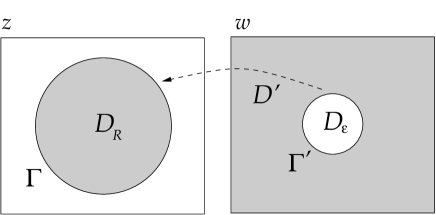
Figure 4.3: Homeomorphic mapping from the exterior of $D_{\epsilon}$ on $D_{R}$ such that $\Gamma^{\prime}$ goes onto $\Gamma$. Light rays associated with the points outside $D_{R}$ are parallel to the $z-$axis as much as $\epsilon$ is small.

As illustrative example, we focus our attention on a solution $z(w,\bar{w})$ which have a simple pole at $w=0$. As discussed above, one can always consider a homeomorphism from $D^{\prime}=\mathbb{C}\setminus D_{\epsilon}$ to $D_{R}$, where $D_{\epsilon}$ is a disk of arbitrarily small radius $\epsilon$ on the $w-$plane and $D_{R}$ is the $R$-radius disk on the $z-$plane, mapping the boundary of $D_{\epsilon}$ on the boundary of $D_{R}$. Inverse mapping $w:\;D_{R}\to D^{\prime}$, constructed in such a way, can be used to describe a beam “confined”around $\tau-$axis. Indeed, the transverse component of the vector ${\bf n}$ outside $D_{R}$ are arbitrarily small. Hence, the light rays can be settled down parallel to the $\tau-$axis with arbitrary accuracy. So, the beam results to be self-guided around $\tau$ as much as disk $D_{\epsilon}$ is small.

Coming back to nonlinear Beltrami equation (4.9), we expect that for “mild enough” complex dilatations $\mu$, Vekua’s theorem still holds. In these cases, the only one bounded solution on whole $z-$plane is $w=\textup{constant}$. In many physical situations, the intensity distribution on the $z-$plane, at certain $\tau$, goes to zero for $z\to\infty$, or equivalently, one can says that intensity vanishes outside a big enough $R-$radius disk $D_{R}$. Thus, outside $D_{R}$, refractive index assumes a constant value $u=u_{0}$ and the solutions of eikonal equation (3.21a) is

$$S=c_{0}x+c_{1}y+c_{3},$$ (4.16)

where $c_{0}$, $c_{1}$ and $c_{3}$ are constants and the condition $c_{0}^{2}+c_{1}^{2}=4u_{0}$ holds. For a paraxial beam we have $c_{0}=c_{1}=0$. As the consequence $w=S_{x}-iS_{y}=c_{0}-ic_{1}=0$ and, of course it satisfies Beltrami equation in $\mathbb{C}\setminus D_{R}$. In virtue of Vekua’s theorem, the only one bounded solution is $w\equiv 0$. Then, any non-trivial solution must be singular somewhere on the plane. In our example, wavefront is approximately plane for $z\in\mathbb{C}\setminus D_{R}$ and possesses singularity inside $D_{R}$.

In the next subsection we will discuss the so-called optical vortices obtained from equation (4.4) assuming the phase to be a harmonic function on the $xy-$plane. We will see that, in this case, equation (4.4) is equivalent to the minimal surfaces equation. We refer to this class of solutions as minimal sector in order to distinguish it from the Beltrami sector which is associated with the solutions of equations (4.9) and (4.15).

4.2 Helicoidal wavefronts.

The successive approximations method is a general approach to solve the linear Beltrami equation (it has been demonstrated by Tricomi [27]). Nevertheless, calculation of exact ‘explicit’ solutions can be the difficult task and the chances of success strongly depend on the form of the complex dilatation. Incidentally, we note that solutions possessing cylindrical symmetry such that

$$S=S(r),\quad{}u=u(r),\quad{}r=\sqrt{x^{2}+y^{2}},$$ (4.17)

are not compatible with intensity law. It is straightforward to verify that equations (3.21) along with assumptions (4.17) imply that intensity depends explicitly on $z-$axis distance $r=\sqrt{x_{2}+y^{2}}$

$$I_{0}=\frac{1}{2cr\sqrt{u}},$$ (4.18)

where $c$ is an arbitrary constant.

Here, we will consider the solutions of equation (4.4) connected with the, so-called, minimal surfaces. The minimal surface equation looks like as follows (see e.g. Ref. [28])

$$\left(1+S_{y}^{2}\right)S_{xx}+\left(1+S_{x}^{2}\right)S_{yy}-2S_{x}S_{y}S_{xy}=0.$$ (4.19)

We restrict ourselves to the class of solutions of equation (4.4) which are also harmonic on the $xy-$plane, that is

$$S_{xx}+S_{yy}=0.$$ (4.20)

Using the condition (4.20) in equation (4.4), one gets the equation

$$S_{x}^{2}S_{xx}+S_{y}^{2}S_{yy}+2S_{x}S_{y}S_{xy}=0,$$ (4.21)

for any elliptic intensity law. It is straightforward to check that equations (4.21) and (4.19) coincide for harmonic solutions. In other words, a class of solutions of equation (4.4), whatever is the inverse intensity law $I_{0}=I_{0}(u)$, is just given by the class of the harmonic minimal surfaces. An important result for us is that the only non-trivial harmonic minimal surface in Cartesian coordinates is the helicoid [28]. It can be written as follows

$$S=K\arctan\left(\frac{\beta\tau+y}{x}\right),$$ (4.22)

where $K$ is an arbitrary constant. One can check that the function $S$ given by (4.22) satisfies equations (4.19), (4.20) and (4.21) simultaneously. Equation of corresponding wavefronts is

$$\tilde{S}\equiv\omega^{\alpha}\tau+K\arctan\left(\frac{\beta\tau+y}{x}\right)=\textup{const},$$ (4.23)

where the constant $K$ is the “pitch” of the helicoid. In particular, the expression (4.23) describes the edge-screw dislocations discussed first time experimentally by Brynghdal in 1973 [29] and theoretically by Nye and Berry [30] in 1974. We highlight that helicoidal wavefronts exist in both linear and (nonlocal) nonlinear regimes. They are associated with singularity of the phase (phase defects) which appears as topological defects of the interferograms. These class of phase defects has important phenomenological consequences connected to the optical vortices [31, 32, 33, 34] (see also Refs. [35, 36] and references therein). If we assume, for simplicity, $\beta=0$ in (4.22), one has the pure screw dislocations. The complex gradient associated with the helicoid

$$w=-i\frac{K}{z}$$ (4.24)

is a meromorphic function on $z$ with the simple pole singularity at the origin. Nevertheless, normal vector to the wavefront, whose components coincides (up to a sign) with real and imaginary parts of $w$, is not defined. Indeed, vector $w=(S_{x},-S_{y})$ has no limit as $\left(x,y\right)\to 0$. Figure 4.4 shows examples of helicoidal wavefronts (4.23) usually parametrized as follows

$$x=v\cos t,\quad{}y=v\sin t,\quad{}z=Kt.$$ (4.25)

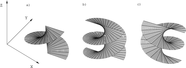
Figure 4.4: Helicoidal structures of wavefront around $\tau-$axis: a) one-start right-screw ($K=1$); b) two-start right screw ($K=1$); c) two-start left screw ($K=-1$).

One-start helicoid shown in figure 4.4a is obtained for $0<v<+\infty$; two-start helicoids shown in figure 4.4b,c are obtained for $-\infty<v<+\infty$. Refractive index

$$u=\frac{K^{2}}{4(x^{2}+y^{2})}$$ (4.26)

has cylindrical symmetry around $\tau-$axis and displays divergence at $z=0$. This means that around the origin geometric optics approximation fails and wave effects become relevant. In particular, necessary condition for the existence of singular wavefronts is that intensity vanishes where phase function is singular [30]. Indeed, in this region the interference phenomenon is no more negligible and can realize this condition.

It is interesting to evaluate the effect of the present class of nonlocal perturbations

$$S_{\tau}=\varphi\left(S_{x},S_{y},x,y,\tau\right)$$

discussed in the sections 2 and 3, on the pure ($\beta=0$) helicoidal wavefront (4.22). In particular we note that the solution (4.22) of the equation (4.21) is defined up to an additive arbitrary function of $\tau-$variable $\psi(\tau)$, such that $\psi^{\prime}=\varphi(\tau)$. Then, one has

$$S=K\arctan\left(y/x\right)+\psi(\tau).$$

Let us observe that the function $\psi(\tau)$ is specified by the function $\varphi$ evaluated on the helicoid. For example, in the case of the first degree nonlocality one has (see equations (3.27) and (3.28))

$$\begin{aligned} \psi^{\prime}(\tau)&=\alpha_{1}S_{x}+\alpha_{2}S_{y}\\ u_{\tau}&=\left(\alpha_{1}u\right)_{x}+\left(\alpha_{2}u\right).\end{aligned}$$ (4.27)

Evaluating equations (4.27) on the helicoid one gets

$$\begin{aligned} \left(x^{2}+y^{2}\right)\alpha_{1x}&=x\alpha_{1}+y\alpha_{2}\\ -y\alpha_{1}+x\alpha_{2}&=\varphi(\tau)\left(x^{2}+y^{2}\right).\end{aligned}$$ (4.28)

First degree nonlocal deformations of the helicoid exist only for the nonlocal data $\alpha_{1}$ and $\alpha_{2}$ satisfying the system (4.28). For example, trivial solutions $\alpha_{1}=\alpha_{2}=\varphi=0$ corresponds to the local case discussed above. A simple non-trivial solution $\alpha_{1}=-\gamma y$, $\alpha_{2}=\gamma x$ and $\psi^{\prime}=\gamma$, where $\gamma$ is an arbitrary constant, provides us with the following wavefront

$$\tilde{S}\equiv\omega^{\alpha}\tau+\frac{K}{1+\omega^{-2\nu}\gamma}\arctan\left(\frac{y}{x}\right)=\textup{const}.$$ (4.29)

For $\gamma=0$ equation (4.29) coincides with equation (4.23). As a consequence of nonlocal response the helicoid’s pitch is compressed if $\gamma>0$ and stretched if $\gamma<0$.

5 Nonlocal perturbations and dVN hierarchy.

In this section we will discuss a particular class of nonlocal perturbations which are connected with an integrable hierarchy of PDEs, namely, the dispersionless Veselov-Novikov hierarchy. The methods to solve these equations, in particular, the reduction method based on the symmetry constraints and the quasiclassical $\bar{\partial}-$dressing approach will be considered in sections 6 and 7.

Using the complex variables $z=x+iy$, $\bar{z}=x-iy$, one rewrites equations (2.29) as follows

$$S_{z}S_{\bar{z}}=u(z,\bar{z},\tau)$$ (5.1)

$$S_{\tau}=\varphi\left(S_{z},S_{\bar{z}},z,\bar{z},\tau\right).$$ (5.2)

The compatibility condition of equations (2.29) imposes constraints on the possible forms of the function $\varphi$, namely

$$S_{\bar{z}}\varphi_{z}+S_{z}\varphi_{\bar{z}}+u_{z}\varphi^{\prime}+u_{\bar{z}}\varphi^{\prime\prime}=u_{\tau},$$ (5.3)

where

$$\varphi^{\prime}=\frac{\partial\varphi}{\partial S_{z}}\left(z,\bar{z};S_{z},S_{\bar{z}}\right),\leavevmode\nobreak\ \leavevmode\nobreak\ \leavevmode\nobreak\ \leavevmode\nobreak\ \leavevmode\nobreak\ \leavevmode\nobreak\ \varphi^{\prime\prime}=\frac{\partial\varphi}{\partial S_{\bar{z}}}\left(z,\bar{z};S_{z},S_{\bar{z}}\right).$$ (5.4)

The simplest cases have been already discussed above and corresponds to the local and first degree nonlocal responses, given by the function $\varphi$ of the forms (3.26) and (3.27) respectively. The quadratic case

$$\varphi=\alpha S_{z}^{2}+\bar{\alpha}S_{\bar{z}}^{2}+\beta S_{z}+\bar{\beta}S_{\bar{z}}+\gamma+\bar{\gamma},$$ (5.5)

is equivalent to the linear one. Indeed, the consistency of equations (5.3) and (5.1) implies

$$\alpha=0,\quad{}\beta=\beta(z),\quad{}\gamma=const,$$

and the (5.5) is reduced to the (3.27).

The cubic function

$$\varphi=\alpha S_{z}^{3}+\bar{\alpha}S_{\bar{z}}^{3}+\beta S_{z}^{2}+\bar{\beta}S_{\bar{z}}^{2}+\gamma S_{z}+\bar{\gamma}S_{\bar{z}}+\delta+\bar{\delta}$$ (5.6)

obeys equations (5.3) and (5.1) if

$$\alpha=\alpha(z),\leavevmode\nobreak\ \leavevmode\nobreak\ \leavevmode\nobreak\ \leavevmode\nobreak\ \leavevmode\nobreak\ \leavevmode\nobreak\ \beta=0,$$

$$\gamma_{\bar{z}}=-\alpha_{z}u-3\alpha u_{z},$$

$$\delta=const,$$ (5.7)

and one has the equation

$$u_{\tau}=\left(\gamma u\right)_{z}+\left(\bar{\gamma}u\right)_{\bar{z}}.$$ (5.8)

In the particular case $\alpha=1$ and, consequently $\gamma_{\bar{z}}=-3u_{z}$, equation (5.8) is the dispersionless Veselov-Novikov (dVN) equation introduced in [37, 38].

In a similar way, repeating the procedures for higher degree polynomials, one can construct higher order nonlocal perturbations.

Besides, if we formally admit all possible degrees of $S_{z}$ and $S_{\bar{z}}$ in the right hand side of equation (5.2), one has an infinite family of nonlinear equations, governing the nonlocal deformations of the wavefronts and “refractive index” $u$.

Moreover, the polynomial dependence of these deformations should be compatible with certain constraints. The request that equation (5.2) respects the symmetry for phase inversion, $S\rightarrow-S$, of the eikonal equation (5.1) gives the hierarchy of nonlocal deformations of the form

$$\sum_{m=1}^{n}u_{m}S_{z}^{2m-1}+\sum_{m=1}^{n}\bar{u}_{m}S_{\bar{z}}^{2m-1}.$$ (5.9)

Note that the constant terms which have appeared in (5.8)is, in fact, irrelevant. Hence, these polynomial deformations assume the general form

$$S_{\tau}=\sum_{m=1}^{n}\left(u_{m}S_{z}^{2m-1}+\bar{u}_{m}S_{\bar{z}}^{2m-1}\right),\leavevmode\nobreak\ \leavevmode\nobreak\ \leavevmode\nobreak\ \leavevmode\nobreak\ \leavevmode\nobreak\ n=1,2,3,\dots$$ (5.10)

where $u_{m}$ are certain functions on $u$.

In the case $u_{n}=1$ one gets the dVN equation mentioned above ($n=2$) and the so-called dVN hierarchy of nonlinear PDEs. This means that the dVN hierarchy is associated with a specific class of “integrable” nonlocal perturbations. In particular, there is a one-to-one correspondence between nonlocal degrees and the equations of the dVN hierarchy. It is straightforward to verify that the helicoidal wavefronts are not preserved under dVN hierarchy nonlocal perturbations.

6 Integrable systems.

The celebrated Korteweg-de-Vries (KdV) equation

$$u_{t}+6uu_{x}+u_{xxx}=0$$ (6.1)

has been introduced to describe long, one-dimensional, small amplitude shallow water wave propagation [39]. By a numerical analysis Zabusky and Kruskal [40] observed main feature of the solitons, that is they “pass one another without losing their identity” . Solitons, can be seen as a purely nonlinear phenomenon, where the linear dispersion is “balanced” by the nonlinearity. Fundamental step has been taken in 1967 with the famous paper by Gardner, Green, Kruskal and Miura, with the introduction of the so-called inverse spectral transform method (IST). The IST approach works as a nonlinear Fourier transform according to the following scheme

$$u(x,0) \to\textup{{\tt Scattering data at} $t=0$}\to\textup{\small{{\tt evolution}}}$$

$$\to\textup{{\tt Scattering data at} $t=t^{\prime}$}\to u(x,t^{\prime}).$$

By means of the spectral transform the initial profile $u(x,0)$ is associated with a set of spectral data at the time $t=0$. In the space of spectral data the system results to be linearized and the evolution is trivial. Then, once the spectral data at the time $t=t^{\prime}$ are obtained, inverse spectral transform gives the evolved profile $u(x,t^{\prime})$, solution of nonlinear PDE. The method is based on the representation of a nonlinear PDE as the compatibility condition of a pair of linear problems. In the KdV case the linear system is

$$-\frac{\partial^{2}\psi}{\partial x^{2}}-u(x,t)\psi=\lambda^{2}\psi,$$ (6.2a)

$$\frac{\partial\psi}{\partial t}+\frac{\partial^{3}\psi}{\partial x^{3}}-3\left(\lambda^{2}-u\right)\frac{\partial\psi}{\partial x}-4i\lambda^{3}\psi=0$$ (6.2b)

where $\lambda$ is usually called spectral parameter. The system (6.2) can be regarded also as the compatibility condition of the couple of operators (Lax pair) (6.2)

$$\left[L_{1},L_{2}\right]=0$$ (6.3)

where

$$L_{1} =\frac{\partial^{2}}{\partial x^{2}}+u(x,t)+\lambda^{2}$$ (6.4)

$$L_{2} =\frac{\partial}{\partial t}+\frac{\partial^{3}}{\partial x^{3}}-3\left(\lambda^{2}-u\right)\frac{\partial}{\partial x}-4i\lambda^{3}$$ (6.5)

The nonlinear Schrödinger (NLS) equation

$$iq_{t}+q_{xx}+2s\left|q\right|^{2}q=0$$ (6.6)

and sine-Gordon (SG) equation

$$u_{tt}-u_{xx}+\sin u=0$$ (6.7)

are other remarkable examples of $(1+1)D$ nonlinear integrable PDEs. NLS equation has applications, for instance, in nonlinear optics [4] and Bose-Einstein condensation [41] and SG equation appears in geometry to describe negative curvature surfaces [42], in physics in the study of flux propagation in Josephson junctions, nonlinear optics and quantum field theory (see e.g. [39]). Thereafter, the method has been generalized to $(2+1)-$dimensional soliton equations, such as the Kadomtsev-Petviashvili equation

$$\begin{aligned} u_{t}+u_{xxx}+\frac{3}{2}uu_{x}+\frac{3}{4}v_{y}&=0\\ v_{x}&=u_{y}.\end{aligned}$$ (6.8)

Linear problems for (6.8) are

$$\psi_{y} =\psi_{xx}+u\psi$$ (6.9a)

$$\psi_{t} =\psi_{xxx}+\frac{3}{2}u\psi_{x}+\left(\frac{3}{2}u_{x}+\frac{3}{4}v\right)\psi=0$$ (6.9b)

where $v_{x}=u_{y}$. Equation (6.8) is the $(2+1)D$ generalization of KdV describing weakly two-dimensional long, shallow water waves. Another ($2+1$)D integrable generalization of KdV equation is given by the Nizhnik-Veselov-Novikov (NVN) equation

$$u_{t}+c_{1}u_{\xi\xi\xi}+c_{2}u_{\eta\eta\eta}-3c_{1}\left(u\partial_{\xi}^{-1}u_{\eta}\right)_{\eta}-3c_{2}\left(u\partial_{\eta}^{-1}u_{\xi}\right)_{\xi}=0$$ (6.10)

where $\xi=x+sy$, $\eta=x-sy$. Equation (6.10) has been introduced by Nizhnik in the case $s=1$ [6] and by Veselov and Novikov in the case $s=i$, $c_{1}=c_{2}=1$ [7]. Unlike the KP equation no physical applications of the NVN equation is known at the moment. The Veselov-Novikov (VN) equation ($z=x+iy$)

$$u_{t} =\left(uV\right)_{z}+\left(u\bar{V}\right)_{\bar{z}}+u_{zzz}+u_{\bar{z}\bar{z}\bar{z}}$$ (6.11a)

$$V_{\bar{z}} =-3u_{z},$$ (6.11b)

is equivalent to the compatibility condition for equations

$$\psi_{z\bar{z}}=u\psi$$

$$\psi_{t}=\psi_{zzz}+\psi_{\bar{z}\bar{z}\bar{z}}+\left(V\psi_{z}\right)+\left(\bar{V}\psi_{\bar{z}}\right).$$

Note also that the local $(2+1)D$ NLS equation is not integrable by the IST method.

Recently the, so-called, quasi-classical limit (or dispersionless) limit of soliton equations has attracted a great interest (see e.g. [43])-[58]. Dispersionless limit of soliton equations is performed formally introducing a slow variable expansion by the substitution

$$t_{n}\to t_{n}/\epsilon$$ (6.12)

and introducing the asymptotic expansion of the form

$$u\left(\frac{t_{n}}{\epsilon}\right)=u\left(t_{n}\right)+O\left(\epsilon\right),\quad{}\epsilon\to 0.$$ (6.13)

where $t_{n}$ the set of the “time” variables. For example, in the KdV equation case one identify $t_{1}=x$, $t_{2}=y$, while for KP equation it is $t_{1}=x$, $t_{2}=y$ and $t_{3}=t$.

In terms of the linear problems, this procedure corresponds to the following representation of the function $\psi$

$$\psi=\psi_{0}\;e^{\frac{S}{\epsilon}}$$

where

$$S\left(\lambda;\frac{t_{n}}{\epsilon}\right)=S\left(t_{n}\right)+O\left(\epsilon\right).$$

For example, in the leading order equation (6.8) is the dispersionless KP (dKP) equation

$$\begin{aligned} u_{t}&=\frac{3}{2}uu_{x}+\frac{3}{4}v_{y}\\ v_{x}&=u_{x}\end{aligned}$$ (6.14)

and the linear problems (6.9) becomes the Hamilton-Jacobi equations

$$\begin{aligned} S_{y}&=S_{x}^{2}+u\\ S_{t}&=S_{x}^{3}+\frac{3}{2}uS_{x}+\frac{3}{2}u_{x}+\frac{3}{4}v.\end{aligned}$$ (6.15)

The dKP equation is known in physics as Zabolotskaya-Khokhlov equation [59].

In the following, in connection with the model of nonlocal nonlinear optics discussed above, we will focus on the dispersionless Veselov-Novikov (dVN) equation. It looks like as follows

$$\begin{aligned} u_{t}&=\left(uV\right)_{z}+\left(u\bar{V}\right)_{\bar{z}}\\ V_{\bar{z}}&=-3u_{z}.\end{aligned}$$ (6.16)

It is obtained as the compatibility condition of the following system

$$\begin{aligned} &S_{z}S_{\bar{z}}=u\\ &S_{t}=S_{z}^{3}+S_{\bar{z}}^{3}+VS_{z}+\bar{V}S_{\bar{z}}.\end{aligned}$$ (6.17)

Dispersionless systems are of interest for both physical and mathematical reasons. They have applications in hydrodynamincs, magneto-hydrodynamics, Laplacian growth [56]. They arise also in the framework of the Whitham averaging method for calculation of small amplitude modulations of soliton equations solutions [18, 60]. Moreover, we will see in the following that the dVN equation and the hierarchy associated are relevant in the description of specific high frequency regimes in nonlocal nonlinear optics.

Different approaches can be used to study dispersionless systems. Here we will consider the reduction method based on the symmetry constraints and the $\bar{\partial}-$dressing method. In particular, their applications to the eikonal equation and the nonlocal perturbations associated with the dVN equation will be also discussed.

7 Symmetry constraints.

Here we will recall shortly the definition of symmetry constraint and discuss its specific application to the dVN equation as an approach for construction of ($1+1$D) hydrodynamic type reductions. Let us consider a partial differential equation for the scalar function $u=u(t)=u\left(t_{1},t_{2},\dots\right)$

$$F\left(u,u_{t_{i}},u_{t_{i}t_{j}},\dots\right)=0,$$ (7.1)

where $u_{t_{i}}=\partial u/\partial t_{i}$. By definition, a symmetry of equation (7.1) is a transformation $u(t)\rightarrow u^{\prime}(t^{\prime})$, such that $u^{\prime}(t^{\prime})$ is again a solution of (7.1) (for more details see e.g., [61]). Infinitesimal continuous symmetry transformations

$$t_{i}^{\prime}=t_{i}+\delta t_{i};\leavevmode\nobreak\ \leavevmode\nobreak\ \leavevmode\nobreak\ \leavevmode\nobreak\ \leavevmode\nobreak\ u^{\prime}=u+\delta u=u+\epsilon u_{\epsilon}$$ (7.2)

are defined by the linearized equation (7.1)

$$L\delta u=0,$$ (7.3)

where $L$ is the Gateaux derivative of $F$

$$L\delta u:=\left.\frac{dF}{d\epsilon}\left(u+\epsilon u_{\epsilon},\frac{\partial}{\partial t_{i}}\left(u+\epsilon u_{\epsilon}\right),\dots),\dots\right)\right|_{\epsilon=0}.$$ (7.4)

Any linear superposition $\delta u=\sum_{k}c_{k}\delta_{k}u$ of infinitesimal symmetries $\delta_{k}u$ is, obviously, an infinitesimal symmetry. By definition, a symmetry constraint is a requirement that certain superposition of infinitesimal symmetries vanishes, i.e.

$$\sum_{k}c_{k}\delta_{k}u=0.$$ (7.5)

Since null function is a symmetry of equation (7.1), the constraint (7.5) is compatible with equation (7.1). Symmetry constraints allow us to select a class of solutions which possess some invariance properties. For instance, well-known symmetry constraint $\delta u=\epsilon u_{t_{k}}=0$, selects solutions which are stationary with respect to the “time” $t_{k}$.

7.1 The dKP equation.

The linearized equation associate with the dKP equation (6.14) is

$$(\delta u)_{t} =\frac{3}{2}\left(u_{x}\delta u+u(\delta u)_{x}\right)+\frac{3}{4}(\delta\omega)_{y},$$

$$(\delta\omega)_{x} =(\delta u)_{y}.$$ (7.6)

Solutions are infinitesimal symmetries of dKP.

Theorem 1

Suppose $S_{i}$ and $\tilde{S}_{i}$ are arbitrary solutions of the Hamilton-Jacobi equations (6.17). Then the quantity

$$\delta u=\sum_{i=1}^{N}c_{i}\left(S_{i}-\tilde{S}_{i}\right)_{xx},$$

where $c_{i}$ are arbitrary constants, is a symmetry of dKP equation.

Proof. It is straightforward to check that ${\left(S_{i}-\tilde{S}_{i}\right)}_{xx}$ satisfies equation (7.1). $\Box$

This type of symmetries has been introduced for the first time in [63], within the quasiclassical $\bar{\partial}$-dressing approach. As a simple example, let us consider the following symmetry constraint

$$u_{x}=S_{xx}.$$ (7.7)

Under this constraint the Hamilton-Jacobi system (6.15) gives rise to the following hydrodynamic type system (the dispersionless nonlinear Schrödinger equation, see [62]):

$$\tilde{u}_{y} =\left(\tilde{u}^{2}+u\right)_{x},$$

$$u_{y} =2\left(\tilde{u}u\right)_{x}$$ (7.8)

where $\tilde{u}=\partial{S_{x}}/\partial{\lambda}$.

7.2 Real dVN equation

Let us focus on the case of real-valued $u$. Infinitesimal symmetries $\delta u$ of the dVN equation obey the equations

$$\left(\delta u\right)_{t} =\left(V\delta u+u\delta V\right)_{z}+\left(\bar{V}\delta u+\delta\bar{V}u\right)_{\bar{z}}$$

$$V_{\bar{z}} =-3u_{z};\quad{}\left(\delta V\right)_{\bar{z}}=-3\left(\delta u\right)_{z}.$$ (7.9)

Theorem 2

Suppose $S_{i}$ and $\tilde{S}_{i}$ are solutions of the Hamilton-Jacobi equations (6.17). Then the quantity

$$\delta u=\sum_{i=1}^{N}c_{i}\left(S_{i}-\tilde{S}_{i}\right)_{z\bar{z}},$$ (7.10)

where $c_{i}$ are arbitrary constants, is a symmetry of the dVN equation.

Proof. It is straightforward to check that ${\left(S_{i}-\tilde{S}_{i}\right)}_{z\bar{z}}$ satisfies equation (7.9). $\Box$

In particular, one can choose $S_{i}=S(\lambda=\lambda_{i})$ and $\tilde{S}_{i}=S(\lambda=\lambda_{i}+\mu_{i})$. In the case $\mu_{i}\to 0$ and $c_{i}={\tilde{c}_{i}}/{\mu_{i}}$, one has the class of symmetries given by

$$\delta u =\sum_{i=1}^{N}\tilde{c}_{i}\phi_{iz\bar{z}}$$ (7.11a)

$$\phi_{i} =\frac{\partial S}{\partial\lambda}(\lambda=\lambda_{i}).$$ (7.11b)

In what follows we will discuss three particular cases of real reductions, providing real solutions of the dVN equation.

If $S$ is a solution of Hamilton-Jacobi equations (6.17), then $-\bar{S}$ is a solution as well. Thus, for real-valued $S$ ($S=\bar{S}$), specializing constraint (7.10) for $N=1$, we have a simple constraint

$$u_{x}=\left(S\right)_{z\bar{z}}.$$ (7.12)

Let us introduce the functions $\rho_{1}:=S_{x}$ and $\rho_{2}:=S_{y}$. Thus, the symmetry constraint (7.12) can be written as follows

$$u_{x}=\frac{1}{4}\left(S_{xx}+S_{yy}\right)=\frac{1}{4}\left(\rho_{1x}+\rho_{2y}\right).$$ (7.13)

In order to analyze constraint (7.13) it is more convenient to consider equations (6.17) in Cartesian coordinates $(x$, $y)$, i.e.,

$$S_{x}^{2}+S_{y}^{2}=4u$$ (7.14a)

$$S_{t}=\frac{1}{4}S_{x}^{3}-\frac{3}{4}S_{x}S_{y}^{2}+V_{1}S_{x}+V_{2}S_{y},$$ (7.14b)

where $V=V_{1}+iV_{2}$, while the dVN equation acquires the form

$$u_{t}=\left(uV_{1}\right)_{x}+\left(uV_{2}\right)_{y}$$ (7.15a)

$$V_{1x}-V_{2y}=-3u_{x}$$ (7.15b)

$$V_{2x}+V_{1y}=3u_{y}.$$ (7.15c)

Substituting (7.14a) in (7.13), one obtains the following hydrodynamic type system

$$\left(\begin{array}[]{cc}\rho_{1}\\ \rho_{2}\\ \end{array}\right)_{y}=\left(\begin{array}[]{cccc}0&1\\ 2\rho_{1}-1&2\rho_{2}\\ \end{array}\right)\left(\begin{array}[]{cc}\rho_{1}\\ \rho_{2}\\ \end{array}\right)_{x}.$$ (7.22)

Now, let us focus on definition $V_{\bar{z}}:=-3u_{z}$. Differentiating it with respect to $x$, using constraint (7.12) and equations (7.22), one obtains the equations

$$V_{1x} =-\frac{3}{2}\rho_{1x}+\frac{3}{4}\left(\rho_{1}^{2}+\rho_{2}^{2}\right)_{x}$$

$$V_{2x} =\frac{3}{2}\rho_{2x},$$

which can be trivially integrated providing the following explicit formulas for $V_{1}$ and $V_{2}$ in terms of $\rho_{1}$ and $\rho_{2}$:

$$V_{1} =-\frac{3}{2}\rho_{1}+\frac{3}{4}\left(\rho_{1}^{2}+\rho_{2}^{2}\right)$$

$$V_{2} =\frac{3}{2}\rho_{2}.$$ (7.23)

At this point we can derive $t$-dependent equations for $\rho_{1}$ and $\rho_{2}$. Differentiating equation (7.14b) and using  (7.22) and (7.23), one obtains the system

$$\left(\begin{array}[]{cc}\rho_{1}\\ \rho_{2}\\ \end{array}\right)_{t}=\left(\begin{array}[]{cc}A_{11}&A_{12}\\ A_{21}&A_{22}\\ \end{array}\right)\left(\begin{array}[]{cc}\rho_{1}\\ \rho_{2}\\ \end{array}\right)_{x},$$ (7.30)

where

$$A_{11}=3\rho_{1}\left(\rho_{1}-1\right), A_{12}=3\rho_{2},$$

$$A_{21}=3\rho_{2}\left(2\rho_{1}-1\right), A_{22}=3\rho_{1}\left(\rho_{1}-1\right)+6\rho_{2}^{2}.$$

Common solutions $\left(\rho_{1},\rho_{2}\right)$ of the systems (7.22) and (7.30) provides us with the solution $u=\left(\rho_{1}^{2}+\rho_{2}^{2}\right)/4$ of the dVN equation (7.15).

7.3 Admissible intensity laws.

The analysis of the compatibility between the class of nonlocal perturbations associated with the dVN hierarchy and the intensity conservation law (3.21b) shows that there are no nontrivial solutions for an arbitrary form of the intensity law. In particular, intensity law appears to be a quite restrictive constraint making the problem of compatible nonlocal responses rather non-trivial. Nevertheless, it is possible to see, by an explicit example, that there exists nontrivial intensity laws such that the system (3.25) and the intensity conservation law (3.21b) are compatible with the dVN hierarchy. Here, as illustrative example, we focus on the third degree of nonlocality associated with the dVN equation.

In order to do that, we consider hydrodynamic type reductions of dVN equation. They have been found using symmetry constraint of the form [63]

$$\nabla_{\bot}^{2}S=u_{x}$$

or equivalently $u_{x}=S_{z\bar{z}}$. Under such a constraint one gets the hydrodynamic type system (7.22), (7.30).

Looking for solutions of the system (7.22) and (7.30) such that $p_{2}=p_{2}(p_{1})$, one finds that $p_{1}$ and $p_{2}$ are given implicitly by the following algebraic system

$$x+G^{\prime}y+H^{\prime}z-\Phi\left(p_{1}\right)=0$$ (7.31)

$$p_{2}=\frac{1}{2}\left[q+\frac{2c-\log\left(q+\sqrt{1+q^{2}}\right)}{\sqrt{1+q^{2}}}\right]$$ (7.32)

$$q=p_{2}\pm\sqrt{p_{2}^{2}+2p_{1}-1}$$

where $c$ is an arbitrary constant, $G=p_{2}(p_{1})$, $H=p_{1}^{3}-\frac{3}{2}p_{1}^{2}+\frac{3}{2}p_{2}^{2}(p_{1})$ and ‘prime’ means the derivative with respect to $p_{1}$.

Differentiating eikonal equation (3.25a) with respect to $x$ and taking into account that $u_{x}=\nabla_{\bot}^{2}S$, one gets

$$\nabla_{\bot}\left(-\frac{S_{x}}{2}\right)\cdot\nabla_{\bot}S+\nabla_{\bot}^{2}S=0.$$ (7.33)

Comparing equation (7.33) with intensity conservation equation (3.21b), which can be written equivalently as follows

$$\nabla_{\bot}S\cdot\nabla_{\bot}\left(\log I_{0}\right)+\nabla_{\bot}^{2}S=0$$ (7.34)

one gets the following simple relation among intensity and $p_{1}-$component of the gradient

$$I_{0}=C\;e^{-\frac{p_{1}}{2}},$$ (7.35)

where $C$ is an arbitrary real constant. Finally, eikonal equation provides us with intensity law

$$u(I_{0})=\left(\log\frac{I_{0}}{C}\right)^{2}+\frac{1}{4}\left[p_{2}\left(-2\log\frac{I_{0}}{C}\right)\right]^{2},$$ (7.36)

where last term in r.h.s. is given by the algebraic relation (7.32).

8 The quasiclassical $\bar{\partial}$-dressing method.

8.1 The eikonal equation.

In this and next sections we will demonstrate that the plane eikonal equation and dVN hierarchy both for complex and real refractive indices are treatable by the quasiclassical $\bar{\partial}$-dressing method.

The quasiclassical $\bar{\partial}$-dressing method is based on the nonlinear Beltrami equation [54, 55]

$$S_{\bar{\lambda}}=W\left(\lambda,\bar{\lambda};S_{\lambda}\right)$$ (8.1)

where $S(\lambda,\bar{\lambda})$ is a complex valued function, $\lambda$ is the complex variable $S_{\lambda}=\partial S/\partial\lambda$ and $W$ (the quasiclassical $\bar{\partial}$-data) is an analytic function of $S_{\lambda}$

$$W\left(\lambda,\bar{\lambda},S_{\lambda}\right)=\sum_{n=0}^{\infty}w_{n}(\lambda,\bar{\lambda})\left(S_{\lambda}\right)^{n},$$ (8.2)

with some, in general, arbitrary functions $w_{n}(\lambda,\bar{\lambda})$.

To construct integrable equations one has to specify the domain $G$ (in the complex plane $\mathbb{C}$) of support for the function $W$ ($W=0$, $\lambda\in\mathbb{C}/G$) and look for solution of (8.1) in the form $S=S_{0}+\tilde{S}$, where the function $S_{0}$ is analytic inside $G$, while $\tilde{S}$ is analytic outside $G$. In order to construct the eikonal equation on the plane [16], we choose $G$ as the ring ${\cal D}=\left\{\lambda\in\mathbb{C}:\leavevmode\nobreak\ \frac{1}{a}<|\lambda|<a\right\}$, where $a$ is an arbitrary real number ($a>1$), and select $B-type$ solutions satisfying the constraint

$$S\left(-\lambda,-\bar{\lambda}\right)=-S\left(\lambda,\bar{\lambda}\right).$$ (8.3)

Then, we choose

$$S_{0}=z\lambda+\frac{\bar{z}}{\lambda}.$$ (8.4)

Due to the analyticity of $\tilde{S}$ outside the ring and the property (8.3) one has

$$\tilde{S}=\sum_{n=0}^{\infty}\frac{S_{2n+1}^{(\infty)}}{\lambda^{2n+1}};\leavevmode\nobreak\ \leavevmode\nobreak\ \leavevmode\nobreak\ \leavevmode\nobreak\ \leavevmode\nobreak\ \lambda\rightarrow\infty,$$ (8.5)

and

$$\tilde{S}=\sum_{n=0}^{\infty}S_{2n+1}^{(0)}\lambda^{2n+1}\leavevmode\nobreak\ \leavevmode\nobreak\ \leavevmode\nobreak\ \leavevmode\nobreak\ \leavevmode\nobreak\ \lambda\rightarrow 0.$$ (8.6)

In particular, $\tilde{S}\left(0,0\right)=0$. An important property of the nonlinear $\bar{\partial}$-problem (8.1) is that the derivatives $f=S_{t}$ of $S$ with respect to any independent variable $t$, obeys the linear Beltrami equation

$$f_{\bar{\lambda}}=W^{\prime}\left(\lambda,\bar{\lambda};S_{\lambda}\right)f_{\lambda}$$ (8.7)

where $W^{\prime}\left(\lambda,\bar{\lambda};\phi\right)=\frac{\partial W}{\partial\phi}\left(\lambda,\bar{\lambda};\phi\right)$. Equations (8.7) has two basic properties, namely, 1) any differentiable function of solutions $f_{1},\dots,f_{n}$ is again a solution; 2) under certain mild conditions on $W^{\prime}$, a bounded solution $f$ which is equal to zero at certain point $\lambda_{0}\in\mathbb{C}$, vanishes identically (Vekua’s theorem) [24].

These two properties allows us to construct an equation of the form $\Omega\left(S_{z},S_{\bar{z}}\right)=0$ with certain function $\Omega$. Indeed, taking into account (8.4), one has

$$S_{z}=\lambda+\tilde{S}_{z},$$ (8.8)

$$S_{\bar{z}}=\frac{1}{\lambda}+\tilde{S}_{\bar{z}},$$ (8.9)

i.e. $S_{z}$ has a pole at $\lambda=\infty$, while $S_{\bar{z}}$ has a pole at $\lambda=0$. The product $S_{z}S_{\bar{z}}$ is again a solution of the linear Beltrami equation (8.7) and it is bounded on the complex plane since

$$S_{z}S_{\bar{z}}=1+\frac{1}{\lambda}\tilde{S}_{z}+\lambda\tilde{S}_{\bar{z}}+\tilde{S}_{z}\tilde{S}_{\bar{z}}$$ (8.10)

where $\tilde{S}_{\bar{z}}\left(\lambda=0\right)=0$ and $\lambda\tilde{S}_{\bar{z}}\rightarrow S_{1\bar{z}}^{(\infty)}$ as $\lambda\rightarrow\infty$.

Subtracting $1+S_{1\bar{z}}^{(\infty)}$ from the r.h.s of equation (8.10), one gets a solution of equation (8.7) which is bounded in $\mathbb{C}$ and vanishes as $\lambda\rightarrow\infty$. According to the Vekua’s theorem it is equal to zero for all $\lambda$. Thus we get the equation

$$S_{z}S_{\bar{z}}=u(z,\bar{z})$$ (8.11)

where

$$u=1+S_{1,\bar{z}}^{(\infty)}.$$ (8.12)

In the Cartesian coordinates $x,y$ defined by $z=x+iy$, equation (8.11) is the standard two-dimensional eikonal equation discussed above

$$\left(\nabla_{\bot}S\right)^{2}=4u$$ (8.13)

where we recall that $\nabla_{\bot}=\left(\frac{\partial}{\partial x},\frac{\partial}{\partial y}\right)$.

Using the $\bar{\partial}$-problem (8.1), one can, in principle, construct solutions of equation (8.11). So, the quasiclassical $\bar{\partial}$-dressing method allows us to treat the plane eikonal equation (8.11) in a way similar to dKP and d2DTL equations. We note that the phase function $S$ in (8.11) depends also on the complex variables $\lambda$ and $\bar{\lambda}$. Curves $S(z,\bar{z})=const$ define wavefronts. The $\bar{\partial}$-dressing approach provides us also with the equation of light rays. Indeed, since r.h.s. of (8.13) does not depend on $\lambda$ and $\bar{\lambda}$, the differentiation of (8.13) with respect of $\lambda$ (or $\bar{\lambda}$) gives

$$\nabla S\cdot\nabla\phi=0$$ (8.14)

where $\phi=S_{\lambda}$ (or $\phi=S_{\bar{\lambda}}$). So, the curves $S=const$ and $\phi=const$ are reciprocally orthogonal and, hence, the latter ones are nothing but the trajectories of propagating light. Thus, the $\bar{\partial}$-dressing approach provides us with all characteristics of the propagating light on the plane. Note that any differentiable function $\phi\left(S_{\lambda},S_{\bar{\lambda}}\right)$ is the solution of equation (8.14) too.

In general, within the $\bar{\partial}$-dressing approach one has a complex-valued phase function $S$ and, consequently, a complex refractive index. To guarantee the reality of $u$, it is sufficient to impose the following constraint on $S$

$$\overline{S}\left(\lambda,\bar{\lambda}\right)=S\left(\frac{1}{\bar{\lambda}},\frac{1}{\lambda}\right).$$ (8.15)

Indeed, taking the complex conjugation of equation (8.11), using the differential consequences (with respect to $z$ and $\bar{z}$), of the above constraint and taking into account the independence of the l.h.s. of equation (8.11) on $\lambda$,$\bar{\lambda}$, one gets

$$\bar{u}\left(x_{n}\right)=\bar{S}_{\bar{z}}\left(\lambda,\bar{\lambda}\right)\bar{S}_{z}\left(\lambda,\bar{\lambda}\right)=S_{\bar{z}}\left(\frac{1}{\bar{\lambda}},\frac{1}{\lambda}\right)S_{z}\left(\frac{1}{\bar{\lambda}},\frac{1}{\lambda}\right)=u\left(x_{n}\right),$$ (8.16)

i.e. the “refractive index” $u$ is real one. The constraint (8.15) leads to the relations $\bar{S}_{2n+1}^{(0)}=S_{2n+1}^{(\infty)}$. Moreover, this constraint implies also that the function $S$ is real-valued on the unit circle $\left|\lambda\right|=1$ ($\overline{S}\left(\lambda,\bar{\lambda}\right)=S\left(\lambda,\bar{\lambda}\right)$, $|\lambda|=1$). This provides us with the physical wavefronts.

The $\bar{\partial}$-approach reveals also the connection between geometrical optics and the theory of the, so-called, quasiconformal mappings on the plane. Quasi-conformal mappings represents themselves a very natural and important extension of the well-known conformal mappings (see e.g. [25]). In contrast to the conformal mappings the quasi-conformal mappings are given by non-analytic functions, in particular, by solutions of the Beltrami equation.

A solution of the nonlinear Beltrami equation (8.1) defines a quasi-conformal mapping of the complex plane $\mathbb{C}$ [24, 25]. In our case we have a mapping $S\left(\lambda,\bar{\lambda}\right)$ which is conformal outside the ring $G$ and quasi-conformal inside $G$. Such mapping referred as the conformal mapping with quasi-conformal extension. So, the quasi-conformal mappings of this type which obey, in addition, the properties (8.3), (8.4) and (8.15) provide us with the solutions of the plane eikonal equation (8.11). In particular, wavefronts given by $S\left(\lambda,\bar{\lambda};z,\bar{z}\right)=const$ are level sets of such quasi-conformal mappings. In more details, the interconnection between quasi-conformal mappings and geometrical optics on the plane will be discussed elsewhere.

8.2 The dVN hierarchy.

In this section we will apply the quasiclassical $\bar{\partial}$-dressing method to the dVN hierarchy. For this purpose we consider again the nonlinear $\bar{\partial}$-problem (8.1), (8.2) on the ring $G$ with the constraints (8.3) and (8.15) and introduce independent variables $x_{n}$, $\bar{x}_{n}$ via

$$S_{0}=\sum_{n=1}^{\infty}x_{n}\lambda^{2n-1}+\sum_{n=1}^{\infty}\bar{x}_{n}\lambda^{-2n+1}.$$ (8.17)

The derivatives $S_{x_{n}}$ and $S_{\bar{x}_{n}}$ obey the linear Beltrami equation (8.7), and using the Vekua’s theorem one can construct an infinite set of equations of the form

$$\Omega\left(x_{n},\bar{x}_{n},S_{x_{n}},S_{\bar{x}_{n}}\right)=0.$$ (8.18)

Repeating the procedure described in the previous section, one gets the plane eikonal equation for $z=x_{1}$. In a similar manner, for the variable $\tau=x_{2}=\bar{x}_{2}$, taking into account that $S_{\tau}=\lambda^{3}+\frac{1}{\lambda^{3}}+\tilde{S}_{\tau}$, one obtains the equation

$$S_{\tau}=S_{z}^{3}+S_{\bar{z}}^{3}+VS_{z}+\bar{V}S_{\bar{z}}$$ (8.19)

where $V=-3S_{1z}^{(\infty)}=-3\partial_{\bar{z}}^{-1}u_{z}$. Evaluating the terms of the order $\lambda^{-1}$ in the both sides of equation (8.19), one gets the dVN equation

$$u_{\tau}=-3\left(u\partial_{\bar{z}}^{-1}u_{z}\right)_{z}-3\left(u\partial_{z}^{-1}u_{\bar{z}}\right)_{\bar{z}}.$$ (8.20)

In similar manner, setting $\tau=x_{3}=\bar{x}_{3}$ one has

$$\varphi=S_{z}^{5}+S_{\bar{z}}^{5}+a_{3}S_{z}^{3}+\bar{a}_{3}S_{\bar{z}}^{3}+a_{1}S_{z}+\bar{a}_{1}S_{\bar{z}}$$ (8.21)

and consequently the equations

$$u_{\tau}=\left(a_{1}u\right)_{z}+\left(\bar{a}_{1}u\right)_{\bar{z}}$$ (8.22a)

$$5u_{z}+a_{3\bar{z}}=0$$ (8.22b)

$$a_{1\bar{z}}+ua_{3z}+3a_{3}u_{z}=0$$ (8.22c)

Considering the higher variables $\tau_{n}=x_{n}=\bar{x}_{n}$, ($n=2,3,\dots$), one constructs the whole dVN hierarchy. It is a straightforward to check that the constraint (8.15) is compatible with equations (8.19) and higher ones. So, the $\bar{\partial}$-dressing scheme under this constraint provides us with the real-valued solutions of the dVN hierarchy.

If one relaxes the reality condition for $u$ (i.e. does not impose the constraint (8.15)), then there is a wider family of integrable deformations of the plane eikonal equation with complex refractive index. To build these deformations one again considers the $\bar{\partial}$-problem (8.1), chooses the domain $G$ as the ring (as before), imposes the $B$-constraint (8.3), but now chooses $S_{0}$ as follows

$$S_{0}=\sum_{n=1}^{\infty}x_{n}\lambda^{2n-1}+\sum_{n=1}^{\infty}y_{n}\lambda^{-2n+1}$$ (8.23)

where $y_{1}=\bar{x}_{1}=\bar{z}$. Repeating the previous construction, one gets again the eikonal equation (8.11), but now with a complex-valued $u$. Considering the derivatives $S_{x_{n}}$, $S_{y_{n}}$ with $n=2,3,\dots$, one obtains the two set of equations

$$S_{x_{n}}=\sum_{m=1}^{n}u_{m}(x_{n},y_{n})\left(S_{z}\right)^{2m-1},\leavevmode\nobreak\ \leavevmode\nobreak\ \leavevmode\nobreak\ \leavevmode\nobreak\ \leavevmode\nobreak\ \leavevmode\nobreak\ n=2,3,\dots$$ (8.24)

$$S_{y_{n}}=\sum_{m=1}^{n}v_{m}(x_{n},y_{n})\left(S_{\bar{z}}\right)^{2m-1},\leavevmode\nobreak\ \leavevmode\nobreak\ \leavevmode\nobreak\ \leavevmode\nobreak\ \leavevmode\nobreak\ \leavevmode\nobreak\ n=2,3,\dots$$ (8.25)

Equations (8.11) and (8.24) give rise to the hierarchy of equations

$$u_{x_{n}}=F_{n}\left(u,u_{z},u_{\bar{z}}\right),$$ (8.26)

the simplest of which is of the form

$$u_{x_{2}}=-3\left(u\partial_{\bar{z}}^{-1}u_{z}\right)_{z}$$ (8.27)

where

$$S_{x_{2}}=S_{z}^{3}+VS_{z}.$$ (8.28)

Equations (8.11) and (8.25) generate the hierarchy of equations $u_{y_{n}}=\tilde{F}_{n}$, the simplest of which is given by

$$u_{y_{2}}=-3\left(u\partial_{z}^{-1}u_{\bar{z}}\right)_{\bar{z}},$$ (8.29)

and

$$S_{y_{2}}=S_{\bar{z}}^{3}+\bar{V}S_{\bar{z}}.$$ (8.30)

For both of these hierarchies the quantity $\int\int_{\mathbb{C}}udz\wedge d\bar{z}$ is the integral of motion as for the dVN hierarchy. It is easy to see that equations (8.27) and (8.29) imply the dVN equation (8.20) for the variable $\tau=\left(x_{2}+y_{2}\right)/2$.

8.3 Characterization of $\bar{\partial}$-data.

As we have seen, the constraints (8.3) and (8.15) guarantee that one will get the eikonal equation (8.11) with real valued $u$. In this section we will discuss the characterization conditions for $\bar{\partial}$-data $W\left(\lambda,\bar{\lambda},S_{\lambda}\right)$ which provide us with such result. In general, if one considers $\bar{\partial}$-problem with a kernel defined in a ring and the function $S_{0}$ singular at two points, e.g. $\lambda=0$ and $\lambda=\infty$, without $B$-constraints (8.3), one constructs the dispersionless Laplace hierarchy [38] associated with the quasiclassical limit of the Laplace equation, i.e. with the equation

$$S_{z}(\lambda,z,\bar{z})S_{\bar{z}}(\lambda,z,\bar{z})-aS_{\bar{z}}=u(z,\bar{z}),\leavevmode\nobreak\ \leavevmode\nobreak\ \leavevmode\nobreak\ \leavevmode\nobreak\ \forall\lambda\in\mathbb{C}$$ (8.31)

where $a=\partial_{z}\tilde{S}(0,0)$ and $u=1+\partial_{\bar{z}}S_{1}^{(\infty)}$. The eikonal equation (3.25a) is obtained as a reduction of equation (8.31) taking $\tilde{S}(0,0)$ independent on $z$. In fact, the $B$ condition (8.3), producing $\tilde{S}(0,0)=0$ realizes this reduction. In what follows we will discuss how one has to choose the $\bar{\partial}$-data in a way to construct the dVN hierarchy directly. We will find constraints which are dispersionless analog of the constraints found in [64], which specify two-dimensional Schrödinger equation with real-valued potential. In particular, we will see that it is possible to weaken slightly the $B$-condition (8.3), since the value $\tilde{S}(0,0)$ is fixed up to a constant by dVN reduction.

In the following we will focus on solutions of $\bar{\partial}$ problem of the form $S=S_{0}+\tilde{S}$, where $S_{0}$ has polynomial singularities at $\lambda=0$ and $\lambda=\infty$ and $\tilde{S}$ is holomorphic at these points and such that

$$\lim_{\lambda=\infty}\tilde{S}\left(\lambda,\bar{\lambda}\right)=0,$$ (8.32)

$$\lim_{\lambda=0}\tilde{S}\left(\lambda,\bar{\lambda}\right)=\tilde{S}(0,0,z,\bar{z})=-iv(z,\bar{z}),$$ (8.33)

Lemma 1

Let the kernel $W$ in equation (8.1) satisfies the assumptions of the Vekua’s theorem, and let $S$ be its solution. The condition

$$S\left(\lambda,\bar{\lambda}\right)=-S\left(-\lambda,-\bar{\lambda}\right)+const$$ (8.34)

is verified if and only if

$$W^{\prime}\left(\lambda,\bar{\lambda},S_{\lambda}\left(\lambda,\bar{\lambda}\right)\right)=W^{\prime}\left(-\lambda,-\bar{\lambda},-S_{\lambda}\left(-\lambda,-\bar{\lambda}\right)\right)$$ (8.35)

Proof. The condition (8.35) is a necessary one. Indeed, starting from (8.1), one obtains

$$\frac{\partial}{\partial\bar{\lambda}}\left(S_{z}\left(\lambda,\bar{\lambda}\right)\right)=W^{\prime}\left(\lambda,\bar{\lambda},S_{\lambda}\left(\lambda,\bar{\lambda}\right)\right)\frac{\partial}{\partial\lambda}\left(S_{z}\left(\lambda,\bar{\lambda}\right)\right)$$ (8.36)

$$\frac{\partial}{\partial\bar{\lambda}}\left(S_{z}\left(-\lambda,-\bar{\lambda}\right)\right)=W^{\prime}\left(-\lambda,-\bar{\lambda},-S_{\lambda}\left(-\lambda,-\bar{\lambda}\right)\right)\frac{\partial}{\partial\lambda}\left(S_{z}\left(-\lambda,-\bar{\lambda}\right)\right)$$ (8.37)

Exploiting the condition (8.34) in (8.37), one gets the equality (8.35).

The condition (8.35) is sufficient. Indeed, let us introduce the function

$$\Phi\left(\lambda,\bar{\lambda},z,\bar{z}\right)=S_{z}\left(\lambda,\bar{\lambda}\right)+S_{z}\left(-\lambda,-\bar{\lambda}\right).$$ (8.38)

Using the equations (8.32) and (8.33), one has

$$\lim_{\lambda\rightarrow\infty}\Phi\left(\lambda,\bar{\lambda},z,\bar{z}\right)=0,$$ (8.39)

$$\lim_{\lambda\rightarrow 0}\Phi\left(\lambda,\bar{\lambda},z,\bar{z}\right)=-2iv_{z}\left(z,\bar{z}\right).$$ (8.40)

Both terms in the right hand side of (8.38) satisfy the Beltrami equation (8.36) and (8.37) respectively, from which, exploiting the constraint (8.35), one concludes that

$$\frac{\partial\Phi}{\partial\bar{\lambda}}\left(\lambda,\bar{\lambda},z,\bar{z}\right)=W^{\prime}\left(\lambda,\bar{\lambda},S_{\lambda}\left(\lambda,\bar{\lambda}\right)\right)\frac{\partial\Phi}{\partial\lambda}\left(\lambda,\bar{\lambda},z,\bar{z}\right).$$ (8.41)

The function $\Phi$ is a solution of the Beltrami equation vanishing at $\lambda\rightarrow\infty$. So, $\Phi$ vanishes identically on whole $\lambda$-plane, so

$$\frac{\partial S}{\partial z}\left(\lambda,\bar{\lambda}\right)=-\frac{\partial S}{\partial z}\left(-\lambda,-\bar{\lambda}\right).$$ (8.42)

In particular $\Phi\left(0,0,z,\bar{z}\right)=-2iv_{z}\left(z,\bar{z}\right)\equiv 0$ ,that is $v_{z}\left(z,\bar{z}\right)\equiv 0$. Analogously it is possible to demonstrate that

$$\frac{\partial S}{\partial\bar{z}}\left(\lambda,\bar{\lambda}\right)=-\frac{\partial S}{\partial\bar{z}}\left(-\lambda,-\bar{\lambda}\right).$$ (8.43)

Hence $v_{\bar{z}}\left(z,\bar{z}\right)\equiv 0$. Equations (8.42) and (8.43) lead to the relation (8.34) $\Box$

Lemma 2

Let $S\left(\lambda,\bar{\lambda},z,\bar{z}\right)$ be a solution of $\bar{\partial}$ problem (8.1) such that (8.32) and (8.33) are verified. Then the condition

$$\bar{S}\left(\lambda,\bar{\lambda}\right)=S\left(\frac{1}{\bar{\lambda}},\frac{1}{\lambda}\right)+iv(z,\bar{z})$$ (8.44)

is verified if and only if

$$\lambda^{2}\overline{W}\left(\lambda,\bar{\lambda},S_{\lambda}\left(\lambda,\bar{\lambda}\right)\right)=-W\left(\frac{1}{\bar{\lambda}},\frac{1}{\lambda},-\bar{\lambda}^{2}S_{\bar{\lambda}}\left(\frac{1}{\bar{\lambda}},\frac{1}{\lambda}\right)\right).$$ (8.45)

Proof. The condition (8.45) is a necessary one. Let us consider the complex conjugation of equation (8.1)

$$\partial_{\lambda}\left(\bar{S}\left(\lambda,\bar{\lambda}\right)\right)=\overline{W}\left(\lambda,\bar{\lambda},S_{\lambda}\left(\lambda,\bar{\lambda}\right)\right).$$ (8.46)

Since

$$\bar{S}\left(\lambda,\bar{\lambda}\right)=S\left(\frac{1}{\bar{\lambda}},\frac{1}{\lambda}\right)+iv(z,\bar{z})=S\left(\xi,\bar{\xi}\right)+iv(z,\bar{z})$$ (8.47)

where $\xi=\bar{\lambda}^{-1}$ and $\bar{\xi}=\lambda^{-1}$, the left hand side of (8.46) can be written as follows

$$\partial_{\lambda}\left(S\left(\xi,\bar{\xi}\right)\right) = \frac{\partial\bar{\xi}}{\partial\lambda}\frac{\partial S}{\partial\bar{\xi}}\left(\xi,\bar{\xi}\right)=-\frac{1}{\lambda^{2}}W\left(\xi,\bar{\xi},\partial_{\xi}S\left(\xi,\bar{\xi}\right)\right)=$$ (8.48)

$$= -\frac{1}{\lambda^{2}}W\left(\frac{1}{\bar{\lambda}},\frac{1}{\lambda},-\bar{\lambda}^{2}\partial_{\bar{\lambda}}S\left(\frac{1}{\bar{\lambda}},\frac{1}{\lambda}\right)\right),$$

that provides us with equation (8.44).

The condition (8.45) is a sufficient one. The $\bar{\partial}$-equation (8.1) written in terms of the variables $\xi=\bar{\lambda}^{-1}$ and $\bar{\xi}=\lambda^{-1}$

$$S_{\bar{\xi}}=W\left(\xi,\bar{\xi},S_{\xi}\left(\xi,\bar{\xi}\right)\right)$$ (8.49)

is equivalent to

$$\lambda^{2}S_{\lambda}\left(\frac{1}{\bar{\lambda}},\frac{1}{\lambda}\right)=-W\left(\frac{1}{\bar{\lambda}},\frac{1}{\lambda},-\bar{\lambda}^{2}S_{\bar{\lambda}}\left(\frac{1}{\bar{\lambda}},\frac{1}{\lambda}\right)\right).$$ (8.50)

Using equation (8.46), multiplied by $\lambda^{2}$, and equation (8.45), one concludes that

$$\partial_{\lambda}\bar{S}\left(\lambda,\bar{\lambda}\right)=\partial_{\lambda}S\left(\frac{1}{\bar{\lambda}},\frac{1}{\lambda}\right).$$ (8.51)

Integrating (8.51), one gets

$$\bar{S}\left(\lambda,\bar{\lambda}\right)=S\left(\frac{1}{\bar{\lambda}},\frac{1}{\lambda}\right)+\tilde{v}\left(z,\bar{z}\right).$$ (8.52)

Let us note that $\tilde{v}$ cannot depend on $\bar{\lambda}$ since the function $S$ is meromorphic outside the ring. Now, evaluating the equality (8.52) at $\lambda=0$ and $\lambda\rightarrow\infty$, one obtains

$$\tilde{v}\left(z,\bar{z}\right)=\overline{\tilde{S}}(0,0,z,\bar{z})=-\tilde{S}(0,0,z,\bar{z}).$$ (8.53)

So, $\tilde{v}$ is a purely imaginary function

$$\tilde{v}\left(z,\bar{z}\right)=iv\left(z,\bar{z}\right)$$ (8.54)

where $v$ is a real valued function. This complete the proof $\Box$.

Note that $\tilde{v}_{z}=iv_{z}(z,\bar{z})=-a$, in other words, it is the coefficient in front of the “magnetic” term in equation (8.31). When it vanishes (i.e. $a=0$), one has the pure potential equation (8.31), that is the eikonal equation.

Combining together the lemmas (1) and (2), one gets the following theorem: Theorem If the $\bar{\partial}$-data $W$ of the $\bar{\partial}$-equation (8.1) obey the constraints

$$\lambda^{2}\overline{W}\left(\lambda,\bar{\lambda},S_{\lambda}\left(\lambda,\bar{\lambda}\right)\right)=-W\left(\frac{1}{\bar{\lambda}},\frac{1}{\lambda},-\bar{\lambda}^{2}S_{\bar{\lambda}}\left(\frac{1}{\bar{\lambda}},\frac{1}{\lambda}\right)\right),$$ (8.55)

$$W^{\prime}\left(\lambda,\bar{\lambda},S_{\lambda}\left(\lambda,\bar{\lambda}\right)\right)=W^{\prime}\left(-\lambda,-\bar{\lambda},-S_{\lambda}\left(-\lambda,-\bar{\lambda}\right)\right),$$ (8.56)

then this $\bar{\partial}$-problem provides us with the eikonal equation with real-valued refractive index.

9 Concluding remarks.

Most results in nonlocal nonlinear optics, except very few interesting cases [8, 11], have been obtained previously by numerical analysis of the nonlocal NLS equation (see e.g. [10, 12, 13]). We have demonstrated the existence of integrable regimes for the Cole-Cole media in the geometric optics limit. In this case many calculations can be performed analytically. Of course, this type of model provides us with certain approximation for the phase of the electric field and of intensity. As it happens for the helicoidal wavefronts, the model breaks along the lines where the phase is singular. Then, even if our approach allows us to analyze exactly the properties of wavefronts and the structure of their dislocations, the approximation for intensity is no more accurate. The helicoid is a particular meaningful example of this fact. Indeed, our geometric optics model gives a blows up instead of a vanishing intensity [17]. As observed above, the intensity of light beam vanishes due to the no more negligible wave corrections along the axis of helicoid, where the phase is singular. These vortex type structures are of interest from the phenomenological point of view because the are often associated with dark solitons in nonlocal medi [65]a. So, one may expect that the singularities of the phase may give a clue of possible existence of particular interesting structures just like dark solitons.

We also have demonstrated that in the Beltrami sector there exist self-guided light beams exhibiting nontrivial singular phase structures which were not considered before. An accurate description of these wavefront dislocations could gives useful indications about the physical properties of light beams beyond our model.

Acknowledgments. Supported in part by COFIN PRIN “Sintesi” 2004.

References

- [1] M. Born and E. Wolf, Principles of Optics, Pergamon Press, Oxford, 1980.
- [2] John D. Jackson, Classical Electrodynamics, John Wiley & Sons, Inc., New York, 1975.
- [3] L.D. Landau, E.M. Lifshitz and L.P. Pitaevski, Electrodynamics of continuous media, vol. 8, Pergamon Press, Oxford, 1984.
- [4] R.W. Boyd, Nonlinear Optics, Academic Press, Inc., New York, 1992.
- [5] K.S. Cole and R.H. Cole, Dispersion and absorption in dielectrics, J. Chem. Phys., 9, (1941) 341-351.
- [6] L.P. Nizhnik, Integration of multidimensional nonlinear equations by the method of inverse problem, DAN SSSR, 279, (1984) 20-24.
- [7] A.P. Veselov and S.P. Novikov, Finite zone two-dimensional potential Schrödinger operators. Explicit formulae and evolution equations, DAN SSSR, 279, 20, (1984).
- [8] A. W. Snyder and D. J. Mitchell, Accessible solitons, Science, 276, (1997) 1538-1541.
- [9] C. Conti, M. Peccianti and G. Assanto, Observation of optical spatial solitons in a highly nonlocal medium, Phys. Rev. Lett., 92, (2004) 1139021-1139024.
- [10] W. Krolikowski, O. Bang, J.J. Rasmussen, J. Wyller, Modulationally instability in nonlocal Kerr media, Phys. Rev. E, 64, (2001) 0166121-4.
- [11] W. Krolikowski and O. Bang, Solitons in nonlocal nonlinear Kerr media: Exact solutions, Phys. Rev. E, 63, (2000) 0166101-6.
- [12] W. Krolikowski, O. Bang, N.I. Nikolov, D. Neshev, J. Wyller, J.J. Rasmussen, and D. Edmundson, Modulational instability, solitons and beam propagation in spatially nonlocal nonlinear media, Jour. Opt. B: Quantum and semiclassical optics, 6, (2004) S288-S294.
- [13] D. Briedis, D.E. Petersen, D. Edmundson, W. Krolikowski, O. Bang, Ring vortex solitons in nonlocal nonlinear media, Opt. Express, 13, (2005) 435-443.
- [14] B. Konopelchenko and A. Moro, Geometrical optics in nonlinear media and integrable equations, J. Phys. A: Math. Gen., 37, (2004) L105-L111.
- [15] R. Courant and D. Hilbert, Methods of mathematical physics, Interscience Publishers, New York, 1962.
- [16] B. Konopelchenko and A. Moro, Integrable equations in nonlinear geometrical optics, Stud. Appl. Math., 113, (2004) 325-352.
- [17] B. Konopelchenko and A. Moro, Paraxial light in a Cole-Cole nonlocal medium: integrable regimes and singularities, Proc. of “SPIE Intern. Conf. on Optics and Optoelectronics” (Aug. 28 - Sep. 03, 2005, Warsaw - Poland), vol. 5949 (2006). Preprint arXiv:nlin.SI/0506012 (2005).
- [18] G.B. Whitham, Linear and nonlinear waves, Wiley Interscience Series, New York, 1974.
- [19] Bogdan Bojarski, Quasiconformal mappings and general structural properties of systems of nonlinear equations elliptic in the sense of Lavrent’ev, Symposia Mathematica XVIII, 485-499, (1976).
- [20] C. Sulem and P.L. Sulem, The nonlinear Schrödinger equation, Springer-Verlag, New York, 1999.
- [21] D.N. Christodoulides, T.H. Coskun and R.I. Joseph, Incoherent spatial solitons in saturable nonlinear media, Opt. Lett., 22, (1997) 1080-1082.
- [22] T. Iwaniec, Quasiconformal mapping problem for general nonlinear systems of partial differential equations, Symposia Mathematica, 18, (1976) 501-517.
- [23] L. Bers, Quasiconformal mappings with applications to differential equations, function theory and topology, Bull. Am. Math. Soc., 83, (1977) 1083-1100.
- [24] I.N. Vekua, Generalized Analytic functions, Pergamon, Oxford, 1962.
- [25] L.V. Ahlfors, Lectures on quasi-conformal mappings, D. Van Nostrand C., Princeton, 1966.
- [26] See theorem 3.32 p. 213 in Ref. [24].
- [27] F. Tricomi, Equazioni integrali contenenti il valor principale di un integrale doppio, Math. Ztschr, 27, (1928) 87-133.
- [28] R. Osserman, A survey on minimal surfaces, Dover, New York, 1986.
- [29] O. Brynghdal, Radial and circular fringe interferograms, J. Opt. Soc. Am., 63, (1973) 1098-1104.
- [30] J. F. Nye and M.V. Berry, Dislocations in waves trains, Proc. R. Soc. A, 336, (1974) 165-190.
- [31] J. M. Vaughan and D. V. Willets, Interference properties of a light beam having a helical wave surface, Opt. Comm., 30, (1979) 263-267.
- [32] N. B. Baranova et al., Wavefront dislocations: topological limitations for adaptive systems with phase conjugation, J. Opt. Soc. Am., 73, (1983) 525-528.
- [33] P. Coullet, L. Gil and F. La Rocca, Optical vortices, Opt. Comm., 73, (1989) 403-408.
- [34] G.A. Swartzlander, Jr. and C.T. Law, Optical vortex solitons observed in Kerr nonlinear media, Phys. Rev. Lett., 69(17), (1992) 2503-2506.
- [35] I. V. Basistiy, M. S. Soskin, M. V. Vasnetsov, Optical wavefront dislocations and their properties, Opt. Comm., 119, (1995) 604-612.
- [36] M. S. Soskin and M. V. Vasnetsov, Nonlinear singular optics, Pure Appl. Opt., 7, (1998) 301-311.
- [37] I.M. Krichever, Averaging method for two-dimensional integrable equations, Func. Anal. Priloz., 22, (1988) 37-52-.
- [38] B.G. Konopelchenko and L. Martinez Alonso, Nonlinear dynamics on the plane and integrable hierarchies of infinitesimal deformations, Stud. Appl. Math., 109, (2002) 313-336.
- [39] M.J. Ablowitz and H. Segur, Solitons and the Inverse Scattering Transform, SIAM, Philadelphia, 1981.
- [40] N.J. Zabusky and M.D. Kruskal, Interaction of “solitons” in a collisionless plasma and the recurrence of initial states, Phys. Rev. Lett., 15(6), (1965) 240-243.
- [41] F. Dalfovo, S. Giorgini, L.P. Pitaevskii and S. Stringari, Theory of Bose-Einstein condensation in trapped gases, Rev. Mod. Phys., 71, (1999) 463-512.
- [42] L.P. Eisenhart, A treatise on the differential geometry of curves and spaces, Dover, New York, 1960.
- [43] Y. Kodama, A method for solving the dispersionless KP equation and its exact solutions, Phys. Lett. A, 129(4), (1988) 223-226.
- [44] Y. Kodama and J. Gibbons, A method for solving the dispersionless KP hierarchy and its exact solutions, Phys. Lett. A, 135(3), (1989) 167-170.
- [45] Y. Kodama, Solutions of the dispersionless Toda equation, Phys. Lett. A, 147, (1990) 477-482.
- [46] K. Takasaki and T. Takebe, SDIFF(2) KP hierarchy, Int. J. Mod. Phys. A Suppl., 1B, (1992) 889-922.
- [47] K. Takasaki and T. Takebe, Integrable hierarchies and dispersionless limit, Rev. Math. Phys., 7, (1995) 743-808.
- [48] I.M. Krichever, The dispersionless Lax equations and topological minimal models, Comm. Math. Phys., 143, (1992) 415-429.
- [49] I.M. Krichever, The -function of the universal Whitham hierarchy, matrix models and topological field theories, Commun. Pure Appl. Math., 47, (1994) 437-475.
- [50] S. Aoyama and Y. Kodama, Topological Landau-Ginzburg theory with rotational potential and the dispersionless KP hierarchy, Comm. Math. Phys., 182, (1996) 185-219.
- [51] E.V. Ferapontov, D.A. Korotkin and V.A. Shramchenko, Boyer-Finley equation and systems of hydrodynamic type, Class. Quantum. Grav., 19, (2002) L205-L210.
- [52] E.V. Ferapontov and K.R. Khusnutdinova, On integrability of (2+1)-dimensional quasilinear systems, Comm. Math. Phys., 248, (2004) 187-206.
- [53] E.V. Ferapontov and K.R. Khusnutdinova, The characterization of two-component (2+1)-dimensional integrable systems, J. Phys. A: Math. Gen., 37, (2004) 2949-2963.
- [54] B. Konopelchenko, L. Martinez Alonso, O. Ragnisco, The -approach to the dispersionless KP hierarchy, J. Phys. A: Math. Gen., 34, (2001) 10209-10217.
- [55] B.G. Konopelchenko and L. Martinez Alonso, Dispersionless scalar integrable hierarchies, Whitham hierarchy and the quasi-classical -dressing method, J. Math. Phys, 43(7), (2002) 3807-3823.
- [56] M. Mineev-Weinstein, P.B. Wiegmann and A. Zabrodin, Integrable structure of interface dynamics, Phys. Rev. Lett., 84(22), (2000) 5106-5109.
- [57] P.B. Wiegnamm and A. Zabrodin, Conformal maps and integrable hierarchies, Comm. Math. Phys., 213, (2000) 523-538.
- [58] A. Marshakov, P.B. Wiegmann and A. Zabrodin, Integrable structure of the Dirichlet boundary problem in two dimensions, Comm. Math. Phys., 227, (2002) 131-153.
- [59] E.A. Zabolotskaya and R.V. Khokhlov, Quasiplane waves in the nonlinear acoustic field of confined beams, Sov. Phys. Acoust., 15, (1969) 35-40.
- [60] B.A. Dubrovin and S.P. Novikov, Hydrodynamics of weakly deformed soliton lattices: differential geometry and Hamiltonian theory, Russian Math. Surveys, 44, (1989) 35-124.
- [61] P. Olver, Applications of Lie groups to differential equations, Springer-Verlag, New York, 1993.
- [62] V.E. Zakharov , Benney equation and quasiclassical approximation in the inverse scattering problem method, Funct. Anal. Appl., 14, (1980) 89-98; On the Benney equation, Physica D, 3, (1981), 193-202.
- [63] L. Bogdanov, B. Konopelchenko and A. Moro, Symmetry constraints for real dispersionless Veselov-Novikov equation, Fund. Prikl. Mat., 10, (2004) 5-15 (russian); preprint arXiv:nlin.SI/0406023, (2004) (english).
- [64] P.G. Grinevich and S.V. Manakov, Inverse scattering problem for the two-dimensional Schrödinger operator. The -method and nonlinear equations, Funkt. Anal. Priloz., 20, (1986) 14-24.
- [65] N.I. Nikolov, D. Neshev, W. Krolikowski, O. Bang, J.J. Rasmussen, P.L. Christiansen, “Attraction of nonlocal dark optical solitons”, Opt. Lett., 29, pp. 286-288, 2004.