Evolving momentum-projected densities in billiards
with quantum states

Abstract

The classical Liouville density on the constant energy surface reveals a number of interesting features when the initial density has no directional preference. It has been shown (Physical Review Letters, 93, 204102 (2004)) that the eigenvalues and eigenfunctions of the momentum-projected density evolution operator have a correspondence with the quantum Neumann energy eigenstates in billiard systems. While the classical eigenfunctions are well approximated by the quantum Neumann eigenfunctions, the classical eigenvalues are of the form $\{f(\sqrt{E_{n}}vt)\}$ where $\{E_{n}\}$ are close to the quantum Neumann eigenvalues and $v$ is the speed of the classical particle. Despite the approximate nature of the correspondence, we demonstrate here that the exact quantum Neumann eigenstates can be used to expand and evolve an arbitrary classical density on the energy surface projected on to the configuration space. For the rectangular and stadium billiards, results are compared with the actual evolution of the density using classical trajectories.

I Introduction

The phase space density provides an alternate route for the study of classical dynamics that is both interesting and practical. Its evolution is governed by the Perron-Frobenius (PF) operator, ${\cal L}^{t}$,

$$\rho({\bm{x}},t)={\cal L}^{t}\circ\rho({\bm{x}})=\int\delta({\bm{x}}-{\bm{f}}^{t}({\bm{x}}^{\prime}))\rho({\bm{x}}^{\prime})d{\bm{x}^{\prime}}$$ (1)

where $\rho({\bm{x}})$ refers to the phase space density at time $t=0$, ${\bm{x}}=({\bm{q}},{\bm{p}})$ is a point in phase space and ${\bm{f}}^{t}({\bm{x}})$ is its position at time $t$. Equivalently, one may solve the Liouville equation

$${\partial\rho\over\partial t}=\{H,\rho\}$$ (2)

to determine the evolution of the density. A knowledge of the spectral decomposition of ${\cal L}^{t}$ allows one to evaluate correlations, averages and other quantities of interest chaosbook ; lasota ; gaspard .

For integrable Hamiltonian dynamics, the eigenvalues and eigenfunctions of ${\cal L}^{t}$ are well known. In terms of the action-angle variables $({\bm{I}},{\bm{\theta}})$, the eigenfunctions are

$$\rho_{\bm{I^{\prime}},\bm{n}}({\bm{I}},\bm{\theta})=\frac{1}{{(2\pi)}^{f/2}}\delta({\bm{I}}-{\bm{I}^{\prime}})~{}e^{i{\bm{n}}.{\bm{\theta}}}$$ (3)

where ${\bm{I}^{\prime}}$ labels the torus on which the eigenfunction has its support, $\{{\bm{n}}|{\bm{n}}\in{\bm{Z}}\}$ is a measure of the spatial variation of the eigenfunction and $f$ is the number of degrees of freedom. The corresponding eigenvalues are

$$\Lambda_{\bm{n}}=e~{}^{i\bm{n}.{\bm{\omega}}t}$$ (4)

where $\bm{\omega}({\bm{I}})=\partial H/\partial{\bm{I}}$ are the frequencies on the torus. Thus, the spectrum of an integrable system is discrete on a given torus ${\bm{I}}^{\prime}$. Note that $\bm{\omega}$ generally depends on $\bm{I}^{\prime}$ so that on the constant energy surface, the spectrum is continuous gaspard ; brumer ; narosa98 ; sridhar06 .

The density, projected on to the configuration space, is the object of study in this paper. We shall be interested in the special case where the phase space density is constrained to the constant energy surface. Further, we shall assume that the initial density has no directional preference and its dependence on momentum arises solely through its magnitude in the energy conservation requirement. Such an initial density can be expressed as :

$$\rho_{E}(\bm{p},\bm{q})=\delta(E_{0}-H(\bm{p},\bm{q}))g(\bm{q}).$$ (5)

Note that the hamiltonian nature of the flow ensures that the density remains confined to the constant energy surface for all times. Its projection to the configuration space can be expressed as

$$\rho_{P}(\bm{q})=\int~{}d\bm{p}~{}\rho_{E}(\bm{p},\bm{q})$$ (6)

where the subscripts $P$ and $E$ denote ‘momentum projection’ and restriction to the constant energy surface respectively.

We are interested here in the time evolution of the momentum-projected density $\rho_{P}(\bm{q})$. Thus, we wish to determine the kernel $K_{P}(\bm{q},\bm{q}^{\prime},t)$ of the operator ${\cal L}_{P}^{t}$ which evolves $\rho_{P}(\bm{q})$:

$${\cal L}_{P}^{t}\circ\rho_{P}(\bm{q})=\int d\bm{q}^{\prime}~{}K_{P}(\bm{q},\bm{q}^{\prime},t)~{}\rho_{P}(\bm{q}^{\prime}).$$ (7)

A straightforward way of arriving at the form of $K_{P}(\bm{q},\bm{q}^{\prime},t)$ is by projecting the initial density $\rho_{E}$ to the configuration space after evolving it for a time $t$ i.e.

$${\cal L}_{P}^{t}\circ\rho_{P}({\bm{q}}) = \int~{}d{\bm{p}}~{}{\cal L}^{t}\circ\rho_{E}({\bm{q}},{\bm{p}})$$ (8)

$$= \int d{\bm{p}}\int d{\bm{q}}^{\prime}d{\bm{p}}^{\prime}~{}\delta({\bm{x}}-{\bm{f}}^{t}({\bm{x}}^{\prime}))$$

$$~{}~{}~{}~{}\times\delta(E_{0}-H(\bm{p}^{\prime},\bm{q}^{\prime}))g(\bm{q}^{\prime})$$

For standard hamiltonians $H({\bm{p}},{\bm{q}})={\bm{p}}^{2}+V({\bm{q}})$ (assuming for convenience $2m=1$), the projected density $\rho_{P}(\bm{q})=\int~{}d{\bm{p}}\rho_{E}({\bm{p}},{\bm{q}})=\pi g(\bm{q})$. Thus

$${\cal L}_{P}^{t}\circ\rho_{P}({\bm{q}})=\int d{\bm{q}}^{\prime}K_{P}(\bm{q},\bm{q}^{\prime},t;E_{0})\rho_{P}({\bm{q}}^{\prime})$$ (9)

where

$$K_{P}(\bm{q},\bm{q}^{\prime},t;E_{0})={1\over\pi}\int d{\bm{p}}d{\bm{p}}^{\prime}\delta({\bm{x}}-f^{t}(\bm{x}^{\prime}))\delta(E_{0}-H({\bm{x}}^{\prime}))$$ (10)

and ${\bm{x}}^{\prime}=(\bm{p}^{\prime},\bm{q}^{\prime})$. Note that the kernel $K_{P}$ is parameterized by $E_{0}$, the energy at which the initial phase space density is constrained. In general, if the starting point is a momentum projected density $\rho_{P}(\bm{q})$, ${\cal L}_{P}^{t}$ evolves $\rho_{P}(\bm{q})$ isotropically at an energy $E_{0}$.

We are interested here in the time evolution of such a projected-density $\rho_{P}({\bm{q}})$ using the eigenvalues and eigenfunctions of ${\cal L}_{P}^{t}$ not_the_same . For billiards prl2004 ; pramana2005 , the eigenfunctions of ${\cal L}_{P}^{t}$ are well approximated by the quantum Neumann eigenfunctions, while its eigenvalues are of the form $\{f(\sqrt{E_{n}}vt)\}$ where $\{E_{n}\}$ are close to the quantum Neumann eigenvalues, $v$ being the speed of the classical particle. Despite the approximate nature of the correspondence, we shall demonstrate in this communication that the exact quantum Neumann eigenstates can be used to expand and evolve an arbitrary classical projected-density.

The paper is organized as follows. In section II, we deal with the projected density evolution operator for billiards and discuss some of its general properties. In section III, we explicitly show how a projected-density evolves in an integrable system and summarize the results prl2004 ; pramana2005 on the eigenvalues and eigenfunctions of ${\cal L}_{P}^{t}$ for billiards in general. Section IV contains numerical demonstration that quantum states can be used to evolve classical projected densities in an integrable as well as a chaotic system. Finally a summary and discussion of the results is provided in the concluding section.

II The projected density evolution operator for billiards

We shall henceforth restrict ourselves to billiards where the eigenfunctions of ${\cal L}_{P}^{t}$ have interesting properties. In a classical billiard, a point particle moves freely on a plane inside an enclosure and reflects specularly from the boundary. Depending on the shape of the boundary, billiards exhibit the entire range of behaviour observed in other dynamical systems. The quantum billiard problem consists of determining the eigenvalues and eigenfunctions of the Helmholtz equation

$$\nabla^{2}\psi({\bm{q}})+k^{2}\psi({\bm{q}})=0$$ (11)

with $\psi({\bm{q}})=0$ (Dirichlet) or $\hat{\bm{n}}.\nabla\psi=0$ (Neumann boundary condition; $\hat{\bm{n}}$ is the unit normal) on the boundary. Apart from being a paradigm in the field of classical and quantum chaos, billiards have relevance in a variety of contexts including the motion of ultra-cold atoms confined by laser beams (the so called “optical billiards”) raisen ; davidson . The Helmholtz equation describing the quantum billiard problem also describes acoustic waves, modes in microwave cavities and has relevance in studies on “quantum wells”, “quantum corrals”, mesoscopic systems and nanostructured materials. The Neumann boundary condition has important manifestation in acoustic waves, surface water waves, TE modes in cavities and modes of a drum with stress-free boundaries moti as well as excitations of Bose-Einstein condensates in billiards raisen2004 .

As the motion inside the enclosure is free in a billiard, the magnitude of the momentum is conserved. The kernel for a billiard is thus

$$K_{P}(\bm{q},\bm{q^{\prime}},t)={1\over\pi}\int~{}d{\bm{p}}d{\bm{p}}^{\prime}\delta({\bm{q}}-{\bm{q}^{\prime}}^{t})\delta({\bm{p}}-{\bm{p}^{\prime}}^{t})\delta({\bm{p}}_{0}^{2}-{\bm{p}}^{\prime 2})$$ (12)

where ${\bm{q}^{\prime}}^{t}={\bm{q}^{\prime}}^{t}({\bm{q}}^{\prime},{\bm{p}}^{\prime})$, ${\bm{p}^{\prime}}^{t}={\bm{p}^{\prime}}^{t}({\bm{q}}^{\prime},{\bm{p}}^{\prime})$ is the position after time $t$ of an initial phase space point $({\bm{q}^{\prime}},{\bm{p}^{\prime}})$. It is assumed henceforth that the kernel $K_{P}$ depends on the parameter $E_{0}=p_{0}^{2}$.

It is convenient to treat ${\bm{p}}$ in polar coordinates ($p,\varphi$) where $p$ is the magnitude and $\varphi$ is the angle that ${\bm{p}}$ makes with a given axis. Transforming from ($p_{x},p_{y}$) to ($p,\varphi$) and noting that $p$ is conserved, the ${\bm{p}^{\prime}}$ integration in Eq. (12) can be simplified as (see appendix A):

$$\int dp_{x}^{\prime}dp_{y}^{\prime}\delta\bigl{(}p_{x}-{p_{x}^{\prime}}^{t}({\bm{q}^{\prime}},{\bm{p}^{\prime}})\bigr{)}\delta\bigl{(}p_{y}-{p_{y}^{\prime}}^{t}({\bm{q}^{\prime}},{\bm{p}^{\prime}})\bigr{)}h({\bm{q}^{\prime}},{\bm{p}^{\prime}})$$ (13)

$$~{}~{}~{}~{}=\int d\varphi^{\prime}~{}\delta(\varphi-\varphi^{\prime t})h({\bm{q}^{\prime}},\varphi^{\prime};p)=h({\bm{q}^{\prime}},\varphi^{*};p)$$

where ${p_{x}^{\prime}}^{t}({\bm{q}^{\prime}},{\bm{p}^{\prime}})$ and ${p_{y}^{\prime}}^{t}({\bm{q}^{\prime}},{\bm{p}^{\prime}})$ are the $x$ and $y$ components of the momentum at time $t$ for the initial phase space coordinate $({\bm{q}^{\prime}},{\bm{p}^{\prime}})$ and $\varphi^{*}$ is the value of $\varphi^{\prime}$ for which $\varphi^{\prime t}({\bm{q}^{\prime}},\varphi^{\prime},p)=\varphi$ planar . In the above,

$$h({\bm{q}^{\prime}},\varphi;p)=\delta({\bm{q}}-{\bm{q}}^{\prime t}({\bm{q}}^{\prime},\varphi,p))\delta(p^{2}-p_{0}^{2}).$$ (14)

The kernel thus simplifies as

$$K_{P}(\bm{q},\bm{q^{\prime}},t)={1\over\pi}\int pdpd\varphi~{}\delta({\bm{q}}-{\bm{q}}^{\prime t}({\bm{q}}^{\prime};p,\varphi^{*}))\delta(p^{2}-p_{0}^{2}).$$ (15)

On carrying out the $p$ integration, the kernel can finally be expressed as

$$K_{P}(\bm{q},\bm{q^{\prime}},t;p_{0})={1\over 2\pi}\int d\varphi~{}\delta({\bm{q}}-{\bm{q}}^{\prime t}({\bm{q}}^{\prime};p_{0},\varphi^{*}(\varphi))).$$ (16)

Thus, the time evolution of the projected-density can be determined using Eq. (9) and Eq. (16).

We list below some properties of the projected-density evolution operator, ${\cal L}_{P}^{t}$:

1. ${\cal L}_{P}^{t}$ preserves positivity of the density. To see this, note that the delta function in the kernel ($K_{P}$) picks up values from the initial density, which, is positive everywhere by definition. Thus the integrand remains positive at all times.

2. The operator ${\cal L}_{P}^{t}$ is not multiplicative i.e. ${\cal L}_{P}^{t_{2}+t_{1}}\neq{\cal L}_{P}^{t_{2}}\circ{\cal L}_{P}^{t_{1}}$. A simple way of understanding this is by noting that evolution of the projected density is such that trajectories move out isotropically from each point of the initial density. Thus, ${\cal L}_{P}^{t_{2}}\circ({\cal L}_{P}^{t_{1}}\circ\rho({\bm{q}}))$ evolves the initial density isotropically to ${\cal L}_{P}^{t_{1}}\circ\rho({\bm{q}})$ followed by an isotropic evolution of this density for a time $t_{2}$. This is different from an isotropic evolution of the initial density for time $t_{1}+t_{2}$ (see appendix B).

   A consequence of nonmultiplicative evolution is that the eigenvalues of ${\cal L}_{P}^{t}$ are not of the form $e^{\lambda_{i}t}$.

3. The eigenvalues and eigenfunctions of ${\cal L}_{P}^{t}$ have interesting properties in billiards prl2004 ; pramana2005 as elaborated in the following section. It is found that the eigenfunctions are (at least) well approximated by the quantum Neumann eigenfunctions while the eigenvalues are $\{f(\sqrt{E_{n}}vt)\}$ where $\{E_{n}\}$ are well approximated by the quantum Neumann eigenvalues. Here $v$ is the speed of the classical particle and $f(x)$ is the asymptotic form of the Bessel function $J_{0}(x)$.

III Eigenvalues and Eigenfunctions of ${\cal L}_{P}^{t}$

III.1 Integrable Case

For integrable systems, the eigenmodes of ${\cal L}_{P}^{t}$ can be determined easily. In terms of action-angle variables $\{\bm{I,\theta}\}$, an arbitrary initial density $\rho(\bm{I},\bm{\theta})$ can be expanded as

$$\rho(\bm{I},\bm{\theta})=\sum_{\bm{n}}\int d{\bm{I}}^{\prime}C_{n}(\bm{I}^{\prime})\rho_{\bm{I}^{\prime},\bm{n}}(\bm{I},\bm{\theta})$$ (17)

where $\rho_{\bm{I}^{\prime},\bm{n}}$ are the eigenfunctions of ${\cal L}^{t}$ (Eq. 3) and the coefficients

$$C_{\bm{n}}(\bm{I}^{\prime}) = \int~{}d\bm{\theta_{0}}~{}d\bm{I_{0}}\rho(\bm{I_{0}},\bm{\theta_{0}})\rho^{*}_{\bm{I^{\prime}},\bm{n}}(\bm{I_{0}},\bm{\theta_{0}})$$ (18)

$$= \frac{1}{{(2\pi)}^{f/2}}\int d{\bm{\theta}_{0}}~{}\rho({\bm{I}}^{\prime},\theta_{0})e^{-i{\bm{n}}.{\bm{\theta}_{0}}}.$$

The evolution of $\rho({\bm{I}},{\bm{\theta}})$ in terms of the eigenvalues and eigenfunctions of ${\cal L}^{t}$ can thus be expressed as

$${\cal L}^{t}\circ\rho(\bm{I,\theta})=\sum_{\bm{n}}\int d{\bm{I}}^{\prime}C_{\bm{n}}({\bm{I}}^{\prime})~{}\rho_{\bm{I^{\prime}},\bm{n}}(\bm{I},\bm{\theta})~{}e^{i\bm{n}.\bm{\omega(I^{\prime})}t}$$ (19)

Using Eq. (3) for the eigenfunctions, one can express Eq. (19) as

$${\cal L}^{t}\circ\rho(\bm{I,\theta}) = \sum_{\bm{n}}\int d{\bm{I}}^{\prime}C_{\bm{n}}({\bm{I}}^{\prime})\delta({\bm{I}}-{\bm{I}}^{\prime})\tilde{\rho}_{\bm{n}}e^{i\bm{n}.\bm{\omega(I^{\prime})}t}$$ (20)

$$= \sum_{\bm{n}}C_{\bm{n}}({\bm{I}})e^{i\bm{n}.\bm{\omega(I)}t}\tilde{\rho}_{\bm{n}}({\bm{\theta}})$$

where

$$\tilde{\rho}_{\bm{n}}({\bm{\theta}})=\int d{\bm{I}}~{}\rho_{{\bm{I}^{\prime}},{\bm{n}}}=\frac{e^{i{\bm{n}}.{\bm{\theta}}}}{{(2\pi)}^{f/2}}.$$ (21)

Our interest here is in initial densities that are constrained to the constant energy surface having the form

$$\rho_{E}(\bm{I},\bm{\theta})=\delta(E-H(\bm{I}))g(\bm{\theta}).$$ (22)

Thus using Eqns. (18), (20) and (22)

$${\cal L}^{t}\circ\rho_{E}(\bm{I,\theta}) = \sum_{\bm{n}}\left(\int d{\bm{\theta}_{0}}~{}g({\bm{\theta}_{0}})\tilde{\rho}_{\bm{n}}^{*}({\bm{\theta}_{0}})\right)$$ (23)

$$\times \delta(E-H({\bm{I}}))e^{i\bm{n}.\bm{\omega(I)}t}\tilde{\rho}_{\bm{n}}({\bm{\theta}})$$

Finally, in order to project $\rho_{E}$ to ${\bm{\theta}}$ space, we must integrate ${\cal L}^{t}\circ\rho_{E}(\bm{I,\theta})$ over ${\bm{I}}$ to obtain

$${\cal L}_{P}^{t}\circ\rho_{P}({\bm{\theta}}) = \sum_{\bm{n}}\left(\int d{\bm{\theta}_{0}}~{}\rho_{P}({\bm{\theta}_{0}})\tilde{\rho}_{\bm{n}}^{*}({\bm{\theta}_{0}})\right)\tilde{\rho}_{\bm{n}}({\bm{\theta}})$$ (24)

$$\times \left[{1\over\mu}\int d{\bm{I}}\delta(E-H({\bm{I}}))e^{i\bm{n}.\bm{\omega(I)}t}\right]$$

$$= \sum_{n}\tilde{C}_{\bm{n}}~{}\Lambda_{\bm{n}}^{P}~{}\tilde{\rho}_{\bm{n}}({\theta})$$ (25)

where $\rho_{P}({\bm{\theta}})=\int d{\bm{I}}~{}\rho_{E}({\bm{I}},{\bm{\theta}})=\mu g({\bm{\theta}})$ and the quantities within (…) and […] are respectively the coefficient of expansion ($\tilde{C}_{\bm{n}}$) of the projected density $\rho_{P}({\bm{\theta}})$ in terms of $\tilde{\rho}_{\bm{n}}$ and the corresponding eigenvalue ($\Lambda_{\bm{n}}^{P}$) of the projected evolution operator ${\cal L}_{P}^{t}$.

To illustrate this, we shall consider the rectangular billiard which is an integrable system. The hamiltonian expressed in terms of the actions, ${I_{1},I_{2}}$ is $H(I_{1},I_{2})=\pi^{2}(I_{1}^{2}/L_{1}^{2}+I_{2}^{2}/L_{2}^{2})$ where $L_{1},L_{2}$ are the lengths of the two sides and the mass $m=1/2$. With $I_{1}=\sqrt{E}L_{1}\cos(\varphi)/\pi$ and $I_{2}=\sqrt{E}L_{2}\sin(\varphi)/\pi$, at a given energy, $E$, each torus is parameterised by a particular value of $\varphi$. Transforming from $I_{1},I_{2}$ to $E,\varphi$, we have

$$\rho_{P} = g({\bm{\theta}}){L_{1}L_{2}\over 2\pi^{2}}\int dE~{}d\varphi~{}\delta(E_{0}-E)$$ (26)

$$= {L_{1}L_{2}\over\pi}g({\bm{\theta}})=\mu g({\bm{\theta}}).$$

The eigenvalues of ${\cal L}^{t}_{P}$ (denoted as $\Lambda_{\bm{n}}^{P}$) are

$$\Lambda_{\bm{n}}^{P} = {L_{1}L_{2}\over 2\pi^{2}\mu}\int dEd\varphi\delta(E_{0}-E)e^{2\pi it\sqrt{E}[{n_{1}\over L_{1}}\cos\varphi+{n_{2}\over L_{2}}\sin\varphi]}$$ (27)

$$= {1\over 2\pi}\int d\varphi~{}e^{i2\pi l\sqrt{E_{\bm{n}}}\cos(\varphi-\mu_{\bm{n}})}$$

$$= J_{0}(\sqrt{E_{\bm{n}}}l)$$

where $E_{n}=\pi^{2}(n_{1}^{2}/L_{1}^{2}+n_{2}^{2}/L_{2}^{2})$, $\tan\mu_{\bm{n}}=n_{2}/n_{1}$, $l=tv$ and $J_{0}$ is the zeroth order Bessel function. Thus, from Eq. 25, it follows on putting $\rho_{P}({\bm{\theta}})=\tilde{\rho}_{\bm{m}}({\bm{\theta}})$ that

$${\cal L}^{t}_{P}\circ\tilde{\rho}_{\bm{m}}({\bm{\theta}})=J_{0}(\sqrt{E_{\bm{m}}}l)~{}\tilde{\rho}_{\bm{m}}({\bm{\theta}})$$ (28)

as $\tilde{C}_{\bm{n}}=\delta_{{\bm{m}},{\bm{n}}}$. Note that ${\bm{m}}=(m_{1},m_{2})$ are natural numbers so that $e^{i(m_{1}\theta_{1}+m_{2}\theta_{2})}$ are also the quantum Neumann eigenfunctions in $\theta$ space while $E_{\bm{m}}$ are the quantum Neumann energy eigenvalues.

We end this sub-section with an observation. For the integrable case, the density

$$\rho_{E,{\bm{n}}}={1\over\mu}\delta(E_{0}-H({\bm{I}}))\frac{e^{i{\bm{n}}.{\bm{\theta}}}}{(2\pi)^{f/2}}$$ (29)

on the constant energy surface is an eigenfunction of ${\cal L}^{t}$ as ${\cal L}^{t}\circ\rho_{E,{\bm{n}}}=e^{i{\bm{\omega}}.{\bm{n}}t}\rho_{E,{\bm{n}}}$. Since

$$\int d{\bm{I}}~{}\delta(E_{0}-H({\bm{I}}))=\mu,$$ (30)

the momentum projection of $\rho_{E,{\bm{n}}}$ is

$$\int~{}d{\bm{I}}~{}\rho_{E,{\bm{n}}}=\frac{e^{i{\bm{n}}.{\bm{\theta}}}}{(2\pi)^{f/2}}=\tilde{\rho}_{\bm{n}}({\bm{\theta}}).$$ (31)

Note that $\tilde{\rho}_{\bm{n}}({\bm{\theta}})$ is an eigenfunction of ${\cal L}_{P}^{t}$ i.e.

$${\cal L}_{P}^{t}\circ\tilde{\rho}_{\bm{n}}({\bm{\theta}})=\int d{\bm{I}}~{}{\cal L}^{t}\circ\rho_{E,{\bm{n}}}=\Lambda_{{\bm{n}}}^{P}~{}\tilde{\rho}_{\bm{n}}({\bm{\theta}})$$ (32)

In contrast, for an eigenfunction on the torus (Eq. 3), momentum projection yields

$$\int d{\bm{I}}~{}{\cal L}^{t}\circ\rho_{{\bm{I}^{\prime}},{\bm{n}}} = \tilde{\rho}_{\bm{n}}({\bm{\theta}})\int d{\bm{I}}\delta({\bm{I}}-{\bm{I}^{\prime}})e^{i{\bm{n}}.{\bm{\omega}}({\bm{I}})t}$$ (33)

$$= e^{i{\bm{n}}.{\bm{\omega}}({\bm{I}^{\prime}})t}\tilde{\rho}_{\bm{n}}({\bm{\theta}})\neq\Lambda_{\bm{n}}^{P}e^{i\omega({\bm{I}^{\prime}})t}$$

Thus the properties of the projected operator depend on the function space to which the phase space density belongs.

III.2 Billiards - The Quantum Connection

It is instructive to see that the quantum Neumann eigenfunctions in $\bm{q}$ space are also eigenfunctions of ${\cal L}_{P}^{t}$. As an illustrative example, consider a particle in a one-dimensional box with walls placed at $q=0$ and $q=L$. To find the evolution of the quantum Neumann eigenfunction $\psi_{n}(q)=e^{ik_{n}q}+e^{-ik_{n}q}$, $k_{n}=n\pi/L$ under ${\cal L}_{P}^{t}$, note that in this 1-dimensional case there are only two possible values of $\varphi$ i.e. $\varphi=0,\pi$. Thus

$${\cal L}^{t}_{P} = {1\over 2}[{\cal L}^{t}(\varphi=0)+{\cal L}^{t}(\varphi=\pi)]$$ (34)

$$= {1\over 2}[{\cal L}^{t}(+)+{\cal L}^{t}(-)]$$

where ${\cal L}^{t}(\pm)$ refer to positive ($\varphi=0$) and negative ($\varphi=\pi$) velocity. The classical evolution for positive velocity, ${\cal L}^{t}(+)\circ\psi_{n}(q)$, is given by

$$\left(e^{ik_{n}q^{-t}(+v)}+e^{-ik_{n}q^{-t}(+v)}\right)$$ (35)

where $q^{-t}(+v)$ is the position at time $-t$ with initial position $q$ and initial velocity $+v$. Similarly, ${\cal L}^{t}(-)\circ\psi_{n}(q)$ is

$$\left(e^{ik_{n}(q^{-t}(-v))}+e^{-ik_{n}(q^{-t}(-v))}\right)$$ (36)

with the $-$ sign in ${\cal L}^{t}(-)$ denoting negative velocity. Note that the flow is such that the velocity changes sign at every reflection from the walls placed at $q=0$ and $q=L$. For the flow $q^{-t}(+v)$, the reflections occur at $t_{n}^{+}=(q+nL)/v$ so that for $t_{0}^{+}<t<t_{1}^{+}$, $q^{-t}(+v)=v(t-t_{0}^{+})=vt-q$. Similarly, for the flow $q^{-t}(-v)$, the reflections occur at $t_{n}^{-}=(L-q+nL)/v$ and for $t_{0}^{+}<t<t_{1}^{+}$, $q^{-t}(-v)=L-v(t-t_{0}^{-})=2L-vt-q$. It follows hence that

$${\cal L}^{t}(\pm)\circ\psi_{n}(q)=e^{ik_{n}(-q~{}\pm~{}vt)}+e^{-ik_{n}(-q~{}\pm~{}vt)}$$ (37)

for all $t$. Thus

$${\cal L}^{t}_{P}\circ\psi_{n}(q)=\cos(k_{n}vt)\psi_{n}(q).$$ (38)

In other words, the quantum eigenfunction is also an eigenfunction of the projected classical evolution operator ${\cal L}^{t}_{P}$.

For general 2-dimensional billiards, there are two approaches for determining the eigenmodes of ${\cal L}_{P}^{t}$ prl2004 ; pramana2005 . Both rely on polygonalization of the billiard boundary ford ; poly and the argument that as the number of sides of the polygon is increased, the modes of the smooth billiard are approximated better. In the first approach arb2 , the trace of the ${\cal L}^{t}_{P}$ is related to the trace of the energy dependent quantum Neumann propagator while in the second, a plane wave expansion enables one to conclude that there exists a correspondence between the quantum Neumann eigenmodes and the modes of ${\cal L}_{P}^{t}$ arb3 ; pramana2005 . We merely state here the result and refer the interested reader to prl2004 ; pramana2005 . For $t>0$,

$${\cal L}^{t}_{P}\circ\psi_{n}({\bm{q}})=f(k_{n}vt)~{}\psi_{n}({\bm{q}})$$ (39)

where $E_{n}=k_{n}^{2}$ are well approximated by the quantum Neumann energy eigenvalues, $f(x)=\sqrt{2/\pi x}\cos(x-\pi/4)$ is the asymptotic form of $J_{0}(x)$ and $\psi_{n}(q)$ are well approximated by the quantum Neumann eigenfunctions. For some integrable systems, it is possible to show that $\{E_{n}\}$ and $\{\psi_{n}\}$ are the exact quantum Neumann eigenvalues and eigenfunctions.

IV Evolving Classical Densities with Quantum States: Numerical Evidence

As stated earlier, the purpose of this communication is to demonstrate that quantum Neumann energy eigenfunctions $\{\psi_{\bm{n}}({\bm{q}})\}$ can be used to evolve an arbitrary classical momentum-projected density $\rho_{P}(\bm{q})$, despite the fact that Eq. (39) is generally approximate.

The completeness of the quantum Neumann eigenfunctions allows us to expand $\rho_{P}(\bm{q})$ as:

$$\rho_{P}(\bm{q})=\sum_{\bm{n}}C_{\bm{n}}\psi_{\bm{n}}(\bm{q})$$ (40)

where

$$C_{\bm{n}}=\int~{}d{\bm{q}}~{}\rho_{P}(\bm{q})\psi_{\bm{n}}^{*}(\bm{q}).$$ (41)

In the above, it is assumed that $\int~{}d{\bm{q}}~{}\psi_{\bm{n}}^{*}(\bm{q})\psi_{\bm{m}}(\bm{q})=\delta_{{\bm{m}},{\bm{n}}}$. On using Eq. (39), we have

$${\cal L}_{P}^{t}\circ\rho_{P}(\bm{q})=\sum_{\bm{n}}C_{\bm{n}}J_{0}(\sqrt{E_{\bm{n}}}vt)\psi_{\bm{n}}(\bm{q}).$$ (42)

In order to account for the behaviour at small $t$, we use the Bessel function $J_{0}$ since $f(x)$ is an asymptotic form of $J_{0}(x)$. Note that the evolution of the projected-density, $\rho_{P}(\bm{q})$, under Eq. (42) should reflect isotropy in momentum.

To demonstrate that Eq. (42) indeed gives us the correct classical evolution, we choose points (initial conditions) in $\bm{q}$-space distributed according to the initial density $\rho_{P}(\bm{q})$ and evolve them in time using classical equations of motion. The evolution of these points give us the density $\rho_{P}(\bm{q},t)$ at any time $t$. This is compared with the density obtained from Eq. (42).

In both the examples considered below, we shall consider a hat function as the initial density for convenience. The function takes the value unity within a square strip of side $\Delta L$ centred at a point $\bm{q}$ and is zero outside. Thus, all initial conditions lie uniformly within the square strip. For convenience, we choose the velocity $v=1$.

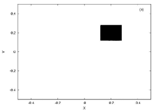
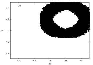
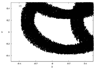
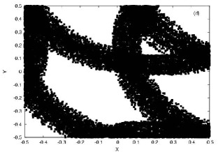
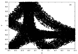
Figure 2: The initial points chosen according to the density in Fig. 1a is shown in Fig. 2a. These are evolved classically using momentum direction ($\varphi$) distributed uniformly in ($0,2\pi$). The distribution of points at time (b) 0.5 (c) 1.0 (d) 1.5 and (e) 2.0 can be compared with the densities in Fig. 1b to 1e respectively.

As a first example, consider a particle in a rectangular box of side $L_{1}=L_{2}=1.0$. Fig. (1a) shows the initial density centred at (0.2,0.2) with $\Delta L=0.15$. The first 5000 quantum Neumann states have been used to expand the initial density. Figs. (1b) to (1e) are the densities at time $t=0.25,0.5,0.75,1.0$ respectively as computed using Eq. (42). For comparison, Fig. 2 is a 2-dimensional view of the density evolved using classical trajectories with their momentum distributed isotropically fnote_momentum . At time $t=0$, the points lie in a square patch as shown in Fig. (2a) while Figs. (2b) to (2e) show the points as they evolve from Fig. (2a) at times $t=0.25,0.5,0.75,1.0$ respectively. Note that the evolution in Fig. 1 reflects isotropy in momentum as expected.

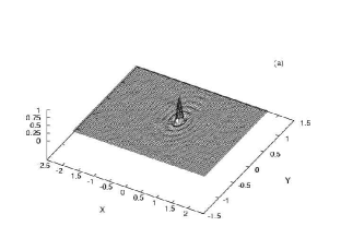
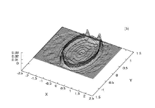
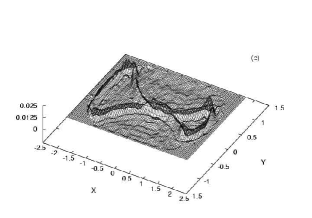
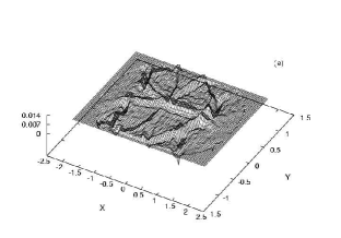
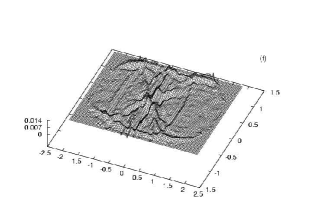
Figure 3: As in Fig. 1 for the stadium billiard at times (a) t=0 (b) t=1 (c) t=2 (d) t=3 (e) t=4 and (f) t=5.

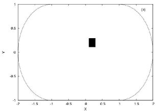
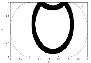
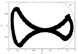
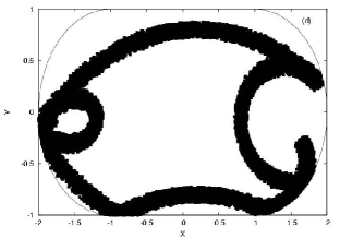
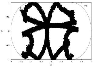
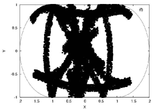
Figure 4: As in Fig. 2 for the stadium billiard at times (a) t=0 (b) t=1 (c) t=2 (d) t=3 (e) t=4 and (f) t=5.

We next consider the chaotic Stadium billiard consisting of two parallel straight segments of length $2$ joined on either end by a semicircle of unit radius. The initial density is again centred at (0.2,0.2) with $\Delta L=0.15$. In this case, the quantum Neumann eigenfunctions have been computed numerically using the boundary integral method. We use the first 1000 eigenfunctions to expand the initial density and evolve it using Eq. (42). Fig. 3 is similar to Fig. 1 but for times t=0,1,2,3,4 and 5 while Fig. 4 (similar to Fig. 2) shows the classical evolution of the initial points at these times. The similarity between the two evolutions is again obvious despite the approximate nature of the eigenfunctions and eigenvalues used.

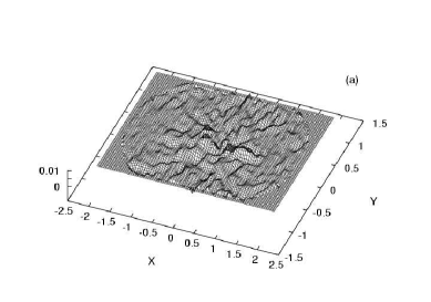
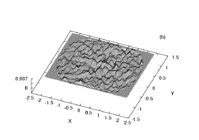
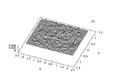
Figure 5: The density evolved using Eq. 42 for the stadium billiard at times (a) t=10 (b) t=20 and (c) t=30.

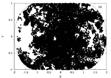
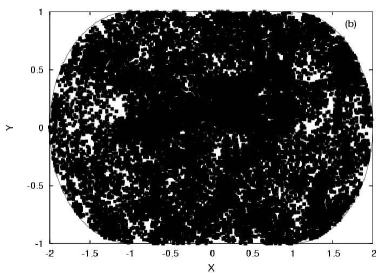
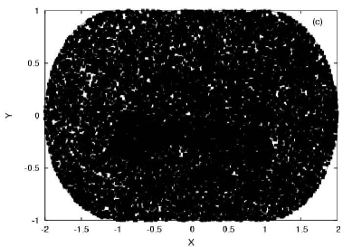
Figure 6: The initial density of Fig. 4a evolved classically using momentum directions distributed uniformly at times (a) t=10 (b) t=20 and (c) t=30.

At longer times, both evolutions lead towards a uniform distribution in ${\bm{q}}$ space. Fig 5 shows the density evolved using Eq. 42 at times t=10, 20 and 30 corresponding on an average to 4.5, 9.0 and 13.6 bounces. This is compared to the classical evolution of the initial points as these times in Fig. 6. Note that the final invariant density should assume a value $\rho\simeq 0.00315$ for the initial density considered. Clearly, the density evolution using Eq. 42 approaches this value with fluctuations around it that diminish with time (see Fig. 5). At $t=30$, the density appears to be nearly uniform in both cases (Fig. (5c) and Fig. (6c)). The decay to the correct (uniform) invariant density is not surprising as the Neumann ground state eigenfunction is uniform and the corresponding eigenvalue $E_{0}=0$ so that $J_{0}(\sqrt{E_{0}}vt)=1$. However, the finer structures are harder to discern at longer times.

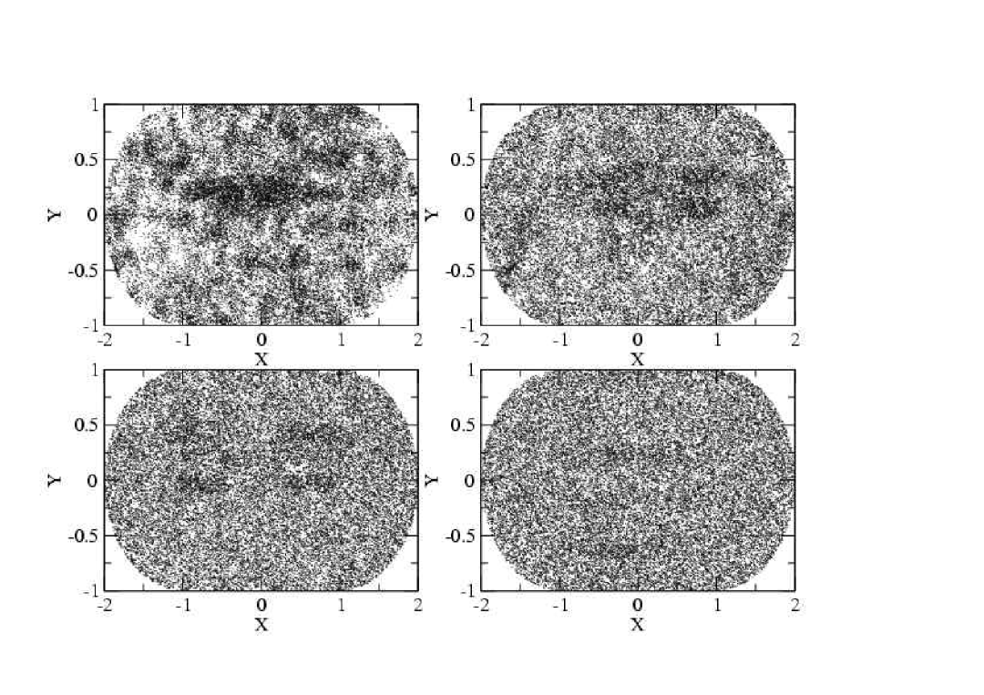
Figure 7: The initial density of Fig. 4a evolved classically using momentum directions distributed uniformly at times t=20 (top-left), t=40 (top-right), t=60 (bottom-left) and (bottom-right) t=110(bottom-right) .

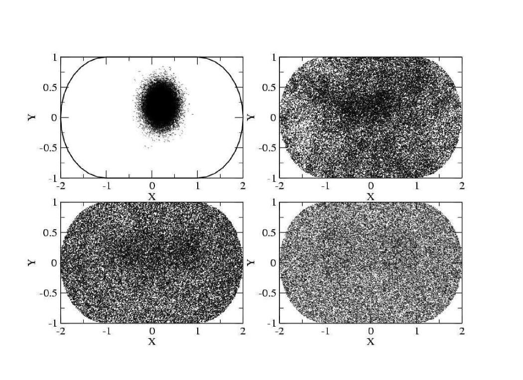
Figure 8: An initial gaussian density (in ${\bm{q}}$ is evolved classically using momentum directions distributed uniformly at times t=0 (top-left), t=20 (top-right), t=40 (bottom-left) and (bottom-right) t=60(bottom-right) .

A closer inspection of the classical evolution however shows that that the density is nonuniform even at t = 30. Fig 7 shows the evolution at t = 20, 40, 60 and 110 using a finer representation (dot size) of a point. In the first two cases, the departure from uniformity seems evident while at t = 60 (average of 27 bounces), a closer inspection shows the presence of four patches of higher density. Finally at t = 110, the density appears to be uniform corresponding to an average of 50 bounces per trajectory. The classical evolution of a Gaussian projected density centred at ${\bm{q}}=(0.2,0.2)$ is shown in Fig. 8 at t = 0, 20, 40 and 60. Note that at t = 40, the density is non-uniform while at t = 60 (average of 27 bounces), the density appears to be uniform. The decay rate thus depends on the initial projected density.

There are two sources of errors in the stadium billiard evolution. In the first place, the quantum Neumann eigenfunctions are approximate classical eigenfunctions, and, the quantum Neumann eigenvalues $\{E_{n}\}$ used in $f(\sqrt{E_{n}}tv)$ are close to but not exactly equal to the classical values. The latter is borne out by the fact that the position of peaks in the fourier transform of $K_{P}$ are close to but not exactly at the quantum Neumann eigenvalues arb2 . The second source of error arises from the the truncation of the basis. As associated problem is the fact that the quantum Neumann eigenfunctions used in the study have been evaluated numerically and hence have errors. In the stadium billiard a thousand eigenstates have been used to expand the initial density while in the rectangle (where an analytic expression is used) five thousand eigenstates have been used to expand and evolve the density. The oscillatory background of the initial density in Fig (3a) is a consequence of truncation error and the error in numerical evaluation of the exact Neumann eigenfunctions. This, coupled with the first source of error mentioned above, can even lead to negative values of the density at some points.

Despite these problems, evolution using the quantum Neumann eigenfunctions and the eigenvalues $\{f(\sqrt{E_{n}}tv)\}$ captures the classical trajectory evolution fairly accurately. The finer structures are reproduced well for about 5 bounces while at longer times, evolution using the quantum Neumann eigenstates leads to the correct invariant density.

V Discussion and Conclusions

We have dealt with the evolution within a billiard enclosure of an initial classical density on the energy shell that is isotropic in momentum. We have constructed an appropriate classical evolution operator (${\cal L}_{P}^{t}$) for the momentum projected density and shown that its approximate (sometimes exact) eigenvalues and eigenfunctions have a one-to-one correspondence with the quantum Neumann eigenvalues and eigenfunctions. Based on this, we have demonstrated that for both the rectangular and stadium billiards, expansion of the initial projected-density using the quantum Neumann eigenfunctions as eigenfunctions of ${\cal L}_{P}^{t}$, captures the classical evolution fairly accurately. While the finer structures are reproduced at shorter times (about 5 bounces for the stadium billiard), evolution using the quantum Neumann eigenstates leads to the correct invariant density at longer times. Note that the spectrum of the evolution operator ${\cal L}_{P}^{t}$ does not fix a time scale in which the initial density decays to the invariant density.

It is instructive to discuss the difference between evolution due to ${\cal L}_{P}^{t}$ and a purely quantum evolution. Specifically, we may ask whether the hat function that we considered as the initial classical density, can be evolved quantum mechanically in an identical fashion at least for short times. The initial quantum state $\psi({\bm{q}},t=0)$ in this case is again a hat function (as it is the square root of the initial density, $\rho({\bm{q}})$ ) and its evolution is governed by

$$\psi({\bm{q}},t)=\sum_{n}c_{n}e^{iE_{n}t}\psi_{n}({\bm{q}},0)$$ (43)

where $c_{n}=\int_{\Delta}\psi_{n}({\bm{q}},0)d{\bm{q}}$. Here $\Delta$ refers to the region in configuration space where the initial wavefunction is non-zero. Eq. 43 however contains no information about the energy or momentum of the underlying classical trajectories. Thus, evolution due to Eq. 43 cannot approximate classical evolution. At the semiclassical level, this is due to the fact that trajectories with all possible energy contribute to the propagator and a correspondence with classical evolution is possible only when the Wigner transform of the initial wavepacket is localized in phase space. In contrast, evolution due to ${\cal L}_{P}^{t}$ has information about the magnitude of the momentum ($v$ in the eigenvalue) and the isotropy in momentum is built into the kernel $K_{P}$ and reflects in the form of the eigenvalue (the Bessel function $J_{0}$).

Another important distinction concerns the decay rates of initial phase space densities that are directionally (or $\varphi$) dependent and independent (isotropic or uniform in $\varphi$). To explore this further, we shall use the operator ${{\cal P}}$ to denote momentum projection. For the anisotropic or directionally dependent initial density $\rho(\bm{q},\bm{p})=\rho(\bm{q},p,\varphi)$,

$$({\cal P}\circ{\cal L}^{t})\rho({\bm{q}},{\bm{p}}) = {\cal P}\sum_{n}C_{n}{\cal L}^{t}\phi_{n}({\bm{q}},{\bm{p}})$$ (44)

$$= \sum_{n}C_{n}e^{\alpha_{n}t}{\cal P}\phi_{n}({\bm{q}},{\bm{p}})$$

$$= \sum_{n}C_{n}e^{\alpha_{n}t}\tilde{\phi}_{n}({\bm{q}}).$$

Here $\tilde{\phi}_{n}({\bm{q}})={\cal P}\phi_{n}({\bm{q}},{\bm{p}})$, $\phi_{n}({\bm{q}},{\bm{p}})$ are the eigenfunctions of ${\cal L}_{P}^{t}$ and the coefficients $C_{n}$ can be determined using the eigenfunctions of ${{\cal L}}^{\dagger}$, the adjoint of ${{\cal L}}$. If the leading $\alpha_{n}$ has a negative real part as in case of hyperbolic systems, the decay to the invariant density is exponential.

In contrast, an isotropic initial density such as $\rho(\bm{q},\bm{p})=\rho(\bm{q},p)=g(\bm{q})\delta(E_{0}-p^{2})$ cannot be expanded in eigenfunctions of ${\cal L}^{t}$. To understand this, note that the only eigenfunction of ${\cal L}^{t}$ which is uniform in $\varphi$ (i.e. isotropic) is the invariant density which is uniform in both ${\bm{q}}$ and $\varphi$. All other densities that are initially uniform in $\varphi$, lose their uniformity (in $\varphi$) as they evolve with ${\cal L}^{t}$. In other words, ${\cal L}^{t}$ does not possess any eigenfunction that is uniform in $\varphi$ but not uniform in $\bm{q}$. Thus $g(\bm{q})\delta(E_{0}-p^{2})$ cannot be expanded in an eigenbasis of ${\cal L}^{t}$. The decay to the invariant density must therefore be dictated by the eigenvalues of ${\cal L}_{P}^{t}$ since

$$({\cal P}{\cal L}^{t})~{}g({\bm{q}})\delta(E_{0}-p^{2})={\cal L}_{P}^{t}~{}\rho_{P}(\bm{q})$$ (45)

where $\rho_{P}({\bm{q}})=\int d\bm{p}~{}\rho(\bm{q},p)=\pi g(\bm{q})$. Thus the decay rates of initial densities that are isotropic must differ from the decay rates of anisotropic densities.

A few conclusions based on the results of the preceding sections are listed below:

• The evolution of a momentum projected density using the (approximate) eigenstates of the momentum projected evolution operator ${\cal L}_{P}^{t}$ captures the classical evolution fairly accurately. The approximate eigenfunctions are the quantum Neumann eigenfunctions while the eigenvalues are related to the quantum Neumann eigenvalues.

• The evolution operator ${\cal L}_{P}^{t}$ is non-multiplicative i.e. ${\cal L}_{P}^{t_{2}+t_{1}}\neq{\cal L}_{P}^{t2}\circ{\cal L}_{P}^{t_{1}}$. Thus, the eigenvalues do not have the form $e^{\lambda_{i}t}$.

• ${\cal L}_{P}^{t}$ preserves positivity of the initial density. However numerical errors and the approximate nature of the eigenvalues and eigenfunctions used in the evolution (Eq. 42) can lead to negative values at some points.

• As the small $t$ behaviour of the density is reproduced by Eq. (42), the correct form of the approximate eigenvalues of ${\cal L}_{P}^{t}$ is $\{J_{0}(\sqrt{E_{n}}vt)\}$ where $E_{n}$ are the quantum Neumann energy eigenvalues. For integrable billiards such as the rectangle, these are the exact eigenvalues.

• For non-polygonal billiards such as the stadium, proof of the existence of a correspondence was indirect, based on the limit of a large number of sides (of the corresponding polygonalized billiard), and, numerical evidence based on a few eigenstates prl2004 ; pramana2005 . The results presented here show that this correspondence must hold for all states as the evolution of the density using the quantum Neumann eigenstates faithfully follows the trajectory picture. This puts the correspondence on a firmer footing.

• The relaxation of an arbitrary projected-density to the uniform, steady-state density can be predicted reasonably using the approximate eigenvalues and eigenfunctions of the projected Perron-Frobenius operator, ${\cal L}_{P}^{t}$.

Appendix A

We shall show here that in polar coordinates ($p,\varphi$),

$$\int{\bm{\delta}}({\bm{p}}-{\bm{p}^{\prime}}^{t})h({\bm{q}^{\prime}},{\bm{p}^{\prime}})d{\bm{p}^{\prime}}=\int d\varphi^{\prime}~{}\delta(\varphi-\varphi^{\prime t})h({\bm{q}^{\prime}},p,\varphi^{\prime}).$$ (46)

where $\varphi^{\prime t}=\varphi^{t}({\bm{q}^{\prime}},p,\varphi^{\prime})$ is the polar angle of the momentum vector ${\bm{p}^{\prime}}$ at time $t$ for an initial phase space point (${\bm{q}^{\prime}},p,\varphi^{\prime}$). Suppressing ${\bm{q}^{\prime}}$, the integral can be expressed as

$$\int\delta(p\cos\varphi-p^{\prime}\cos\varphi^{\prime t})\delta(p\sin\varphi-p^{\prime}\sin\varphi^{\prime t})h({\bm{p}^{\prime}})d{\bm{p}^{\prime}}$$ (47)

where it is assumed that for billiards $p^{\prime t}=p^{\prime}$. Obviously the only value of ${\bm{p}^{\prime}}$ that contributes to the integral is $p^{\prime}=p$ and $\varphi^{\prime t}=\varphi$. In order to carry out the $p^{\prime}$ integration, we may rewrite (47) as

$$\int{\delta(p{\cos\varphi\over\cos\varphi^{\prime t}}-p^{\prime})\over\cos\varphi^{\prime t}}\delta(p\sin\varphi-p^{\prime}\sin\varphi^{\prime t})h({\bm{p}^{\prime}})d{\bm{p}^{\prime}}$$ (48)

On performing the $p^{\prime}$ integration, we have

$$\int d\varphi^{\prime}~{}\delta(p\sin\varphi-p\cos\varphi\tan\varphi^{\prime t}){p\cos\varphi\over\cos^{2}\varphi^{\prime t}}h(p,\varphi^{\prime})$$ (49)

$$= \int d\varphi^{\prime}~{}{\delta(\tan\varphi-\tan\varphi^{\prime t})\over\cos^{2}\varphi^{\prime t}}h(p,\varphi^{\prime})$$

$$= \int d\varphi^{\prime}~{}\delta(\varphi-\varphi^{\prime t})h(p,\varphi^{\prime}).$$

Appendix B Non-multiplicative property of ${\cal L}_{P}^{t}$

The evolution of momentum projected isotropic initial densities on the energy shell is governed by ${\cal L}_{P}^{t}$:

$${\cal L}_{P}^{t}\circ\rho_{P}(\bm{q})=\int d\bm{q}^{\prime}~{}K_{P}(\bm{q},\bm{q}^{\prime},t)~{}\rho_{P}(\bm{q}^{\prime}).$$ (50)

The non-multiplicative property of ${\cal L}_{P}^{t}$ implies

$$\int~{}d{\bm{q}^{\prime\prime}}~{}K_{P}({\bm{q}},{\bm{q}^{\prime\prime}},t_{2})~{}K_{P}({\bm{q}^{\prime\prime}},{\bm{q}^{\prime}},t_{1})\neq K_{P}({\bm{q}},{\bm{q}^{\prime}},t_{1}+t_{2})$$ (51)

This is easiest to visualize when the points ${\bm{q}^{\prime}}$, ${\bm{q}}$ and the times $t_{1}$ and $t_{2}$ are such that such that there is no encounter (reflection) with the boundary of the billiard. As the momentum vector does not change direction, $\varphi^{*}=\varphi$ in Eq. 16. Using Eq. 16 for the projected kernel $K_{P}$,

$$\int d{\bm{q}^{\prime\prime}}~{}K_{P}({\bm{q}},{\bm{q}^{\prime\prime}},t_{2})~{}K_{P}({\bm{q}^{\prime\prime}},{\bm{q}^{\prime}},t_{1})$$ (52)

$$= {1\over(2\pi)^{2}}\int d\varphi d\varphi^{\prime}d{\bm{q}^{\prime\prime}}~{}\delta({\bm{q}}-{\bm{f}_{q}}^{t_{2}}({\bm{q}^{\prime\prime}},p_{0},\varphi^{\prime}))$$

$$~{}~{}~{}~{}~{}~{}~{}~{}~{}\times\delta({\bm{q}^{\prime\prime}}-{\bm{f}_{q}}^{t_{1}}({\bm{q}^{\prime}},p_{0},\varphi))$$

$$= {1\over(2\pi)^{2}}\int d\varphi d\varphi^{\prime}~{}\delta({\bm{q}}-{\bm{f}_{q}}^{t_{2}}({\bm{f}_{q}}^{t_{1}}({\bm{q}^{\prime}},\varphi),\varphi^{\prime}))$$ (53)

$$\neq {1\over 2\pi}\int d\varphi~{}\delta({\bm{q}}-{\bm{f}_{q}^{t_{1}+t_{2}}}({\bm{q}^{\prime}},p_{0},\varphi))$$ (54)

where ${\bm{f}_{q}}$ (also denoted by ${\bm{q}}^{t}$ in the text) is the ${\bm{q}}$-component of the flow $f^{t}$.

The last step can be best understood in terms of Fig. 9 which illustrates the difference in the two time evolutions. The first is a two step evolution from ${\bm{q}^{\prime}}$ to ${\bm{q}^{\prime\prime}}$ in time $t_{1}$ followed by an evolution from ${\bm{q}^{\prime\prime}}$ to ${\bm{q}}$ in time $t_{2}$. These are indicated by solid lines terminated by arrows. The kernel determines the angles $\varphi$ and $\varphi^{\prime}$ which connect ${\bm{q}^{\prime}}$ with ${\bm{q}}$ via the intermediate point ${\bm{q}^{\prime\prime}}$. Depending on the angle $\varphi$, the point ${\bm{q}^{\prime\prime}}$ can lie anywhere on the inner circle ($C_{1}$). Any point ${\bm{q}}$ on the circle $C_{2}$ (with centre on $C_{1}$) has a contribution at time $t_{1}+t_{2}$ from the initial density at ${\bm{q}^{\prime}}$. The second evolution is for a time $t_{1}+t_{2}$ starting from ${\bm{q}^{\prime}}$. The kernel for this evolution contributes when ${\bm{q}}$ lies on the outer circle ($C_{3}$).

Thus, ${\cal L}_{P}^{t_{1}}\circ{\cal L}_{P}^{t_{2}}\neq{\cal L}_{P}^{t_{1}+t_{2}}$. A consequence of the non-multiplicative nature of ${\cal L}_{P}^{t}$ is that its eigenvalues cannot be of the form $e^{\lambda_{i}t}$ i.e. the eigenvalues of ${\cal L}^{t}$ are distinct from the eigenvalues of ${\cal L}_{P}^{t}$ when the initial phase space density is isotropic and constrained to the constant energy surface.

Figure 1: The evolution of a projected-density, $\rho({\bm{q}})$, in the rectangular billiard is computed using the exact quantum Neumann eigenfunctions as the eigenfunctions of the projected Perron-Frobenius operator, ${\cal L}_{P}^{t}$. The initial density is shown in (a) while (b) to (e) show the density at t=0.5, 1.0, 1.5, 2.0 respectively. The evolution reflects isotropy in momentum.

Figure 9: Comparison of two time evolutions in a billiard enclosure (boundary not shown).

References

• (1) P.Β Cvitanovic et al, Chaos: classical and quantum, http://chaosbook.org.
• (2) A.Β Lasota and M.Β MacKey, Chaos, Fractals, and Noise; Stochastic Aspects of Dynamics, Springer-Verlag, Berlin, 1994.
• (3) P.Β Gaspard, Chaos, scattering and statistical Mechanics, Cambridge University Press, 1998.
• (4) J.Β Wilkie and P.Β Brumer, Phys.Β Rev.Β A 55, 29 (1997).
• (5) D.Β Biswas, in Nonlinear Dynamics and Computational Physics, ed. V.Β B.Β Sheorey, Narosa, New Delhi, 1999; chao-dyn/9804013.
• (6) W.Β T.Β Lu, W.Β Zeng and S.Β Sridhar, Phys.Β Rev.Β E 73, 046201 (2006).
• (7) These are not the same as the eigenvalues and eigenfunctions of ${\cal L}^{t}$. See section II and appendix B for non-multiplicative property of ${\cal L}_{P}^{t}$, section III for an illustration using integrable billiards and the discussion in the concluding section.
• (8) D.Β Biswas, Phys.Β Rev.Β Lett. 93, 204102 (2004).
• (9) D.Β Biswas, Pramana - J. Phys, 64, 563 (2005).
• (10) V.Β Milner, J.L.Β Hanssen, W.Β C.Β Campbell and M.Β G.Β Raizen,Phys.Β Rev.Β Lett. 86, 1514 (2001).
• (11) N.Β Friedman, A.Β Kaplan, D.Β Carasso, N.Β Davidson, Phys.Β Rev.Β Lett. 86, 1518 (2001).
• (12) T.Β A.Β Driscoll and H.Β P.Β W.Β Gottlieb, Phys.Β Rev.Β E 68, 016702 (2003); H.-J.Β Stockmann, Quantum Chaos - an Introduction, Cambridge University Press, Cambridge, 1999.
• (13) C.Β Zhang, J.Β Liu, M.Β G.Β Raizen and Q.Β Niu, Phys.Β Rev.Β Lett. 93, 074101 (2004).
• (14) In polygonalized billiards, $\varphi^{\prime t}({\bm{q}}^{\prime},\varphi^{\prime},p)=\varphi^{\prime}$ for a trajectory in the unfolded space which is produced by successive reflections of the billiard domain about the edge that the trajectory strikes. Thus in the unfolded space, a trajectory is a straight line.
• (15) J.Β L.Β Vega, T.Β Uzer and J.Β Ford, Phys.Β Rev.Β E 48, 3414 (1993).
• (16) D.Β Biswas, Phys.Β Rev.Β E 61, 5073 (2000).
• (17) D.Β Biswas, Phys.Β Rev.Β E 63, 016213 (2001).
• (18) D.Β Biswas, Phys.Β Rev.Β E 67, 026208 (2003).
• (19) For a better comparision, for each initial point in ${\bm{q}}$, an isotropic distribution of momentum should be considered.
Refer to caption
Refer to caption
Refer to caption
Refer to caption
Refer to caption