Collection of Mutually Synchronized Chaotic Systems

Abstract

A general explicit coupling for mutual synchronization of two arbitrary identical continuous systems is proposed. The synchronization is proved analytically. The coupling is given for all 19 systems from Sprott’s collection. For one of the systems the numerical results are shown in detail. The method could be adopted for the teaching of the topic.

1 Introduction

Synchronization is a fascinating phenomenon in nature Strogatz (2003); Glass (2001) and a useful one in human activity Nijmeijer (2001). Very simple systems like driven gravitational pendulums or driven nonlinear LCR electric circuits can have chaotic behavior. This means that such systems can not be kept to oscillate in synchrony due to their sensitivity to initial conditions. To synchronize them an additive coupling have been tried that is feasible from the engineering point of view: a constant multiplication of the differences of the states .This type of driving does not work in general. Highly elaborated and mathematically based methods are needed Grosu (1997); Huang (2005); Lerescu et al. (2004). If the above mentioned simple chaotic systems can be synchronized with a precise coupling that is not intuitive at all then the coupling of biological cells that are multivariables nonlinear systems (like millions of neurons that fire together to control our breathing or the coordinated firing of thsousands of pacemakers cells in our hearts Strogatz (2003)) is hard to be imagined. There are known many results on several types of synchronization Pitkovsky et al. (2001). Mutual synchronization is implied in the synchronization of networks Strogatz (2003); Li et al. (2004). Here we give, for the first time, a precise general coupling between two arbitrary identical oscillators in order to get synchronization. The proposed coupling is mathematically based and the synchronization is analytically proved. Numerical results are shown. The paper is organized as follows. In section 2 a coupling is proposed and a theorem is proved for the synchronization of the two systems. Section 3 contains detailed calculations for the Hurwitz matrix and numerical results for one of the systems. The paper ends with conclusions.

2 Mutual Synchronization

Let’s consider two identical nonautonomous systems of the form:

$$\dot{x_{1}}=F(x_{1})+Bu_{1},\qquad y_{1}=Cx_{1},\qquad x_{1}(0)=x_{10}$$ (1)

$$\dot{x_{2}}=F(x_{2})+Bu_{2},\qquad y_{2}=Cx_{2},\qquad x_{2}(0)=x_{20}$$ (2)

where $x_{j}\in\Re^{n}$, $u_{j}\in\Re^{n}$, $j=1,2$. For the prescribed inputs $u_{1}=-\gamma(y_{1}-y_{2})$ and $u_{2}=-\gamma(y_{2}-y_{1})$, the mutual synchronization of (1) and (2) has been studied in Pogromsky (1998) using the powerful concept of passivity Fradkov and Pogromsky (1998). Namely, it is proved that there is a constant $\bar{\gamma}$ such that for $\gamma>\bar{\gamma}$ the systems (1) and (2) synchronize and their dynamics is bounded. Here we consider a particular case with $B=C=\mathbb{I}$ (identity matrix). The inputs $u_{1}$ and $u_{2}$ are not prescribed but they result from the condition of synchronization. In order to avoid the indices with two figures we adopt the notation: $x_{1}=x$, $x_{2}=y$, $u_{1}=S(t)u_{x}(x,y)$ and $u_{2}=S(t)u_{y}(x,y)$. In the following we study the coupled systems:

$$\dot{x}=F(x)+S(t)u_{x}(x,y),\qquad x(0)=x_{0}$$ (3)

$$\dot{y}=F(y)+S(t)u_{y}(x,y),\qquad y(0)=y_{0}$$ (4)

where $S(t)$ is 0 or 1 as a switch. The above systems will synchronize if

$$\lim_{t\rightarrow\infty}\Arrowvert x(t)-y(t)\Arrowvert=0$$

for any $x(0),y(0)\in\mathbb{D}\subset\Re^{n}$. The proposed couplings are:

$$u_{x}(x,y)=\left(H-\frac{\mathrm{d}F(s)}{\mathrm{d}s}\right)\frac{x-y}{2}$$ (5)

$$u_{y}(x,y)=\left(H-\frac{\mathrm{d}F(s)}{\mathrm{d}s}\right)\frac{-x+y}{2}$$ (6)

where $s=\frac{x+y}{2}$ and $H$ is an arbitrary constant Hurwitz matrix (a matrix with negative real part eigenvalues). With equations (3),(4),(5) and (6) we announce the following Theorem.

Theorem.

With $S(t)=1$, the systems (3) and (4) with the coupling (5) and (6) will synchronize for any $x(0)$ and $y(0)$ with $\Arrowvert x(0)-y(0)\Arrowvert$ small enough.

Proof.

Along with $s=\frac{x+y}{2}$ we make the notation $r=\frac{x-y}{2}$. It follows $x=s+r$ and $y=s-r$. Substracting eq. (4) from eq. (3) one has:

$$\dot{r}=\frac{F(s+r)-F(s-r)}{2}+\left(H-\frac{\mathrm{d}F(s)}{\mathrm{d}s}\right)r$$ (7)

We use the Taylor expansions:

$$F(s+r)=F(s)+\frac{\mathrm{d}F(s)}{\mathrm{d}s}r+\frac{1}{2}\frac{\mathrm{d}^{2}F(s)}{\mathrm{d}s_{i}\mathrm{d}s_{j}}r_{i}r_{j}+\ldots$$ (8)

$$F(s-r)=F(s)+\frac{\mathrm{d}F(s)}{\mathrm{d}s}(-r)+\frac{1}{2}\frac{\mathrm{d}^{2}F(s)}{\mathrm{d}s_{i}\mathrm{d}s_{j}}r_{i}r_{j}+\ldots$$ (9)

Using the first three terms in eq. (8) and eq. (9), eq. (7) becomes:

$$\dot{r}=Hr$$ (10)

With $H$ a Hurwitz matrix, eq. (10) assures that $r(t)\rightarrow 0$ for any $r(0)$ for which the Taylor expansions eq. (8) and eq. (9) are valid. This means that $x(t)\rightarrow y(t)$ for any $r(0)=x(0)-y(0)$ with $\Arrowvert x(0)-y(0)\Arrowvert$ small enough. If $F(x)$ is quadratic then the Taylor expansions have only three terms and in this case the eq (10) is not anymore an approximation.

∎

Here we note a significant difference between master-slave synchronization and mutual synchronization. For master-slave synchronization Grosu (1997); Lerescu et al. (2004), the error dynamics is described by an approximate equation like eq (10) for any nonlinear $F(x)$. For mutual synchronization of systems with $F(x)$ a polynomial up to quadratic terms, eq (10) is exact. This could lead to the conclusion that mutual synchronization can be achieved in an easier manner. This is not generally true. A deeper analysis is necessary. In spite of the fact that the eq (10) assures that the two dynamics will be closer and closer, it is not sure that their dynamics are bounded. Even if they are bounded they could have large excursions in the phase space that is very undesirable from the engineering point of view. Further studies are needed to establish how to choose the parameter $p$ (or $p_{1}$,$p_{2}$) in the matrix $H$ (see Table I) and the initial conditions in order to have bounded dynamics of the synchronized systems. Otherwise we can manage this by switching on/off the coupling like this: $S(t)=1$ when $\Arrowvert x-y\Arrowvert<\delta$ and $\Arrowvert x\Arrowvert<R$ where $R$ is the radius of a sphere that contains the attractor of the system $\dot{x}=F(x)$. In Table II (next section), we give the numerical values of the parameter and the initial conditions for which the synchronization was verified numerically.

Matrix $H$ can be chosen in such a manner that the terms from eq. (5) and eq. (6) to be as simple as possible Grosu (1997); Lerescu et al. (2004) and this depends on the particular form of $F(x)$. If $\frac{\mathrm{d}F_{i}(s)}{\mathrm{d}s_{k}}$ is constant then we can choose $H_{ik}=\frac{\mathrm{d}F_{i}(s)}{\mathrm{d}s_{k}}$ and the corresponding term $(u_{x})_{ik}$ will be zero. The simplest coupling in eq. (5) will be when $F(x)$ contains one nonlinear term and this contains one variable. In this case the coupling contains one term (see Table I, below, systems F ,H, I, J, L, M ,N, P, Q, S). We apply this strategy to all systems from Sprott’s collection  Sprott (1994). Table I contains the coupled eq. (5) and eq. (6) for all 19 systems from Sprott’s collection.

Table 1: The coupled systems (1) and (2) of the Sprott’s collection Sprott (1994) with $s_{i}=\frac{x_{i}+y_{i}}{2}$ and $r_{i}=\frac{x_{i}-y_{i}}{2}$ where $i=1,2,3$ and $S(t)=1$.

System	system x	system y	parameter
A	$\par\begin{array}[]{l}\dot{x}_{1}=x_{2}\\ \dot{x}_{2}=-x_{1}+x_{2}x_{3}+(-1-s_{3})r_{2}+(1-s_{2})r_{3}\\ \dot{x}_{3}=1-x_{2}^{2}+pr_{1}+2s_{2}r_{2}\\ \end{array}$	$\par\begin{array}[]{l}\dot{y}_{1}=y_{2}\\ \dot{y}_{2}=-y_{1}+y_{2}y_{3}+(-1-s_{3})(-r_{2})+(1-s_{2})(-r_{3})\\ \dot{y}_{3}=1-y_{2}^{2}+p(-r_{1})+2s_{2}(-r_{2})\\ \end{array}$	$\par\begin{array}[]{l}\\ -1<p<0\\ \\ \end{array}$
B	$\par\begin{array}[]{l}\dot{x}_{1}=x_{2}x_{3}+(1-s_{3})r_{2}+(p_{1}-s_{2})r_{3}\\ \dot{x}_{2}=x_{1}-x_{2}\\ \dot{x}_{3}=1-x_{1}x_{2}+(p_{2}+s_{2})r_{1}+(1+s_{1})r_{2}\\ \end{array}$	$\par\begin{array}[]{l}\dot{y}_{1}=y_{2}y_{3}+(1-s_{3})(-r_{2})+(p_{1}-s_{2})(-r_{3})\\ \dot{y}_{2}=y_{1}-y_{2}\\ \dot{y}_{3}=1-y_{1}y_{2}+(p_{2}+s_{2})(-r_{1})+(1+s_{1})(-r_{2})\\ \end{array}$	$\par\begin{array}[]{l}p_{1}>1\\ p_{2}<-1\\ \\ \end{array}$
C	$\par\begin{array}[]{l}\dot{x}_{1}=x_{2}x_{3}+(p-s_{3})r_{2}-(1+s_{2})r_{3}\\ \dot{x}_{2}=x_{1}-x_{2}\\ \dot{x}_{3}=1-x_{1}^{2}+(1+2s_{1})r_{1}\\ \end{array}$	$\par\begin{array}[]{l}\dot{y}_{1}=y_{2}y_{3}+(p-s_{3})(-r_{2})-(1+s_{2})(-r_{3})\\ \dot{y}_{2}=y_{1}-y_{2}\\ \dot{y}_{3}=1-y_{1}^{2}+(1+2s_{1})(-r_{1})\\ \end{array}$	$\par\begin{array}[]{l}\\ p<0\\ \\ \end{array}$
D	$\par\begin{array}[]{l}\dot{x}_{1}=-x_{2}\\ \dot{x}_{2}=x_{1}+x_{3}\\ \dot{x}_{3}=x_{1}x_{3}+3x_{2}^{2}+(p_{2}-s_{3})r_{1}-\\ \qquad-6s_{2}r_{2}+(p_{1}-s_{1})r_{3}\\ \end{array}$	$\par\begin{array}[]{l}\dot{y}_{1}=-y_{2}\\ \dot{y}_{2}=y_{1}+y_{3}\\ \dot{y}_{3}=y_{1}y_{3}+3y_{2}^{2}+(p_{2}-s_{3})(-r_{1})-\\ \qquad-6s_{2}(-r_{2})+(p_{1}-s_{1})(-r_{3})\\ \end{array}$	$\par\begin{array}[]{l}p_{1}<0\\ p_{1}<p_{2}\\ p_{2}<0\\ \end{array}$
E	$\par\begin{array}[]{l}\dot{x}_{1}=x_{2}x_{3}+(p_{1}-s_{3})r_{2}+(p_{2}-s_{2})r_{3}\\ \dot{x}_{2}=x_{1}^{2}-x_{2}+(1-2s_{1})r_{1}\\ \dot{x}_{3}=1-4x_{1}x_{2}+(-4+4s_{2})r_{1}+4s_{1}r_{2}\\ \end{array}$	$\par\begin{array}[]{l}\dot{y}_{1}=y_{2}y_{3}+(p_{1}-s_{3})(-r_{2})+(p_{2}-s_{2})(-r_{3})\\ \dot{y}_{2}=y_{1}^{2}-y_{2}+(1-2s_{1})(-r_{1})\\ \dot{y}_{3}=1-4y_{1}y_{2}+(-4+4s_{2})(-r_{1})+4s_{1}(-r_{2})\\ \end{array}$	$\par\begin{array}[]{l}p_{1}<0\\ p_{2}>0\\ \\ \end{array}$
F	$\par\begin{array}[]{l}\dot{x}_{1}=x_{2}+x_{3}\\ \dot{x}_{2}=-x_{1}+0.5x_{2}\\ \dot{x}_{3}=x_{1}^{2}-x_{3}+(p-2s_{1})r_{1}\\ \end{array}$	$\par\begin{array}[]{l}\dot{y}_{1}=y_{2}+y_{3}\\ \dot{y}_{2}=-y_{1}+0.5y_{2}\\ \dot{y}_{3}=y_{1}^{2}-y_{3}+(p-2s_{1})(-r_{1})\\ \end{array}$	$\par\begin{array}[]{l}\\ p\in(-2,-0.75)\\ \\ \end{array}$
G	$\par\begin{array}[]{l}\dot{x}_{1}=0.4x_{1}+x_{3}\\ \dot{x}_{2}=x_{1}x_{3}-x_{2}-s_{3}r_{1}+(p-s_{1})r_{3}\\ \dot{x}_{3}=-x_{1}+x_{2}\\ \end{array}$	$\par\begin{array}[]{l}\dot{y}_{1}=0.4y_{1}+y_{3}\\ \dot{y}_{2}=y_{1}y_{3}-y_{2}-s_{3}(-r_{1})+(p-s_{1})(-r_{3})\\ \dot{y}_{3}=-y_{1}+y_{2}\\ \end{array}$	$\par\begin{array}[]{l}\\ p\in(-2.5,-0.6)\\ \\ \end{array}$
H	$\par\begin{array}[]{l}\dot{x}_{1}=-x_{2}+x_{3}^{2}+(p-2s_{3})r_{3}\\ \dot{x}_{2}=x_{1}+0.5x_{2}\\ \dot{x}_{3}=x_{1}-x_{3}\\ \end{array}$	$\par\begin{array}[]{l}\dot{y}_{1}=-y_{2}+y_{3}^{2}+(p-2s_{3})(-r_{3})\\ \dot{y}_{2}=y_{1}+0.5y_{2}\\ \dot{y}_{3}=y_{1}-y_{3}\\ \end{array}$	$\par\begin{array}[]{l}\\ p\in(-2,-0.75)\\ \\ \end{array}$
I	$\par\begin{array}[]{l}\dot{x}_{1}=-0.2x_{2}\\ \dot{x}_{2}=x_{1}+x_{3}\\ \dot{x}_{3}=x_{1}+x_{2}^{2}-x_{3}+(p-2s_{2})r_{2}\\ \end{array}$	$\par\begin{array}[]{l}\dot{y}_{1}=-0.2y_{2}\\ \dot{y}_{2}=x_{1}+y_{3}\\ \dot{y}_{3}=x_{1}+y_{2}^{2}-y_{3}+(p-2s_{2})(-r_{2})\\ \end{array}$	$\par\begin{array}[]{l}\\ p<-0.2\\ \\ \end{array}$
J	$\par\begin{array}[]{l}\dot{x}_{1}=2x_{3}\\ \dot{x}_{2}=-2x_{2}+x_{3}\\ \dot{x}_{3}=-x_{1}+x_{2}+x_{2}^{2}+(p-1-2s_{2})r_{2}\\ \end{array}$	$\par\begin{array}[]{l}\dot{y}_{1}=2y_{3}\\ \dot{y}_{2}=-2y_{2}+y_{3}\\ \dot{y}_{3}=-y_{1}+y_{2}+y_{2}^{2}+(p-1-2s_{2})(-r_{2})\\ \end{array}$	$\par\begin{array}[]{l}\\ p<0\\ \\ \end{array}$
K	$\par\begin{array}[]{l}\dot{x}_{1}=x_{1}x_{2}-x_{3}-s_{2}r_{1}+(p-s_{1})r_{2}\\ \dot{x}_{2}=x_{1}-x_{2}\\ \dot{x}_{3}=x_{1}+0.3x_{3}\\ \end{array}$	$\par\begin{array}[]{l}\dot{y}_{1}=y_{1}y_{2}-y_{3}-s_{2}(-r_{1})+(p-s_{1})(-r_{2})\\ \dot{y}_{2}=y_{1}-y_{2}\\ \dot{y}_{3}=y_{1}+0.3y_{3}\\ \end{array}$	$\par\begin{array}[]{l}\\ p\in(-3.3,-0.51)\\ \\ \end{array}$
L	$\par\begin{array}[]{l}\dot{x}_{1}=x_{2}+3.9x_{3}\\ \dot{x}_{2}=0.9x_{1}^{2}-x_{2}+(p-1.8s_{1})r_{1}\\ \dot{x}_{3}=1-x_{1}\\ \end{array}$	$\par\begin{array}[]{l}\dot{y}_{1}=y_{2}+3.9y_{3}\\ \dot{y}_{2}=0.9y_{1}^{2}-y_{2}+(p-1.8s_{1})(-r_{1})\\ \dot{y}_{3}=1-y_{1}\\ \end{array}$	$\par\begin{array}[]{l}\\ p<0\\ \\ \end{array}$
M	$\par\begin{array}[]{l}\dot{x}_{1}=-x_{3}\\ \dot{x}_{2}=-x_{1}^{2}-x_{2}+(p+2s_{1})r_{1}\\ \dot{x}_{3}=1.7+1.7x_{1}+x_{2}\\ \end{array}$	$\par\begin{array}[]{l}\dot{y}_{1}=-y_{3}\\ \dot{y}_{2}=-y_{1}^{2}-y_{2}+(p+2s_{1})(-r_{1})\\ \dot{y}_{3}=1.7+1.7y_{1}+y_{2}\\ \end{array}$	$\par\begin{array}[]{l}\\ p\in(-1.7,0)\\ \\ \end{array}$
N	$\par\begin{array}[]{l}\dot{x}_{1}=-2x_{2}\\ \dot{x}_{2}=x_{1}+x_{3}^{2}+(p-2s_{3})r_{3}\\ \dot{x}_{3}=1+x_{2}-2x_{3}\\ \end{array}$	$\par\begin{array}[]{l}\dot{y}_{1}=-2y_{2}\\ \dot{y}_{2}=y_{1}+y_{3}^{2}+(p-2s_{3})(-r_{3})\\ \dot{y}_{3}=1+y_{2}-2y_{3}\\ \end{array}$	$\par\begin{array}[]{l}\\ p<0\\ \\ \end{array}$
O	$\par\begin{array}[]{l}\dot{x}_{1}=x_{2}\\ \dot{x}_{2}=x_{1}-x_{3}\\ \dot{x}_{3}=x_{1}+x_{1}x_{3}+2.7x_{2}-s_{3}r_{1}+(p-s_{1})r_{3}\\ \end{array}$	$\par\begin{array}[]{l}\dot{y}_{1}=y_{2}\\ \dot{y}_{2}=y_{1}-y_{3}\\ \dot{y}_{3}=y_{1}+y_{1}y_{3}+2.7y_{2}-s_{3}(-r_{1})+(p-s_{1})(-r_{3})\\ \end{array}$	$\par\begin{array}[]{l}\\ p\in(-1,-0.37)\\ \\ \end{array}$
P	$\par\begin{array}[]{l}\dot{x}_{1}=2.7x_{2}+x_{3}\\ \dot{x}_{2}=-x_{1}+x_{2}^{2}+(p-2s_{2})r_{2}\\ \dot{x}_{3}=x_{1}+x_{2}\\ \end{array}$	$\par\begin{array}[]{l}\dot{y}_{1}=2.7y_{2}+y_{3}\\ \dot{y}_{2}=-y_{1}+y_{2}^{2}+(p-2s_{2})(-r_{2})\\ \dot{y}_{3}=y_{1}+y_{2}\\ \end{array}$	$\par\begin{array}[]{l}\\ p\in(-1,\frac{10}{27})\\ \\ \end{array}$
Q	$\par\begin{array}[]{l}\dot{x}_{1}=-x_{3}\\ \dot{x}_{2}=x_{1}-x_{2}\\ \dot{x}_{3}=3.1x_{1}+x_{2}^{2}+0.5x_{3}+(p-2s_{2})r_{2}\\ \end{array}$	$\par\begin{array}[]{l}\dot{y}_{1}=-y_{3}\\ \dot{y}_{2}=y_{1}-y_{2}\\ \dot{y}_{3}=3.1y_{1}+y_{2}^{2}+0.5y_{3}+(p-2s_{2})(-r_{2})\\ \end{array}$	$\par\begin{array}[]{l}\\ p\in(-3.1,-1.8)\\ \\ \end{array}$
R	$\par\begin{array}[]{l}\dot{x}_{1}=0.9-x_{2}\\ \dot{x}_{2}=0.4+x_{3}\\ \dot{x}_{3}=x_{1}x_{2}-x_{3}+(1-s_{2})r_{1}+(p-s_{1})r_{2}\\ \end{array}$	$\par\begin{array}[]{l}\dot{y}_{1}=0.9-y_{2}\\ \dot{y}_{2}=0.4+y_{3}\\ \dot{y}_{3}=y_{1}y_{2}-y_{3}+(1-s_{2})(-r_{1})+(p-s_{1})(-r_{2})\\ \end{array}$	$\par\begin{array}[]{l}\\ p<-1\\ \\ \end{array}$
S	$\par\begin{array}[]{l}\dot{x}_{1}=-x_{1}-4x_{2}\\ \dot{x}_{2}=x_{1}+x_{3}^{2}+(p-2s_{3})r_{3}\\ \dot{x}_{3}=1+x_{1}\\ \end{array}$	$\par\begin{array}[]{l}\dot{y}_{1}=-y_{1}-4y_{2}\\ \dot{y}_{2}=y_{1}+y_{3}^{2}+(p-2s_{3})(-r_{3})\\ \dot{y}_{3}=1+y_{1}\\ \end{array}$	$\par\begin{array}[]{l}\\ p\in(0,1)\\ \\ \end{array}$

3 Numerical results

We give detailed calculations for the system S from the Sprott’s collection (see Table I). The system in $x$ is:

$$\begin{array}[]{lcl}\dot{x}_{1}&=&-x_{1}+4x_{2}\\ \dot{x}_{2}&=&x_{1}+x_{3}^{2}\\ \dot{x}_{3}&=&1+x_{1}\end{array}$$ (11)

The Jacobian is:

$$\frac{\mathrm{d}F(s)}{\mathrm{d}s}=\left(\begin{array}[]{ccc}-1&-4&0\\ 1&0&2s_{3}\\ 1&0&0\\ \end{array}\right)$$ (12)

We can choose matrix $H$ as:

$$H=\left(\begin{array}[]{ccc}-1&-4&0\\ 1&0&p\\ 1&0&0\\ \end{array}\right)$$ (13)

The characteristic equation is:

$$\lambda^{3}+a_{1}\lambda^{2}+a_{2}\lambda+a_{3}=0$$ (14)

where

$$a_{1}=1,\quad a_{2}=4,\quad a_{3}=4p.$$ (15)

The Ruth-Hurwitz conditions (for eq. (14)) are:

$$a_{1}>0,a_{1}a_{2}-a_{3}>0,a_{3}>0.$$ (16)

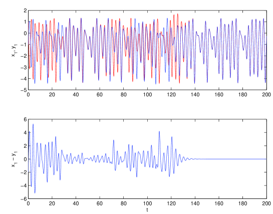
Figure 1: Numerical results. $S(t)=0$ for $t<120$ and $S(t)=1$ for $t>120$ for the coupled systems (3) and (3). Initial conditions are $x_{1}(0)=x_{2}(0)=x_{3}(0)=-1$ and $y_{1}(0)=y_{2}(0)=y_{3}(0)=1$. Top figure represents $x_{1}$ and $y_{1}$ and the bottom figure is the error function $x_{1}-y_{1}$. It takes about 15 time units since the mutual coupling is switched on (at $t=120$) until the synchronization is achieved.

This gives for the parameter $p$ the condition $0<p<1$. In this case we have:

$$\begin{array}[]{ll}u_{x}^{1}=0&u_{y}^{1}=0\\ u_{x}^{2}=(p-2s_{3})r_{3}&u_{y}^{2}=(p-2s_{3})(-r_{3})\\ u_{x}^{3}=0&u_{y}^{3}=0\\ \end{array}$$ (20)

The two coupled systems follow now as (see Figure 1 for numerical simulation):

$$\dot{x_{1}} = -x_{1}+4x_{2}$$

$$\dot{x_{2}} = x_{1}+4x_{3}^{2}+S(t)(p-2s_{3})r_{3}$$ (21)

$$\dot{x_{3}} = 1+x_{1}$$

$$\dot{y_{1}} = -y_{1}+4y_{2}$$

$$\dot{y_{2}} = y_{1}+4y_{3}^{2}+S(t)(p-2s_{3})(-r_{3})$$ (22)

$$\dot{y_{3}} = 1+y_{1}$$

where $s_{3}=\frac{x_{3}+y_{3}}{2}$ and $r_{3}=\frac{x_{3}-y_{3}}{2}$.

In the same manner can be written the couplings for all 19 systems from Sprott’s collection. If the conditions (16) can not be fulfilled with one parameter $p$ then a second parameter should be introduced (see Table I, systems B, C, D, E, O, R). The Hurwitz matrix should be chosen the same as in Lerescu et al. (2004). The choice of $H$ is not unique for systems that have several terms in the coupling term. And, as was mentioned in the previous section, the theorem does not assures that the dynamics of the coupled systems is bounded.

In Table II we present numerical values for the parameter $p$ or $p_{1},p_{2}$ (see Table I) and initial conditions for which the synchronization was verified numerically. It can be observed that it was not difficult to find such numerical values. They are rather homogeneous. When the dynamics was far from the dynamics of the original system $\dot{x}=F(x)$ for $x(0)=-y(0)=(1,1,1)$ then we changed to the initial conditions $x(0)=-y(0)=(0.1,0.1,0.1)$. Further studies are needed to find analytic conditions for the matrix Hurwitz H and the initial conditions that assure a bounded dynamics for the coupled system.

Table 2: Numerical values of the parameter $p$ or $p_{1},p_{2}$ and initial conditions for the systems in Table I for which the synchronization was verified numerically.

System	A	B	C	D	E	F	G	H	I	J	K	L	M	N	O	P	Q	R	S
$\begin{array}[]{c}x_{i}(0)=-y_{i}(0)\\ i=1,2,3\\ \end{array}$	1	1	1	0.1	1	0.1	0.1	1	1	1	1	1	0.1	1	0.1	0.1	1	1	1
p	-0.1		-1			-1	-1	-1	-10	-1	-1	-1	-1	-1	-0.5	-0.5	-2	-2	0.5
$\begin{array}[]{c}p_{1}\\ p_{2}\\ \end{array}$		$\begin{array}[]{c}2\\ -2\\ \end{array}$		$\begin{array}[]{c}-0.1\\ -0.05\\ \end{array}$	$\begin{array}[]{c}-1\\ 1\\ \end{array}$

Using the same notation like the Table I and the Hurwitz matrix found in Lerescu et al. (2004), two Lorenz systems mutually synchronized look like:

$$\dot{x}_{1} = s(-x_{1}+x_{2})$$

$$\dot{x}_{2} = rx_{1}-x_{2}-x_{1}x_{3}+S(t)(s_{1}x_{3}+(p+s_{3})r_{1})$$ (23)

$$\dot{x}_{3} = -bx_{3}+x_{1}x_{2}-S(t)(s_{1}r_{2}+s_{2}r_{1})$$

$$\dot{y}_{1} = s(-y_{1}+y_{2})$$

$$\dot{y}_{2} = ry_{1}-y_{2}-y_{1}y_{3}+S(t)(-s_{1}y_{3}+(p+s_{3})(-r_{1}))$$ (24)

$$\dot{y}_{3} = -by_{3}+y_{1}y_{2}+S(t)(s_{1}r_{2}+s_{2}r_{1})$$

For (s,r,b,p) = (16, 45.6, 4, -60) and $x(0)=-y(0)=(1,1,1)$, the synchronization was verified numerically. In Pogromsky (1998), the mutual synchronization of two Lorenz systems was obtained by using one term in the first equations and any intial conditions.

Also for the simplest chaotic sytems $\dddot{x}+a\ddot{x}-\dot{x}^{2}+x=0$, the coupled systems that will synchronize look like: $\dddot{x}+a\ddot{x}-\dot{x}^{2}+x+(p+(\dot{x}+\dot{y}))(\dot{x}-\dot{y})=0$ and $\dddot{y}+a\ddot{y}-\dot{y}^{2}+y+(p+(\dot{x}+\dot{y}))(-\dot{x}+\dot{y})=0$ and for $(a,p)=(2,-1)$ and $(x(0),\dot{x}(0),\ddot{x}(0))=-(y(0),\dot{y}(0),\ddot{y}(0))=(1,1,1)$ the synchronization was checked numerically.

4 Conclusions

A precise analytical scheme for mutual synchronization is proposed. The method is mathematical rigorous in terms of choosing the expression of coupling and indications are given how to avoid unbounded dynamics of the coupled systems.

References

• Strogatz (2003) S. Strogatz, Synch: the emerging science of spontaneous order (Hyperion, 2003).
• Glass (2001) L. Glass, Nature 410, 277 (2001).
• Nijmeijer (2001) H. Nijmeijer, Physica D 154, 219 (2001).
• Grosu (1997) I. Grosu, Phys. Rev. E 56, 3709 (1997).
• Huang (2005) D. Huang, Phys. Rev. E 71, 037203 (2005).
• Lerescu et al. (2004) A. Lerescu, N. Constandache, S. Oancea, and I. Grosu, Chaos, Solitons and Fractals 22, 599 (2004).
• Pitkovsky et al. (2001) A. Pitkovsky, M. Rosenblum, and R. Kurths, Synchronization: an universal concept in nonlinear science (Cambridge University Press, 2001).
• Li et al. (2004) X. Li, X. Wang, and G. Chen, IEEE Tr CAS I 51, 2074 (2004).
• Pogromsky (1998) A. Pogromsky, Int. J. of Bif and Chaos 8, 295 (1998).
• Fradkov and Pogromsky (1998) A. Fradkov and A. Pogromsky, Introduction to Control of Oscillations and Chaos (World Scientific, 1998).
• Sprott (1994) J. Sprott, Phys. Rev. E 55, 5285 (1994).