PACS numbers : 47.20.Ky, 42.81.Dp, 02.30.Jr

Key words : General fifth-order nonlinear evolution equation; Lagrangian representation; Integrable hierarchy; Lax representation and bi-Hamiltonian structure; soliton solution.

A general form of the fifth-order nonlinear evolution equation is considered. Helmholtz solution of the inverse variational problem is used to derive conditions under which this equation admits an analytic representation. A Lennard type recursion operator is then employed to construct a hierarchy of Lagrangian equations. It is explicitly demonstrated that the constructed system of equations has a Lax representation and two compatible Hamiltonian structures. The homogeneous balance method is used to derive analytic soliton solutions of the third- and fifth-order equations.

I. Introduction In recent years studies in fifth-order nonlinear evolution equations have received considerable attention primarily because these equations possess a host of connections with other integrable equations which play a role in diverse areas of physics ranging from nonlinear optics [1] to Bose-Einstein condensation [2]. For example, Özer and Döken [3] used a multiple-scale method to derive the fifth-order Korteweg-de Vries (KdV) equation from the higher-order nonlinear Schödinger equation. On the other hand, a similar method could also be used [4] to obtain the nonlinear Schödinger equation from fifth-order KdV flow [5], Sawada-Kotera equation [6] and Kaup-Kupershmidt equation [7].

Third-order evolution equations can often be solved either by the use of an inverse spectral method or by taking recourse to a simple change of variables. This is true for both the linearly dispersive KdV equation and the nonlinearly dispersive Rosenau-Hymann equation [8]. In contrast, it is quite difficult to obtain solutions of the fifth-order equations. This might be another point of interest for recent studies [9] in these equations.

In this work we derive the condition under which the general fifth-order nonlinear evolution equation

$$u_{t}=u_{5x}+Auu_{3x}+Bu_{x}u_{2x}+Cu^{2}u_{x},\,\,\,u=x(x,t)$$ (1)

admits an analytic representation [10] or follows from a Lagrangian. Here $A$, $B$ and $C$ are constant model parameters. The subscripts on $u$ denote partial derivatives with respect to that variable and, in particular, $u_{nx}=\frac{\partial^{n}u}{\partial x^{n}}$. We use the fifth-order Lagrangian equation to define an integrable hierarchy. Further, we provide a Lax representation [5] and construct a bi-Hamiltonian structure [11] for the system. The Lagrangian approach to nonlinear evolution equation has two novel features. First, from the Lagrangians or Lagrangian densities we can construct Hamiltonian densities [12] which form the set of involutive conserved densities of the system. Second, the expression for the Lagrangian represents a useful basis to construct an approximate solution for the evolution equation [13,14]. We shall, however, use a direct method [15] to obtain explicit analytic soliton solutions.

In Sec.II we deal with the inverse variational problem for $(1)$ and derive relations between the model parameters for the equation to be Lagrangian. We then make use of an appropriate pseudo-differential operator to construct a hierarchy of equations and present results for the first few members of the hierarchy. In Sec.III we find their Lax representations and examine the bi-Hamiltonian structure. The results presented are expected to serve as a useful test of integrability. We devote Sec.IV to present explicit solitonic solutions by using the homogeneous balance method (HB). We present some concluding remarks in Sec.V. II. Lagrangian system of equations

In the calculus of variation one is concerned with two types of problems, namely, the direct and the inverse problem of Newtonian mechanics. The direct problem is essentially the conventional one in which one first assigns a Lagrangian and then computes the equations of motion through Lagrange’s equations. As opposed to this, the inverse problems begins with the equation of motion and then constructs a Lagrangian consistent with the variational principle [10]. The inverse problem of the calculus of variation was solved by Helmholtz [16] during the end of the nineteenth century. For continuum mechanics the Helmholtz version of the inverse problem proceeds by considering an r-tuple of differentiable functions written as

$$P[v]=P(x,v^{(n)})\,\,\epsilon\,\,{\cal A}^{r}$$ (2)

and then defining the so-called Fréchet derivative. The Fréchet derivative of P is the differential operator $D_{P}:\,\,{\cal A}^{q}\rightarrow{\cal A}^{r}$ and is given by

$$D_{P}(Q)={\frac{d}{d\epsilon}}\vline_{{}_{{}_{{}_{{}_{\epsilon=0}}}}}P[v+\,\epsilon\,Q[v]]$$ (3)

for any $Q\,\,\epsilon\,\,{\cal A}^{q}$. The Helmholtz condition asserts that P is the Euler-Lagrange expression for some variational problem iff $D_{P}$ is self-adjoint. When self-adjointness is guaranteed, a Lagrangian density for P can be explicitly constructed using the homotopy formula

$${\cal L}[v]=\int_{0}^{1}vP[\lambda v]d\lambda\,\,.$$ (4)

In the following we shall demand the Helmholtz condition to be valid for (1). This will provide us with certain constraints between the model parameters of (1) to follow from a Lagrangian density.

A single evolution equation $u_{t}=P[u]$, $u\,\,\epsilon\,\,\mathbb{R}$ is never the Euler-Lagrange equation of a variational problem [16]. One common trick to put a single evolution equation into a variational form is to replace $u$ by a potential function

$$u=-w_{x},\,\,w=w(x,t)\,\,.$$ (5)

The function $w$ is often called the Casimir potential. In terms of the Casimir potential, (1) reads

$$w_{xt}=P[w_{x}]\,\,,$$ (6)

where

$$P[w_{x}]=w_{6x}-Aw_{x}w_{4x}-Bw_{2x}w_{3x}+C{w_{x}}^{2}w_{2x}\,\,.$$ (7)

From (3) and (7) we obtain

$$D_{P}=D_{6x}-Aw_{x}D_{4x}-Aw_{4x}D_{x}-Bw_{2x}D_{3x}-Bw_{3x}D_{2x}$$

$$+C{w_{x}}^{2}D_{2x}+2Cw_{x}w_{2x}D_{x}\,\,.$$ (8)

To construct the adjoint operator $D_{p}^{*}$ of the above Fréchet derivative we rewrite (8) as

$$D_{P}=\sum_{j}P_{j}[w_{x}]D_{j}$$ (9)

and make use of the definition [16]

$$D^{*}_{P}=\sum(-D)_{j}.P_{j}$$ (10)

meaning that for any $Q\,\,\epsilon\,\,\cal A$

$$D^{*}_{P}Q=\sum_{j}(-D)_{j}[P_{j}Q]\,\,.$$ (11)

This gives

$$D^{*}_{P}=D_{6x}-Aw_{x}D_{4x}-(3A-B)w_{4x}D_{x}-(4A-B)w_{2x}D_{3x}$$

$$-(6A-2B)w_{3x}D_{2x}+Cw_{x}^{2}D_{2x}+2Cw_{x}w_{2x}D_{x}\,\,.$$ (12)

Demanding variational self-adjointness we obtain from (8) and (12)

$$B=2A$$ (13)

while $C$ remains unrestricted. Thus the nonlinear equation

$$u_{t}=u_{5x}+Auu_{3x}+2Au_{x}u_{2x}+Cu^{2}u_{x}$$ (14)

forms a Lagrangian system. We note that the Lax equation [5] with $A=10$, $B=20$ and $C=30$ and the Ito equation [17] with $A=3$, $B=6$ and $C=2$ are of the form (14) while the Sawada-Kotera equation with $A=B=C=5$ and the Kaup-Kupershmidt equation with $A=10$, $B=25$ and $C=20$ are non-Lagrangian.

We now use the fifth-order Lagrangian equation (14) to define an integrable hierarchy. To that end we introduce a pseudo-differential or integro-differential operator $\Lambda$ which acts on a generic function $f(x)$ to give [18]

$$\Lambda f(x)=f_{xx}-puf(x)+qu_{x}\int_{x}^{+\infty}dyf(y).$$ (15)

Further, we introduce a function $g_{x}^{(n)}$ to follow from

$${\Lambda}^{n}u_{x}(x,t)=g_{x}^{(n)},n=0,1,2....\,\,\,\,.$$ (16)

Here $g_{x}^{(n)}$ is a polynomial in $u$ and its $x$-derivatives (up to derivative of order 2n). Using $f(x)=u_{x}(x,t)$ in (15) we have

$$\Lambda f(x)=(u_{2x}-\frac{p+q}{2}u^{2})_{x}\,\,.$$ (17)

From (16) and (17)

$${\Lambda}^{2}u_{x}(x,t)=u_{5x}-(2p+q)uu_{3x}-(3p+4q)u_{x}u_{2x}+(p+q)(p+\frac{q}{2})u^{2}u_{x}\,\,.$$ (18)

Comparing (14) and (18) and identifying ${\Lambda}^{2}u_{x}(x,t)$ as $u_{t}$ we can express $p$ and $q$ in terms of $A$. This allows us to write

$$C=(p+q)(p+\frac{q}{2})=\frac{3A^{2}}{10}\,\,.$$ (19)

Therefore, the general form of the fifth-order Lagrangian equation generated by $\Lambda$ via (16) has the form

$$u_{t}=u_{5x}+Auu_{3x}+2Au_{x}u_{2x}+\frac{3A^{2}}{10}u^{2}u_{x}\,\,.$$ (20)

We have used (16) to generate a hierarchy of nonlinear evolution equations for $n=0,1,2,3$ etc. The first member of the hierarchy ($n=0$) is a linear equation given by

$$u_{t}=u_{x}\,\,,$$ (21)

while the second one ($n=1$) is a third-order nonlinear equation

$$u_{t}=u_{3x}+\frac{3A}{5}uu_{x}\,\,.$$ (22)

The third member ($n=2$) is obviously the fifth-order equation given in (20). The corresponding seventh and ninth order equations are given by

$$u_{t}=u_{7x}+\frac{7A}{5}u_{5x}u+\frac{21A}{5}u_{4x}u_{x}+7Au_{3x}u_{2x}+\frac{7A^{2}}{10}u^{2}u_{3x}$$

$$+\frac{14A^{2}}{5}uu_{x}u_{2x}+\frac{7A^{2}}{10}{u_{x}}^{3}+\frac{7A^{3}}{50}u^{3}u_{x}$$ (23)

and

$$u_{t}=u_{9x}+\frac{9A}{5}u_{7x}u+\frac{36A}{5}u_{6x}u_{x}+\frac{84A}{5}u_{5x}u_{2x}+\frac{126A}{5}u_{4x}u_{3x}+\frac{651A^{2}}{50}u_{x}u_{2x}^{2}$$

$$+\frac{483A^{2}}{50}u_{x}^{2}u_{3x}+\frac{63A^{2}}{5}uu_{2x}u_{3x}+\frac{378A^{2}}{50}uu_{x}u_{4x}+\frac{63A^{2}}{50}u^{2}u_{5x}$$

$$+\frac{63A^{3}}{50}uu_{x}^{3}+\frac{126A^{3}}{50}u^{2}u_{x}u_{2x}+\frac{21A^{3}}{50}u^{3}u_{3x}+\frac{63A^{4}}{1000}u^{4}u_{x}.$$ (24)

III. Lax representation and bi-Hamiltonian structure

Integrable nonlinear evolution equations admit zero curvature or Lax representation [5]. These equations are characterized by an infinite number of conserved densities which are in involution. Moreover, each number of the hierarchy has a bi-Hamiltonian structure [11].In the following we demonstrate these three important features for our equations in (20)-(24).

The Lax representation of nonlinear evolution equations is based on the algebra of differential operators. Here one considers two linear operators $L$ and $M$ . The eigenvalue equation for the operator $L$ is given by

$$L\psi=\lambda\psi$$ (25)

with $\psi$, the eigenfunction and $\lambda$, the corresponding eigenvalue. The operator $M$ characterizes the change of eigenfunctions with the parameter $t$ which, in a nonlinear evolution equation, usually corresponds to the time . The general form of this equation is

$${\psi}_{t}=M\psi\,\,.$$ (26)

If we now invoke a basic result of the inverse spectral method that $\frac{d\lambda}{dt}=0$ for non-zero eigenfunctions [19], then (25) and (26) will immediately give

$$\frac{\partial L}{\partial t}=[M,L]\,\,.$$ (27)

Equation (27) is called the Lax equation and $L$ and $M$ are called the Lax pairs. In the context of Lax’s method it is often said that $L$ defines the original spectral problem while $M$ represents an auxiliary spectral problem. For a given nonlinear evolution equation one needs to find these operators. This is not always a straightforward task. In fact, no systematic procedure has been derived to determine whether a nonlinear partial differential equation can be represented in the form (27).

We shall now find the Lax representation for the hierarchy of equations given in (20)-(24). We first note that as one goes along the hierarchy the original spectral problem remains invariant while the auxiliary spectral problem goes on changing. Keeping this in mind we take

$$\!\!\!\!\!\!\!\!\!\!\!\!\!\!\!\!\!\!\!\!\!\!\!\!\!\!\!\!\!\!\!\!\!\!\!\!\!\!\!\!\!\!\!\!\!\!\!\!\!\!\!\!\!\!\!\!L=\partial_{x}^{2}+\frac{A}{10}u$$ (28)

In writing (28) we have exploited the similarity between (22) and the KdV equation. As regards the auxiliary spectral problem we postulate that for an evolution equation of the form $u_{t}=K[u]$ the terms in the Fréchet derivative of $K[u]$ contribute additively with unequal weights to form the operator $M$ such that $L$ and $M$ via (22) reproduces $K[u]$ . Of course, there should not be any inconsistency in determining the values of the weight factors. For (22) the Fréchet derivative of $K[u]$ can be obtained as

$$D_{P}=\partial_{x}^{3}+\frac{3A}{5}(u\partial_{x}+u_{x})\,\,.$$ (29)

We shall, therefore, write

$$M_{3}=a\partial_{x}^{3}+\frac{3A}{5}(bu\partial_{x}+cu_{x})\,\,.$$ (30)

Here the subscript $3$ on $M$ indicates that (30) represents the second Lax operator for the third-order equation. We shall follow this convention throughout. Equations (22), (27), (28) and (30) can be combined to get $a=4$, $b=1$ and $c=\frac{1}{2}$. Thus we have

$$\!\!\!\!\!\!\!\!\!\!\!\!\!\!\!\!\!\!\!\!\!\!\!\!\!\!\!\!\!\!\!\!\!\!\!\!\!\!\!\!\!\!\!\!\!\!\!\!\!\!\!\!\!\!\!\!\!\!\!\!\!\!\!\!\!\!\!\!\!\!\!\!\!\!\!\!\!\!\!\!\!\!\!\!\!\!\!\!\!\!\!\!\!\!\!\!\!\!\!\!\!\!\!\!\!\!\!\!\!\!\!\!M_{3}=4\partial_{x}^{3}+\frac{3A}{5}(u\partial_{x}+\frac{1}{2}u_{x})\,\,.$$ (31)

Similarly, we find the results

$$M_{5}=16\partial_{x}^{5}+4Au\partial_{x}^{3}+6Au_{x}\partial_{x}^{2}+5Au_{2x}\partial_{x}+\frac{3A^{2}}{10}u^{2}\partial_{x}+\frac{3A}{2}u_{3x}+\frac{3A^{2}}{10}uu_{x}\,\,,$$ (32)

$$M_{7}=64\partial_{x}^{7}+\frac{112A}{5}u\partial_{x}^{5}+56Au_{x}\partial_{x}^{4}+84Au_{2x}\partial_{x}^{3}+\frac{14A^{2}}{5}u^{2}\partial_{x}^{3}+70Au_{3x}\partial_{x}^{2}$$

$$+\frac{42A^{2}}{5}uu_{x}\partial_{x}^{2}+\frac{161A}{5}u_{4x}\partial_{x}+7A^{2}uu_{2x}\partial_{x}+\frac{147A^{2}}{30}u_{x}^{2}\partial_{x}+\frac{7A^{3}}{50}u^{3}\partial_{x}$$

$$+\frac{63A}{10}u_{5x}+\frac{21A^{2}}{10}uu_{3x}+\frac{21A^{2}}{5}u_{x}u_{2x}+\frac{21A^{3}}{100}u^{2}u_{x}\,\,,$$ (33)

and

$$M_{9}=256\partial_{x}^{9}+\frac{576A}{5}u\partial_{x}^{7}+\frac{51A}{2}u_{7x}+\frac{2016A}{5}u_{x}\partial_{x}^{6}+\frac{897A}{5}u_{6x}\partial_{x}+\frac{4368A}{5}u_{2x}\partial_{x}^{5}$$

$$+\frac{2814A}{5}u_{5x}\partial_{x}^{2}+1176Au_{3x}\partial_{x}^{4}+\frac{5124A}{5}u_{4x}\partial_{x}^{3}+252A^{2}u_{x}u_{2x}\partial_{x}^{2}+\frac{5061A^{2}}{50}u_{2x}^{2}\partial_{x}$$

$$+\frac{546A^{2}}{5}u_{x}^{2}\partial_{x}^{3}+\frac{3654A^{2}}{25}u_{x}u_{3x}\partial_{x}+\frac{756A^{2}}{5}uu_{2x}\partial_{x}^{3}+126A^{2}uu_{3x}\partial_{x}^{2}$$

$$+\frac{609A^{2}}{10}u_{2x}u_{3x}+\frac{504A^{2}}{25}u^{2}\partial_{x}^{5}+\frac{567A^{2}}{10}uu_{5x}+\frac{516A^{2}}{5}uu_{x}\partial_{x}^{4}+\frac{2967A^{2}}{50}uu_{4x}\partial_{x}$$

$$+\frac{1743A^{2}}{50}u_{x}u_{4x}+\frac{189A^{3}}{100}u_{x}^{3}+\frac{441A^{3}}{50}uu_{x}^{2}\partial_{x}+\frac{42A^{3}}{25}u^{3}\partial_{x}^{3}+\frac{21A^{3}}{100}u^{2}u_{3x}$$

$$+\frac{378A^{3}}{50}u^{2}u_{x}\partial_{x}^{2}+\frac{63A^{3}}{10}u^{2}u_{2x}\partial_{x}+\frac{189A^{3}}{25}uu_{x}u_{2x}+\frac{63A^{4}}{1000}u^{4}\partial_{x}+\frac{63A^{4}}{500}u^{3}u_{x}\,\,.$$ (34)

Zakharov and Faddeev [20] developed the Hamiltonian approach to integrability of nonlinear evolution equations in one spatial and one temporal (1+1) dimension and, in particular, Gardner [21] interpreted the KdV equation as a completely integrable Hamiltonian system with $\partial_{x}$ as the relevant Hamiltonian operator. A significant development in the Hamiltonian theory is due to Magri [11] who realized that integrable Hamiltonian systems have an additional structure. They are bi-Hamiltonian i.e. they are Hamiltonian with respect to two different compatible Hamiltonian operators. The bi-Hamiltonian structure of the integrable equation is based on a mathematical formulation that does not make explicit reference to the Lagrangian of the equations in the hierarchy [22]. Here we shall demonstrate that the bi-Hamiltonian structure of the system of equations (20)-(24) can be realized in terms of a set of Hamiltonian densities obtained from the Lagrangians. Using (4) we can obtain the Lagrangian densities for our equations. In particular, we have

$$\!\!\!\!\!\!\!\!\!\!\!\!\!\!\!\!\!\!\!\!\!\!\!\!\!\!\!\!\!\!\!\!\!\!\!\!\!\!\!\!\!\!\!\!\!\!\!\!\!\!\!\!\!\!\!\!\!\!\!\!\!\!\!\!\!\!\!\!\!\!\!\!\!\!\!\!\!\!\!\!\!\!\!\!\!\!\!\!\!\!\!\!\!\!\!\!\!\!\!\!\!\!\!\!\!\!\!\!\!\!\!\!\!\!\!\!\!\!\!\!\!{\cal L}_{1}=\frac{1}{2}w_{t}w_{x}-\frac{1}{2}w_{x}^{2}\,\,,$$ (35)

$$\!\!\!\!\!\!\!\!\!\!\!\!\!\!\!\!\!\!\!\!\!\!\!\!\!\!\!\!\!\!\!\!\!\!\!\!\!\!\!\!\!\!\!\!\!\!\!\!\!\!\!\!\!\!\!\!\!\!\!\!\!\!\!\!\!\!\!\!\!\!\!\!\!\!\!\!\!\!\!\!\!\!\!\!\!\!\!\!\!\!\!\!{\cal L}_{3}=\frac{1}{2}w_{t}w_{x}-\frac{1}{2}w_{x}w_{3x}+\frac{A}{10}w_{x}^{3}\,\,,$$ (36)

$$\!\!\!\!\!\!\!\!\!\!\!\!\!\!\!\!\!\!\!\!\!\!\!\!\!\!\!\!\!\!\!\!\!\!{\cal L}_{5}=\frac{1}{2}w_{t}w_{x}-\frac{1}{2}w_{x}w_{5x}+\frac{A}{3}w_{x}^{2}w_{3x}+\frac{A}{6}w_{x}w_{2x}^{2}-\frac{A^{2}}{40}w_{x}^{4}\,\,,$$ (37)

$$\!\!\!\!\!\!\!{\cal L}_{7}=\frac{1}{2}w_{t}w_{x}-\frac{1}{2}w_{x}w_{7x}+\frac{7A}{10}w_{x}w_{3x}^{2}-\frac{7A^{2}}{40}w_{x}^{2}w_{2x}^{2}-\frac{7A^{2}}{40}w_{x}^{3}w_{3x}$$

$$\!\!\!\!\!\!\!\!\!\!\!\!\!\!\!\!\!\!\!\!\!\!\!\!\!\!\!\!\!\!\!\!\!\!\!\!\!\!\!\!\!\!\!\!\!\!\!\!\!\!\!\!\!\!\!\!\!\!\!\!\!\!\!\!\!\!\!\!\!\!\!\!\!\!\!\!\!\!\!\!\!\!\!\!\!\!\!\!\!\!\!\!\!\!\!\!\!\!\!\!\!\!\!\!\!\!\!\!\!\!\!\!\!\!\!\!\!\!\!\!\!+\frac{7A^{3}}{1000}w_{x}^{5}\,\,,$$ (38)

and

$$\,\,\,\,{\cal L}_{9}=\frac{1}{2}w_{t}w_{x}-\frac{1}{2}w_{x}w_{9x}-\frac{3A}{5}w_{2x}^{2}w_{5x}+\frac{8A}{5}w_{3x}^{3}-\frac{9A}{10}w_{x}w_{4x}^{2}+\frac{7A^{2}}{40}w_{2x}^{4}$$

$$\!\!\!\!+\frac{63A^{2}}{200}w_{x}^{2}w_{3x}^{2}-\frac{21A^{3}}{100}w_{x}^{3}w_{2x}^{2}-\frac{21A^{4}}{10000}w_{x}^{6}.$$ (39)

In the above ${\cal L}_{1}$ is the Lagrangian density for the linear equation in (21). The other subscripts on $\cal L$ are self explanatory. The corresponding Hamiltonian densities are given by

$$\!\!\!\!\!\!\!\!\!\!\!\!\!\!\!\!\!\!\!\!\!\!\!\!\!\!\!\!\!\!\!\!\!\!\!\!\!\!\!\!\!\!\!\!\!\!\!\!\!\!\!\!\!\!\!\!\!\!\!\!\!\!\!\!\!\!\!\!\!\!\!\!\!\!\!\!\!\!\!\!\!\!\!\!\!\!\!\!\!\!\!\!\!\!\!\!\!\!\!\!\!\!\!\!\!\!\!\!\!\!\!\!\!\!\!\!\!\!\!\!\!\!\!\!\!\!\!\!\!\!\!\!\!\!\!\!\!\!\!\!\!\!\!\!\!\!{\cal H}_{1}=\frac{1}{2}u^{2}\,\,,$$ (40)

$$\!\!\!\!\!\!\!\!\!\!\!\!\!\!\!\!\!\!\!\!\!\!\!\!\!\!\!\!\!\!\!\!\!\!\!\!\!\!\!\!\!\!\!\!\!\!\!\!\!\!\!\!\!\!\!\!\!\!\!\!\!\!\!\!\!\!\!\!\!\!\!\!\!\!\!\!\!\!\!\!\!\!\!\!\!\!\!\!\!\!\!\!\!\!\!\!\!\!\!\!\!\!\!\!\!\!\!\!\!\!\!\!\!\!\!\!\!\!\!{\cal H}_{3}=\frac{1}{2}uu_{2x}+\frac{A}{10}u^{3}\,\,,$$ (41)

$$\!\!\!\!\!\!\!\!\!\!\!\!\!\!\!\!\!\!\!\!\!\!\!\!\!\!\!\!\!\!\!\!\!\!\!\!\!\!\!\!\!\!\!\!\!\!\!\!\!\!\!\!\!\!\!\!\!\!\!\!\!\!\!\!\!\!\!\!\!\!\!{\cal H}_{5}=\frac{1}{2}uu_{4x}+\frac{A}{3}u^{2}u_{2x}+\frac{A}{6}uu_{x}^{2}+\frac{A^{2}}{40}u^{4}\,\,,$$ (42)

$$\!\!\!\!\!\!\!\!\!\!\!\!\!\!\!\!\!\!\!\!\!\!\!\!\!\!{\cal H}_{7}=\frac{1}{2}uu_{6x}+\frac{7A}{10}uu_{2x}^{2}+\frac{7A^{2}}{40}u^{2}u_{x}^{2}+\frac{7A^{2}}{40}u^{3}u_{2x}+\frac{7A^{3}}{1000}u^{5}\,\,,$$ (43)

and

$$\,\,\,\,\,\,\,{\cal H}_{9}=\frac{1}{2}uu_{8x}-\frac{3A}{5}u_{x}^{2}u_{4x}+\frac{8A}{5}u_{2x}^{3}-\frac{9A}{10}uu_{3x}^{2}-\frac{63A^{2}}{200}u^{2}u_{2x}^{2}-\frac{7A^{2}}{40}u_{x}^{4}$$

$$-\frac{21A^{3}}{100}u^{3}u_{x}^{2}+\frac{21A^{4}}{10000}u^{6}.$$ (44)

In the theory of Zakharov and Faddeev [20] and of Gardner [21] the Hamiltonian form of an integrable nonlinear evolution equation reads

$$\!\!\!\!\!\!\!\!\!\!\!\!\!\!\!\!\!\!\!\!\!\!\!\!\!\!\!\!\!\!\!\!\!\!\!\!\!\!\!\!\!\!\!\!\!\!\!\!\!\!\!\!\!\!\!\!\!\!\!\!u_{t}=\partial_{x}(\frac{\delta\cal H}{\delta u})$$ (45)

with $\cal H$, the Hamiltonian densities of that equation. Here $\frac{\delta}{\delta u}$ denotes the usual variational derivative written as

$$\frac{\delta}{\delta u}=\sum_{n\geq 0}(-\partial_{x})^{n}\frac{\partial}{\partial u_{n}},\,\,\,\,u_{n}=(\partial_{x})^{n}u\,\,.$$ (46)

Using the Hamiltonian densities in (40)-(44), one can easily verify the Faddeev-Zakharov-Gardner equation in (45) to yield the appropriate nonlinear equations in (20)-(24). The bi-Hamiltonian form of evolution equations is given by [11]

$$\!\!\!\!\!\!\!\!\!\!\!\!\!u_{t}=\partial_{x}(\frac{\delta{\cal H}_{m+2}}{\delta u})={\cal E}(\frac{\delta{\cal H}_{m}}{\delta u})$$ (47)

with $m=2n+1,\,\,\,n=0,1,2,.......\,\,\,\,.$ In (47) the second Hamiltonian operator is related to the recursion operator by [16]

$$\!\!\!\!\!\!\!\!\!\!\!\!\!\!\!\!\!\!\!\!\!\!\!\!\!\!\!\!\!\!\!\!\!\!\!\!\!\!\!\!\!\!\!\!\!\!\!\!\!\!\!\!\!\!\!\!{\cal E}={\Lambda}{\partial_{x}}$$ (48)

From (15) and (48) we get

$$\!\!\!\!\!\!\!\!\!\!\!\!\!\!\!{\cal E}=\partial_{x}^{3}+\frac{2A}{5}u\partial_{x}+\frac{A}{5}u_{x}\,\,.$$ (49)

From $(47)$ and $(49)$ we have

$$u_{t}=\partial_{x}(\frac{\delta{\cal H}_{m+2}}{\delta u})=(\partial_{x}^{3}+\frac{2A}{5}u\partial_{x}+\frac{A}{5}u_{x})(\frac{\delta{\cal H}_{m}}{\delta u})\,\,.$$ (50)

For $n=1$ (50) reads

$$\!\!\!\!\!\!\!\!\!\!\!u_{t}=\partial_{x}(\frac{\delta{\cal H}_{5}}{\delta u})=(\partial_{x}^{3}+\frac{2A}{5}u\partial_{x}+\frac{A}{5}u_{x})(\frac{\delta{\cal H}_{3}}{\delta u})\,\,.$$ (51)

From (41), (42) and (51) one can easily obtain (20) verifying the bi-Hamiltonian structure. Similar results can also be checked for other pairs of the Hamiltonians in (40)-(44). IV. Soliton solution We have just seen that the bi-Hamiltonian form $(51)$ corresponds to the fifth-order nonlinear equation in $(20)$. Here we shall make use of the homogeneous balance method (HB) [15] to construct an analytical expression for the soliton solution of this equation. According to HB method, the field variable is first expanded as

$$\!\!\!\!\!\!\!\!\!\!\!\!\!\!\!\!\!\!\!\!\!\!\!\!\!\!\!\!\!\!\!\!\!\!\!\!\!\!\!\!\!\!\!\!\!\!\!\!\!\!\!\!\!\!\!\!u(x,t)=\sum_{i=0}^{N}f^{(i)}\left(w(x,t)\right)\,\,,$$

where the superscript $(i)$ denotes the derivative index. In particular, $f^{(1)}=\frac{\partial f}{\partial w},\,\,f^{(2)}=\frac{\partial^{2}f}{\partial w^{2}}$ and so on. Substituting $(52)$ in $(20)$ and balancing the contribution of the linear term with that of the nonlinear terms, the expression in $(52)$ becomes restricted to

$$\!\!\!\!\!\!\!\!\!\!\!\!\!\!\!\!\!\!\!\!\!\!\!\!\!\!\!\!\!\!\!\!\!\!\!\!\!\!\!\!\!\!\!\!\!\!\!\!\!\!\!\!\!\!\!\!u(x,t)=f^{(2)}w_{x}^{2}+f^{(1)}w_{2x}\,\,,$$

where subscripts on $w$ stand for appropriate partial derivative. From $(53)$ and $(20)$ we have

$$(f^{(7)}+Af^{(2)}f^{(5)}+2Af^{(3)}f^{(4)}+\frac{3A^{2}}{10}(f^{(2)})^{2}f^{(3)})w_{x}^{7}$$

$+$other terms involving lower powers of the partial derivatives of $w=0\,\,.$ Setting the coefficient of $w_{x}^{7}$ to zero we get

$$f^{(7)}+Af^{(2)}f^{(5)}+2Af^{(3)}f^{(4)}+\frac{3A^{2}}{10}(f^{(2)})^{2}f^{(3)}=0\,\,.$$

If we try a solution of $(55)$ in the form

$$f=\alpha\,\,lnw$$

we immediately get

$$\alpha={20\over A}\,\,.$$

From $(56)$ we can deduce the following results

$$\!\!\!\!\!\!\!\!\!\!\!\!\!\!\!\!\!\!\!\!\!\!\!\!\!f^{(2)}f^{(5)}=-{\alpha\over 30}f^{(7)},\,\,f^{(3)}f^{(4)}=-{\alpha\over 60}f^{(7)},\,\,f^{(2)})^{2}f^{(3)}={{\alpha^{2}}\over 360}f^{(7)};$$

$$\!\!\!\!\!\!\!\!\!\!\!\!\!\!\!\!\!\!\!\!\!\!\!\!\!\!\!f^{(2)}f^{(4)}=-{\alpha\over 20}f^{(6)},\,\,(f^{(3)})^{2}=-{\alpha\over 30}f^{(6)},\,\,f^{(1)}f^{(5)}=-{\alpha\over 5}f^{(6)},\,\,$$

$$(f^{(2)})^{3}={{\alpha^{2}}\over 120}f^{(6)},\,\,f^{(1)}f^{(2)}f^{(3)}={{\alpha^{2}}\over 60}f^{(6)};$$

$$\!\!\!\!\!\!\!\!\!\!\!\!\!\!\!\!\!\!\!f^{(2)}f^{(3)}=-{\alpha\over 12}f^{(5)},\,\,f^{(1)}f^{(4)}=-{\alpha\over 4}f^{(5)},\,\,\left(f^{(2)}\right)^{2}f^{(1)}={{\alpha^{2}}\over 24}f^{(5)},\,\,$$

$$(f^{(1)})^{2}f^{(3)}={{\alpha^{2}}\over 12}f^{(5)};$$

$$\!\!\!\!\!\!\!\!\!\!\!\!\!\!\!\!\!\!\!\!\!\!\!\!\!\!\!\!f^{(1)}f^{(3)}=-{\alpha\over 3}f^{(4)},\,\,(f^{(2)})^{2}=-{\alpha\over 6}f^{(4)},\,\,(f^{(1)})^{2}f^{(2)}={{\alpha^{2}}\over 6}f^{(4)};$$

$$\!\!\!\!\!\!\!\!\!\!\!\!\!\!\!\!\!\!\!\!\!\!\!\!\!\!\!\!\!\!\!\!\!\!\!\!\!\!\!\!\!\!\!\!\!\!\!\!\!\ \!\!\!\!\!\!\!\!\!\!\!\!\!\!\!\!\!\!\!\!\!\!\!\!\!\!\!\!\!\!\!\!\!\!\!\!\!\!f^{(1)}f^{(2)}=-{\alpha\over 2}f^{(3)},\,\,(f^{(1)})^{3}={{\alpha^{2}}\over 2}f^{(3)};$$

$$\!\!\!\!\!\!\!\!\!\!\!\!\!\!\!\!\!\!\!\!\!\!\!\!\!\!\!\!\!\!\!\!\!\!\!\!\!\!\!\!\!\!\!\!\!\!\!\!\!\!\!\!\!\!\!\!\!\!\!\!\!\!\!\!\!\!\!\!\!\!\!\!\!\!\!\!\!\!\!\!\!\!\!\!\!\!\!\!\!\!\!\!\!\!\!\!\!\!\!\!\!\!\!\!\!\!\!\!\!\!\!\!\!\!\!\!\!\!\!\!\!\!\!\!\!\!\!\!\!\!\!(f^{(1)})^{2}=-\alpha f^{(2)}\,\,.$$

Substituting $(58)$ in the full form of $(54)$, the latter is reduced to a linear polynomial in $f^{(1)},\,\,f^{(2)},....,f^{(7)}\,\,.$ If the coefficient of each $f^{(i)}$ is set equal to zero we get a set of partial differential equations for $w(x,t)$

$$\!\!\!\!\!\!\!\!\!\!\!\!\!\!\!\!\!\!\!\!\!\!\!\!\!\!\!\!\!\!\!\!\!\!\!\!\!\!\!\!\!\!\!\!\!\!\!\!\!\!\!\!\!\!\!\!\!\!\!\!\!\!\!\!\!\!\!\!\!\!\!\!\!\!\!\!\!\!\!\!\!\!\!\!\!\!\!\!\!\!\!\!\!\!\!\!\!\!\!\!\!\!\!\!\!\!\!\!\!\!\!\!\!\!\!\!\!\!\!\!\!\!\!\!\!\!\!\!\!\!\!\!\!\!\!\!\!\!\!\!\!\!\!\!\!\!\!w_{xxt}-w_{7x}=0\,\,,$$

$$2w_{x}w_{xt}+w_{t}w_{xt}+(2A\alpha-35)w_{3x}w_{4x}+(A\alpha-21)w_{2x}w_{5x}-7w_{x}w_{6x}=0\,\,,$$

$$\!\!\!\!\!\!\!2w_{t}w_{x}^{2}+(A\alpha-42)w_{x}^{2}w_{5x}+(11A\alpha-210)w_{x}w_{2x}w_{4x}+(8A\alpha-140)w_{x}w_{3x}^{2}$$

$$\!\!\!\!\!\!\!\!\!\!\!\!\!\!\!\!\!\!\!\!\!\!\!\!\!\!\!\!\!\!\!\!\!\!\!\!\!\!\!\!\!\!\!\!\!\!\!\!\!\!\!+(16A\alpha-\frac{3A^{2}}{10}\alpha^{2}-210)w_{2x}^{2}w_{3x}=0\,\,,$$

$$\!\!\!\!\!\!\!\!\!\!\!\!\!\!\!\!\!\!\!\!\!\!\!(48A\alpha-\frac{9A^{2}}{10}\alpha^{2}-630)w_{x}w_{2x}^{3}+(78A\alpha-\frac{3A^{2}}{5}\alpha^{2}-1260)w_{x}^{2}w_{2x}w_{3x}$$

$$\!\!\!\!\!\!\!\!\!\!\!\!\!\!\!\!\!\!\!\!\!\!\!\!\!\!\!\!\!\!\!\!\!\!\!\!\!\!\!\!\!\!\!\!\!\!\!\!\!\!\!\!\!\!\!\!\!\!\!\!\!\!\!\!\!\!\!\!+(9A\alpha-210)w_{x}^{3}w_{4x}=0\,\,,$$

$$(174A\alpha-\frac{12A^{2}}{5}\alpha^{2}-2520)w_{x}^{3}w_{2x}^{2}+(48A\alpha-\frac{3A^{2}}{10}\alpha^{2}-840)w_{x}^{4}w_{3x}=0\,\,,$$

$$\!\!\!\!\!\!\!\!\!\!\!\!\!\!\!\!\!\!\!\!\!\!\!\!\!\!\!\!\!\!\!\!\!\!\!\!\!\!\!\!\!\!\!\!\!\!\!\!\!\!\!\!\!\!\!\!\!\!\!\!\!\!\!\!\!\!\!\!\!\!\!\!\!\!\!\!\!\!\!\!\!\!\!\!\!\!\!\!\!\!\!\!\!\!\!\!\!\!\!\!\!\!\!\!\!(24A\alpha-\frac{3A^{2}}{10}\alpha^{2}-360)w_{x}^{5}w_{2x}=0$$

and

$$\!\!\!\!\!\!\!\!\!\!\!\!\!\!\!\!\!\!\!\!\!\!\!\!\!\!(24A\alpha-\frac{3A^{2}}{10}\alpha^{2}-360)w_{x}^{7}=0\,\,.$$

Equation $(59a)$ is a linear partial differential equation and can be converted to an ordinary differential equation by substituting

$$\!\!\!\!\!\!\!\!\!\!\!\!\!\!\!w(x,t)=g(x+vt)=g(z)\,\,.$$

Using $(60)$ in $(59a)$ we have

$$\!\!\!\!\!\!\!\!\!\!\!\!\!\!\!\!\!\!\!\!\!\!\!\!\!\!\!\!\!\!\!\!\!\!\!\!\!\!v\frac{d^{3}g}{dz^{3}}-\frac{d^{7}g}{dz^{7}}=0\,\,.$$

Here $v$ is the velocity of the travelling wave represented by $w(x,t)$. Equation $(61)$ can be solved to write

$$\,\,\,\,\,\,\,\,\,\,w(x,t)=g(x+vt)=c_{0}+c_{1}e^{{\sqrt[4]{v}}(x+vt)}\,\,,$$

where $c_{0}$ and $c_{1}$ are arbitrary constants. Using $(56)$, $(57)$ and $(62)$ in $(53)$ we get the exact soliton solution of the fifth-order equation in $(20)$ and/or $(51)$ in the form

$$u_{5}(x,t)={20\over A}\frac{c_{0}c_{1}{\sqrt{v}}e^{{\sqrt[4]{v}}(x+vt)}}{(c_{0}+c_{1}e^{{\sqrt[4]{v}}(x+vt)})^{2}}\,\,.$$

A similar result for the third-order equation in $(22)$ is given by

$$u_{3}(x,t)={20\over A}\frac{c_{0}c_{1}ve^{{\sqrt{v}}(x+vt)}}{(c_{0}+c_{1}e^{{\sqrt{v}}(x+vt)})^{2}}\,\,.$$

The subscripts on $u(x,t)$ are self explanatory. It is of interest to note that for $c_{1}=c_{0}=1$, $A=10$ and $v=4\kappa^{2}$, $u_{3}(x.t)$ in $(64)$ becomes

$$u_{3}(x,t)=2\kappa^{2}sech^{2}(\kappa x+4\kappa^{3}t)\,\,.$$

From the inverse spectral method [23] for solving the KdV equation, we know that $\kappa^{2}$ has a simple physical meaning. For example $-\kappa^{2}$ represents a discrete energy eigenvalue of the Schödinger equation for the initial potential $u_{3}(x,0)$. As in ref. 9 we shall now examine the spatial behaviour of $u_{5}(x,t)$ at $t=0$. For the sake of simplicity we shall work with $v=1$. In Fig.1 we plot $u_{5}(x,0)$ as function of $x$ for different values of parameter $c_{0}$ and $c_{1}$.

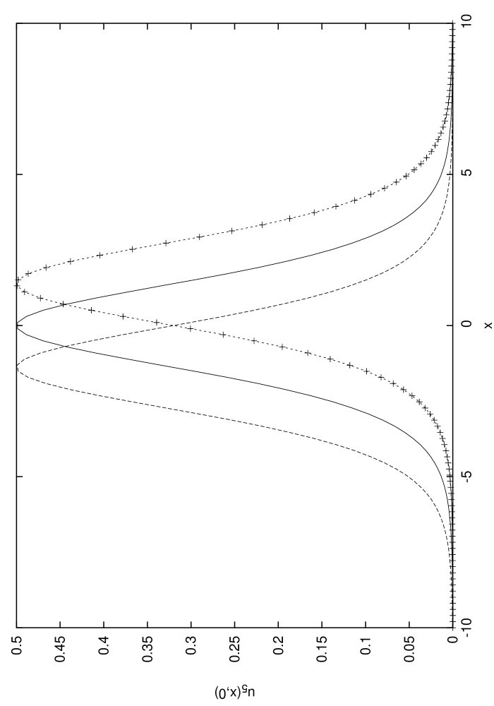
Figure 1: Variation of $u_{5}(x,0)$ with $x$

All the curves in the figure are of $sech^{2}$ shape indicating that solution obtained from $(63)$ have indeed solitary wave properties. The solid curve for $c_{0}=1$ and $c_{1}=1$ is centred at the point $x=0$. If $c_{0}$ and $c_{1}$ are made unequal, the centre of the soliton moves either to the left or to the right. In particular, for $c_{0}>c_{1}$, the shift of the centre is towards the right and we have a reverse situation for $c_{0}<c_{1}$. We have displayed this property by using a dashed curve with cross $(c_{0}=4$ and $c_{1}=1)$ and a simple dashed curve $(c_{0}=1$ and $c_{1}=4)$. V. Conclusion

Fifth-order nonlinear evolution equations, on the one hand, have a host of connections with other important integrable equations and, on the other hand, can not be solved by simple analytical methods. These two points inspired us to construct a general fifth-order equation which follow from a Lagrangian. It is often desirable that equations of mathematical physics should be derivable from an action principle because a non-Lagrangian system does not allow one to carry out a linear stability check [24] as well as to derive a field theory [25] for particles described by its solutions. The Lagrangian approach to nonlinear evolution equations is quite interesting because here one can derive all physico-mathematical results from first principles [8]. Based on the fifth-order Lagrangian equation we derived an integrable hierarchy. As a test of integrability we provided a Lax representation and constructed two compatible Hamiltoinan structures.

We treated the third- and fifth-order equations in the hierarchy by the homogeneous balance method [15] to obtain analytical results for soliton solutions. Ideally, we could have tried the bi-linear method of Hirota [26] to deal with the problem because this method is very convenient for finding single- and multi-soliton solutions of nonlinear evolution equations. For higher-order equations, Hirota transformation often leads to multilinear representation [27]. This tends to pose problems in solving the equations. The homogeneous balance method, on the other hand, does not involve any new mathematical complication as one moves from lower- to higher-order equations. Admittedly, the algebra become more and more involved as we go up the ladder inside the hierarchy. The symbolic computations facilities like the Mapple and Mathematica can be used to circumvent algebraic complications.

Acknowledgement. This work is supported by the University Grants Commission, Government of India, through grant No. F.10-10/2003(SR).

[1] K. Nakkeeran, K. Porsezian, P. Shanmugha Sundaram and A. Mahalingam, Phys. Rev. Lett. 80, 1425 (1998).

[2] U. Al Khawaja, H. T. C. Stoof, R. G. Hulet, K. E. Strecker, and G. B. Patridge, Phys. Rev. Lett. 89, 200404 (2002).

[3] M. N. Özer and F. T. Döken, J. Phys. A.: Math. Gen. 36, 2319 (2003).

[4] M. N. Özer and I. Dağ, Hadronic. J. 24, 195 (2001).

[5] P. D. Lax, Comm. Pure Appl. Math. 21, 467 (1986).

[6] K. Sawada and T. Kotera, Prog. Theo. Phys. 51, 1355 (1974).

[7] D. J. Kaup, Stud.Appl.Math. 62, 189 (1980); B. Kupersmidt, Commun. Math. Phys. 99, 51 (1988).

[8] P. Rosenau and J. M. Hymann, Phys. Rev. Lett. 70, 564 (1993); B. Talukdar, J. Shamanna and S. Ghosh, Pramana. J. Phys. 61, 99 (2003); S. Ghosh, U. Das and B. Talukdar, Int. J. Theor. Phys. 44, 363 (2005)

[9] W. Hong and Y. Jang, Z. Naturforsch. 54a, 549 (1999).

[10] R. M. Santili, Foundations of Theoretical Mechanics I (Springer-Verlag, New York, 1984).

[11] F. Magri, J. Math. Phys. 19, 1548 (1971).

[12] B. Talukdar, S. Ghosh, J. Shamanna and P. Sarkar, Eur. Phys. J. D21, 105 (2002); B. Talukdar. S. Ghosh and U. Das, J. Math. Phys. 46, 043506 (2005).

[13] D. Anderson, Phys. Rev. A. 27, 3135 (1983).

[14] F. Cooper, C. Lucheroni, H. Shepard and P. Sodano, arxiv:hep-ph/9210226 v1, 9 Oct 92.

[15] M. Wang, Phys. Lett. A. 199, 169 (1995); ibid 213, 279 (1996); 216, 67 (1996).

[16] P. J. Olver, Application of Lie Groups to Differential Equation, (Springer-Verlag, NY, 1993).

[17] M. Ito, J. Phys. Soc. Japan 49, 771 (1980).

[18] F. Calogero and A. Degasperis, Spectral Transform and Soliton (North-Holland Publising Company, New York, 1982).

[19] K. Chadan and P. C. Sabatier, Inverse problems in Quantum Scattering Theory (2nd ed, Springer, New York, 1989).

[20] V. E. Zakharov and L. D. Faddeev, Funct. Anal. Phys. 5, 18 (1971).

[21] C. S. Gardner, J. Math. Phys. 12, 1548 (1971).

[22] S. Ghosh, B. Talukdar and J. Shamanna, Czech. J. Phys. 53, 425 (2003).

[23] C. S. Gardner, J. M. Greene, M. D. Kruskal and R. M. Miura, Phys. Rev. Lett. 19, 1095 (1967).

[24] B. Dey and A. Khare, J. Phys. 33, 5335 (2000).

[25] S. A. Hojman and L. C. Shepley, J. Math. Phys. 32, 142 (1990).

[26] R. Hirota, Phys. Rev. Lett. 27, 1192 (1971).

[27] J. Hietarinta in Nonlinear Dynamics: Integrability and Chaos ed. M. Daniel, K. M. Tamizhmani and R. Sahadevan (Narosa Publising House, New Delhi (2000)).