Surrogate data method applied to nonlinear time series

Abstract

The surrogate data method is widely applied as a data dependent technique to test observed time series against a barrage of hypotheses. However, often the hypotheses one is able to address are not those of greatest interest, particularly for system known to be nonlinear. In the review we focus on techniques which overcome this shortcoming. We summarize a number of recently developed surrogate data methods. While our review of surrogate methods is not exhaustive, we do focus on methods which may be applied to experimental, and potentially nonlinear, data. In each case, the hypothesis being tested is one of the interests to the experimental scientist.

and

1 Introduction

1.1 Overview

The physical phenomena in the real world are usually attributed to certain causalities [11]. With different causalities, the corresponding phenomena, often captured in the time series of measurement, might diverge significantly as illustrated in Fig. 1: They could be irregular fluctuations as shown in panel (a), or pseudo-periodic data in panel (b), or the mixture, i.e., irregular fluctuations with periodic trends as indicated in panel (c).

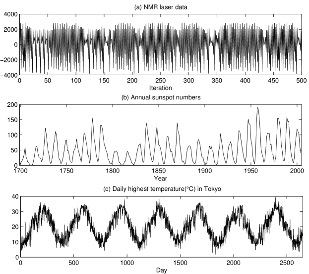
Figure 1: (a) Nuclear magnetic resonance (NMR) laser data, (b) Annual sunspot numbers from the year 1700 to 2004, and (c) Daily highest temperature in Tokyo from 1 January 1998 to 31 March 2005.

To understand the underlying mechanisms responsible for generating those different time series in Fig. 1, one needs to reply some elementary questions first: are the data linear or nonlinear, stochastic or deterministic, pseudo-periodic or chaotic? To explore the possible answers, the method of Monte Carlo hypothesis test [2, 10], or surrogate data test equivalently [6, 30, 33, 36, 38], is often applied. This method has become a useful tool to validate the results of dynamical analysis, and thus help understand the causal processes underlying the experimental data. For example, if through the method one finds that irregular fluctuations are not random variables, then it immediately implies that there exists some kind of dynamical (deterministic) structure. Therefore a consequential conclusion is that, it is possible to build deterministic models (or model systems) from the time series.

The focus of this section is to introduce the framework of Monte Carlo hypothesis test. Moreover, we will discuss some important concepts associated with the components that form the framework, which will be frequently applied in our later analysis.

1.2 Monte Carlo hypothesis test

Null hypothesis tests use statistical measures of the underlying system to determine the probability that a proposed hypothesis is true (or false) [44]. The common procedures include [7]:

1. Formulate the null hypothesis of interest, the alternative hypothesis and the potential risks associated with a decision.

2. Choose a test statistic.

3. Compute the frequency distribution of the test statistic under the null.

4. With the guide of the frequency distribution, choose certain criterion to determine whether to reject the hypothesis or not.

It is easy to see that the framework of hypothesis testing consists of the null hypothesis, the test statistic, the frequency distribution of the test statistic, and the discriminating criterion that determines whether to reject the null hypothesis or not. In order to obtain the frequency distribution of the test statistic, traditionally one would need to carefully choose the test statistic such that it follows a well known distribution. But in practice, on one side it might be difficult to find the refined statistics for tests in many situations; on the other, with modern computers the computer-intensive methods become feasible and popular [23]. Hence, the concept of Monte Carlo hypothesis test naturally appeared [2, 10]. The basic idea is to produce a number of different realizations under the null through Monte Carlo simulation. In practice these realizations are usually generated from the original experimental data, but not really ever observed, therefore they will also be called the surrogate data in the later. From the ensemble of the surrogates, one could calculate the empirical distribution and the confidence interval of the test statistic. In this sense, the frequency distribution will essentially depend on the surrogate generation algorithm (and the chosen statistic of course). Therefore one could also say that the surrogate algorithm is one of the elements that form a null hypothesis test, as we do in the later.

1.3 Pivotality and constrained-realization surrogates

For the convenience of our later discussion, we need to introduce some terminologies. Following the notation in [33, 38], let $\mathcal{F}$ be the set of all the possible processes for the problem under consideration. Also let $\phi$ be the formulated null hypothesis and $\mathcal{F}_{\phi}$ the set of processes that are consistent with the null $\phi$. If $\mathcal{F}_{\phi}$ consists of only one element, then the null hypothesis $\phi$ is called simple, otherwise it is called composite.

Given a composite null hypothesis $\phi$ and a process $F$ consistent with $\phi$, let us denote the chosen test statistic by $T$, and the corresponding probability distribution function (PDF) under the null hypothesis by $P_{T,F}(t)\equiv Prob(T<t|F\in\mathcal{F}_{\phi})$. If for any two processes $F_{i}$ and $F_{j}$ ($i\neq j$) in the set $\mathcal{F}_{\phi}$, one has that $P_{T,F_{i}}(t)=P_{T,F_{j}}(t)$, then the statistic $T$ is said pivotal; otherwise it is non-pivotal.

A remarkable advantage of test statistics which are pivotal, as can be seen from the definition, is that one will always obtain the same statistic distribution $P_{T}(t)$, which is independent of the process $F$ chosen from the set $\mathcal{F}_{\phi}$. Therefore adopting a pivotal test statistic might significantly reduce the difficulty in devising the algorithm to produce surrogates of the null [31]. However, if the test statistic is non-pivotal, then there is no guarantee that $P_{T,F_{i}}(t)=P_{T,F_{j}}$ holds for arbitrary processes $F_{i}$ and $F_{j}$ in $\mathcal{F}_{\phi}$. Suppose that the time series $\mathbf{d}=\{d_{i}\}_{i=1}^{n}$ under test is generated from a process $F_{d}\in\mathcal{F}_{\phi}$, then in order to avoid possible false rejection of the null hypothesis , it is usually required, as the sufficient condition, that the process $F_{s}$ producing the surrogate data satisfies $F_{s}=F_{d}$ . Surrogates generated from such processes are called constrained realizations; otherwise it is said non-constrained. Obviously, given a set of constrained-realization surrogates $\{\mathbf{s_{1},s_{2},...}\}$, any adopted test statistic $T$ will appear as if it were pivotal for the processes $\{F_{d},F_{s_{1}},F_{s_{2}},...\}$.

In the following sections, we will introduce various applications of the Monte Carlo hypothesis test method. One of the popular applications is to detect nonlinearity in a time series, as described in [20, 35, 36, 38]. Other applications include the detection of aperiodicity [12, 32, 37] and the correlation between irregular fluctuations with long term trends [21]. As an important, and possibly the most attractive component, the well-tailored surrogate generation algorithm associated with the hypothesis deserves to receive great attention. In fact, because of its importance, the Monte Carlo hypothesis test method is often called surrogate data test, or surrogate data method [6, 30, 33] in the literature. In this review we use these two terms interchangeably.

There are already some excellent introductory works covering the topic of the surrogate data method (for example [6, 30, 33]), therefore we will not provide excessive detail in this paper. Instead, we will dedicate our effort to introducing some of more recent progress. The readers are referred to the broad literature, much of which is cited here, for further detail. The three reviews [6, 30, 33] are particularly recommended.

2 Surrogate test for detection of nonlinearity

A rational step before the application of nonlinear time series methods is to identify the presence of nonlinearity. For this purpose, one could employ the direct detection strategy, that is, in order to detect nonlinearity, one adopts some characteristic nonlinear statistics, such as the correlation dimension, the Lyapunov exponent, the continuity, and so on [14, 15, 43], as the discriminating measures in the belief that these statistics reveal the essential behaviors of nonlinear systems. This strategy, however, may encounter a few disadvantages in practice. On one hand, in certain situations the characteristic nonlinear statistics do not play the role well as the unequivocal identifiers of the underlying systems [33]. Take the correlation dimension [8, 9] as an example, it was shown that some linear stochastic processes with simple power law spectra would also have finite non-integer values as many nonlinear systems do [24], thus one would fail to distinguish between linearity and nonlinearity by simply examining the values of the correlation dimension. On the other hand, given only a limited amount of the realizations of the underlying systems, it is often difficult to evaluate the reliability of the test results based on the direct detection strategy. The situation becomes even worsen with the presence of noise, which, often is the case, will reduce the discriminating power of the characteristic statistics. Thus one is forced back to the aforementioned scenario, i.e., the adopted characteristic statistic fails to unequivocally identify the underlying system. As an example, let us consider the (largest) Lyapunov exponent. Theoretically its value shall be zero for a periodic orbit. However, if the periodic orbit is perturbed by noise components, the value of the Lyapunov exponent might slightly increase and become positive, which is often deemed as the sign of chaos and therefore possibly engenders misleading conclusion.

An alternative strategy for nonlinearity detection is the surrogate data methods, as an application of the Monte Carlo hypothesis test. The test procedures go as follows, one first proposes a null hypothesis which usually assumes that the time series is initially generated by a linear stochastic process. With the null hypothesis, one produces an ensemble of surrogate data based on the original time series. Then one chooses a proper test statistic in the sense that, if the original data is consistent with the null hypothesis, the statistic of the original data shall follow the same distribution as those of the surrogates, otherwise it shall appear atypical to the distribution. After calculating the test statistic, one inspects whether the statistic value of the original data appears typical to the distribution of the surrogates according to certain discriminating criterion. If the answer is no, one rejects the null with certain confidence level (depending on the chosen discriminating criterion, as will be discussed in the later), which implies that the data in test is very likely to be nonlinear.

In this section, we will first review the the hierarchical surrogate data tests for nonlinearity detection proposed by Theiler et al. [36, 38]. We will also introduce other surrogate data methods [20, 28, 29], which essentially follow the same hierarchical framework but differentiate in the way of surrogate generation, as will be explained in the following.

2.1 The hierarchical surrogate data tests

Here we confine our discussion to stationary irregular time series. With the data, as the first step of analysis we want to detect the potential nonlinearity in it. Of course it is also possible that the irregular data is produced from a linear stochastic system, or a linear deterministic system contaminated by noise. Since the stationary data generated by a linear deterministic system appear either periodic or constant, even with noise components it is trivial to distinguish between linear stochastic and deterministic cases if the noise level is not extremely high . Therefore in the later we will only consider the scenario that the stationary irregular time series is generated from either a linear stochastic process or a nonlinear stochastic or deterministic process. Following the aforementioned procedures, we will introduce one by one the basic elements that form the framework of null hypothesis tests.

2.1.1 Null hypotheses

The basic assumption is that the time series under test is from a linear stochastic noise process, either i.i.d. (independent and identically distributed) or correlated (in the general form of an auto-regressive moving average $ARMA$ process). But note that, it is possible to introduce nonlinearity into the original linear data during the measurement step by letting the original data pass through a nonlinear filter [30]. With this consideration, one could formulate the following hierarchical composite hypotheses (or those equivalently stated in [6, 33, 36, 38]), as shown in Fig. 2:

Figure 2: Schematic representation of the hierarchical hypotheses and their alternatives.

• Null Hypothesis 0 (NH0): The data in test are i.i.d. noise with unknown mean and variance.

• Null Hypothesis 1 (NH1): The data in test are produced from a linear stochastic process in the form of an $ARMA$ model with unknown parameters, which is essentially a linear filter of the i.i.d noise.

• Null Hypothesis 2 (NH2): The data in test are obtained by applying a static and monotonic nonlinear filter to the time series originally generated by an $ARMA$ process.

2.1.2 Test statistic

In principle one shall choose the statistics in a way that measures of the original data and the surrogates shall appear consistent if the null hypothesis is true; otherwise they will reveal the discrepancy. For this purpose, one of the popular choices in the literature is the correlation dimension, since it was shown that the correlation dimension is a pivotal statistic for the hierarchical null hypothesis tests for nonlinearity detection [31, 33]. Of course, there are also many other proper candidates. And in general, the discriminating powers of the test statistics may vary from case to case [27].

2.1.3 Surrogate generation algorithms

Broadly speaking, there are two strategies to generate surrogate data. One is to first build a parametric model based on the null hypothesis (rather than the original data), and then use the model to produce the surrogates. The other one is to seek a nonparametric model to produce surrogates consistent with the null hypothesis, which is especially useful for the test of a composite null hypothesis and will thus be the focus in our later discussions. Of course, parametric algorithms can also be constructed for composite hypotheses as long as one could find suitable pivotal test statistics. In such situations, the hypothesis which one can test is that, the data are consistent with a particular parametric model (possibly fitted to the data), or any other model with the same frequency distribution of the test statistic. This parametric approach can be particularly useful if one is interested in providing a behavior (or dynamics) based test of the suitability of a particular model. However, such parametric algorithms are often non-constrained and we will not consider them in this review. The interested readers are referred to [6, 31, 35, 31].

Now let us begin introducing the nonparametric (and constrained) surrogate generation algorithms that correspond to the above hierarchical null hypotheses:

• Algorithm 0: To produce i.i.d. surrogates, one only needs to randomly shuffle the original data.

• Algorithm 1: To produce linear stochastic surrogates, one first applies the Fourier transform to the original data to obtain the corresponding moduli and phases. Then one keeps the moduli but replace the phases by random numbers uniformly drawn from the interval $(-\pi,\pi]$. Finally one applies the inverse Fourier transform to the coefficients with preserved moduli but randomized phases. Thus obtained data are the desired surrogates.

• Algorithm 2: To produce surrogates consistent with NH2, one first needs to invert the static and monotonic nonlinear filter to obtain the original linear stochastic data, then applies Algorithm 1 to generate interim surrogate data of the linear data, and finally introduce the nonlinear filter back into the interim surrogates to obtain the final surrogates.

The surrogates produced from the above algorithms will preserve the amplitude distribution of the original data as we expect. However there also exist a few defects in practice. One problem is that, for surrogates generated by Algorithm 1, their power spectra will often deviate from that of the original data. As a remedy, Schreiber and Schmitz [28] suggested to repeat the surrogate generation procedures until the difference between the power spectra reaches certain stopping criterion. Another problem is that, to apply the discrete Fourier transform, the data has to be assumed periodic. Therefore the wraparound artifact [6, 39] will be introduced. A possible remedy, as suggested in [6, pp. 238-240], is to conduct limited phase randomization. Another remedy is to avoid adopting the Fourier transform, as will be discussed later.

2.1.4 Discriminating criterion

Since the exact knowledge of the statistic distribution is often not available, one will resort to certain discriminating criterion to help make the decision and determine the corresponding confidence level (if to reject). The popular discriminating criteria in the literature include two classes: parametric and nonparametric. The parametric criterion assumes that the statistic follows a Gaussian distribution, and the distribution parameters, i.e. the mean and the variance, would be estimated from the finite samples. One can determine whether to reject the null by examining whether the statistic of the original time series follows the statistic distribution of the surrogates, while the corresponding confidence level of inference can be calculated from the estimated statistic distribution; The nonparametric criterion [40] examines the ranks of the statistic values of the original time series and its surrogates. Supposes that the statistic of the original time series is $T_{0}$ and the surrogate values are $\{T_{i}\}_{i=1}^{N}$ given $N$ surrogate realizations. Then if the statistic of both the original time series and the surrogates follows the same distribution, the probability is $1/(N+1)$ for $T_{0}$ to be the smallest or largest among all of the values $\{T_{0},T_{1},...,T_{N}\}$. Thus if $N$ is large, when one finds that $T_{0}$ is smaller or larger than all of the values in $\{T_{i}\}_{i=1}^{N}$, it is quite possible that $T_{0}$ instead follows a different distribution from that of $\{T_{i}\}_{i=1}^{N}$. Hence the criterion rejects the null hypothesis whenever the original statistic $T_{0}$ is the smallest or largest among $\{T_{0},T_{1},...,T_{N}\}$, the false rejection rate is considered as $1/(N+1)$ for one-sided tests and $2/(N+1)$ for two-sided ones.

2.2 Other methods to generate surrogates

2.2.1 The temporal shift algorithm

The basic idea of the temporal shift algorithm [12, 20] goes as follows: For two independent time series ${\bf x}=\{x_{i}\}_{i=1}^{N}$ and ${\bf y}=\{y_{i}\}_{i=1}^{n}$, if they are produced from a same linear stochastic process, then the additions ${\bf z}=\{z_{i}:z_{i}=\alpha x_{i}+\beta y_{i}\}_{i=1}^{N}$ for arbitrary real scalar coefficients $\alpha$ and $\beta$ will also follow the same linear process, although possibly with different initial conditions. However, if ${\bf x}$ and ${\bf y}$ are from a nonlinear (stochastic or deterministic) process, in general adding them together will increase the complexity. Thus their additions ${\bf z}$ may behave different from ${\bf x}$ and ${\bf y}$. And by adopting a proper test statistic, one may detect this difference.

In practice, if only given a single time series ${\bf d}=\{d_{i}\}_{i=1}^{N}$, then in order to produce surrogates, one could extract two subsets from the original data, for example, ${\bf d_{1}}=\{d_{i}\}_{i=1}^{N-\tau}$ and ${\bf d_{2}}=\{d_{i}\}_{i=1+\tau}^{N}$, where parameter $\tau$ is the temporal shift-or more precisely, index shift-between ${\bf d_{1}}$ and ${\bf d_{2}}$, and is often required to decorrelate ${\bf d_{1}}$ and ${\bf d_{2}}$. The surrogates ${\bf s}$ are produced according to the formula $s_{i}=\alpha d_{i}+\beta d_{i+\tau}(i=1,2,...,N-\tau)$, by either varying the temporal shift $\tau$, or randomizing the coefficients $\alpha$ and $\beta$, or the combinations. In principle, there is no requirement for the coefficients $\alpha$ and $\beta$. But note that, if the ratio $\alpha/\beta\rightarrow 0$ or $\infty$, then roughly the surrogates ${\bf s}=\alpha{\bf d_{1}}+\beta{\bf d_{2}}\propto{\bf d_{2}}$ or ${\bf d_{1}}$. Therefore whether the original data is consistent the null hypothesis or not, the produced surrogates will look very close to it. Consequently, even if the null hypothesis does not actually hold, the test statistic may fail to detect the tiny difference between the surrogates and the original data. Thus spurious results will appear in these situations. To avoid this problem, we suggest that the ratio $\alpha/\beta$ takes moderate values. For detail, see [12].

From the above discussions, it is easy to find that the temporal shift algorithm actually utilizes the fact that the superposition principle is applicable to linear processes rather than nonlinear ones. And with this fact, one could avoid applying the Fourier transform to the original data and thus circumvent the consequential wraparound artifact. One may also note that, in contrast to the standard algorithms (i.e., Algorithm 0-2 and the iterative version of Algorithm 2) , the surrogates produced by the temporal shift algorithm do not exactly preserve the amplitude distribution of the original data. However, since the algorithm ensures that the surrogates are generated from the same process under the null hypothesis, it is still a constrained-realization surrogate generation algorithm. In our viewpoint, the elimination of the restriction to preserving the amplitude distribution is actually an advantage of the new algorithm, which makes the algorithm more flexible and efficient to produce surrogates.

2.2.2 The simulated annealing method

Simulated annealing [16] is a stochastic approach that mimics the physical process to solve the combinatorial optimization problems. Physically, the annealing process starts from a high temperature that melts the solids, then one gradually decreases the temperature. If the variation amplitude of the temperature is small enough, after a sufficiently long time all of the particles will reach the ground state so that the system energy is minimal. The simulated annealing bears an analogy to the physical process. As the initial condition, the control parameter (analogy to the temperature) adopts a proper value. Then one needs to carefully tune the parameter according to certain cooling schedule. At each parameter value, by devising an appropriate neighborhood generation (or state updating) mechanism and acceptance criterion, the transitions between the accepted states prove to form a homogeneous Markov chain. And the global optimal state(s), which minimize(s) or maximize(s) the cost function (analog to the system energy), will be achieved as the control parameter tends to zero. For detail, see, for example, [1, 42].

As we have mentioned previously, surrogates produce by Algorithm 2 preserve the amplitude distribution of the original data but differentiate in the power spectra. One remedy for this problem is to iterate the surrogate generation procedures for a number of times until certain criterion is satisfied. However, usually there is no guarantee that the chosen criterion is the best, therefore it is possible that the iterative algorithm only engenders sub-optimal solutions (i.e., local minima) or even worse. For this reason, applying the simulated annealing method for surrogate generation, in contrast, will often achieve better performance, as pointed out by Schreiber [29]. However, in some situations, this approach can be time consuming and provide limited benefit [33].

Because the linear autocorrelations are directly related to the power spectrum [3], in configuration of the simulated annealing it is natural to choose, as the cost function, the norm of the difference between the linear autocorrelations of the original and the simulated data (see Eq.(2) of [29]). The (accepted) simulated data is updated by exchanging the pairs of the former one, while the expected surrogate is the final simulated data when the stopping criterion is reached . Hence it is easy to arrive the conclusion that thus generated surrogates are also constrained realizations in the sense that they preserve the amplitude distribution of the original data.

In practice, one inherent advantage to apply the simulated annealing method is that, after adequate cooling for the control parameter, the obtained solution could reach a local minimum sufficiently close to the global one. Another advantage is that it does not need to invert the nonlinear filter for the test of NH2. Of course, there is also one obvious disadvantage, that is, depending on the size of the problem and the configuration of the algorithm, the computational time might substantially increase as often the case.

3 Surrogate test for detection of aperiodicity

In the previous section we have described the tests that can be applied to arbitrary time series data. We now confine our discussion to pseudo-periodic data. By pseudo-periodic data we mean those time series that exhibit strong periodic trends manifesting as clear spikes in the frequency domain [33] (see Figure 1(a) and (c) ). The underlying systems of pseudo-periodic data can be periodic orbits contaminated with observational or dynamical data, or oscillatory chaotic systems (for example the Rössler system). In this sense, one could also apply the surrogate data method to detect chaos in a pseudo-periodic time series, which will be the focus of this section.

3.1 The cycle shuffled algorithm

Here let us first specify the null hypothesis, which assumes that there are no temporal correlations at all between the spike-and-wave patterns (i.e., the individual cycle patterns) of the pseudo-periodic time series [37]. Obviously, any purely periodic time series is consistent with the hypothesis. However, if there exists perturbations to the periodic orbits, then it requires that those inter-cycle perturbations are also uncorrelated at all (for example, the i.i.d noise), which is a stronger constraint than that of the null hypothesis to be introduced in the next subsection.

Since there are no temporal correlations between individual cycle patterns, similar to the idea of block bootstrap [18] to decompose and shuffle individual blocks, the natural way to produce pseudo-periodic surrogates is to first extract the individual cycles from the pseudo-periodic time series and then randomly shuffle these cycles. For this reason, this method is often called cycle shuffled algorithm. Note that, although not explicitly specified in the null hypothesis, in order to let the algorithm produce constrained realizations, it requires that intra-cycle dynamics of the individual cycles distributes periodically.

Theoretically the cycle shuffled algorithm is very simple, but there is a practical problem in implementation, which essentially lies in the difficulty in extracting the individual cycles from the test data. Given a pseudo-periodic time series, shuffling the split cycles will often lead to the spurious discontinuity. To eliminate this phenomenon, one could vertically shift the individual cycles, but it often turns out to make the data become non-stationary and thus generate artificial long term correlation (see, for example, the illustrations in [33]). In the following we will introduce another algorithm that produces surrogates from a different viewpoint and avoids the above problems. Moreover, if one is interested primarily in the variation between cycles, it may be better to study that directly [46].

3.2 The temporal shift algorithm

Here the null hypothesis under test is that the pseudo-periodic time series is produced from a periodic orbit perturbed by noise components that are identically distributed and uncorrelated for large enough temporal shifts [12]. This null hypothesis is slightly more general than that in the previous subsection in the sense that, it does not require that there are no temporal correlations between the individual cycles .

Note that, adding together two subsets of the same periodic time series will lead to a new periodic data, while for chaotic time series applying the same transformation will usually increase the complexity. With this property, one could adopt the temporal shift algorithm as well to produce the surrogates under the hypothesis, i.e., given a $N$-point pseudo-periodic time series ${\bf d}=\{d_{i}\}_{i=1}^{N}$, one could generate the surrogates ${\bf s}$ according to the formula $s_{i}=\alpha d_{i}+\beta d_{i+\tau}(i=1,2,...,N-\tau)$ with proper coefficient ratios $\alpha/\beta$. However, there is still an important difference, that is, for pseudo-periodic time series usually the temporal shift algorithm is not constrained. This is because in this situation the surrogates only preserve the periodicity but not necessarily the cycle pattern (see Fig. 3 for an illustration). Therefore the surrogates, although also periodic, may not come from the same underlying system as that of the original data. With this consideration, one shall choose a pivotal test statistic with robust performance against noise in calculation. An example of such choices is the correlation dimension evaluated by the Gaussian kernel algorithm (GKA), as described in [4, 45].

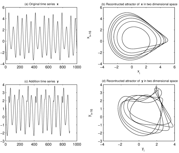
Figure 3: An illustration of that the addition of two subsets of a periodic time series does not preserve the original cycle pattern. Panel (a) Original period 6 time series ${\bf x}=\{x_{i}\}_{i=1}^{1000}$ from the Rössler system; (b) The reconstructed attractor in two dimensional embedding space $x_{i+16}$ vs. $x_{i}$; (c) Addition time series ${\bf y}=\{y_{i}:y_{i}=x_{i}+x_{i+100}\}_{i=1}^{900}$; (d) The reconstructed attractor in two dimensional embedding space $y_{i+16}$ vs. $y_{i}$. From the reconstructed attractor [19, 26, 34] in panel (d), one can find that the addition time series is also period 6, however its cycle pattern differs from that of the original time series.

3.3 The attractor trajectory surrogate algorithm

The attractor trajectory surrogate (ATS) algorithm produces surrogates by inferring the underlying systems from a local model, and contaminating a trajectory on the attractor with dynamical noise [33]. In this way, the surrogates preserve the gross scale dynamics of the original data but destroy the fine scale one.

Examples of the ATS algorithm can be found in [5, 32, 41]. Here we only introduce the pseudo-periodic surrogate (PPS) algorithm [32] which is designed for detection of the null hypothesis that assumes the time series from a periodic orbit with uncorrelated dynamical noise.

Given a scalar time series ${\bf z}=\{z_{i}\}_{i=1}^{N}$, the procures for surrogate generation go as follows [32, 33]:

1. Choose proper embedding dimension $d_{e}$ and time delay $\tau$ for time delay embedding reconstruction [19, 26, 34]. By reconstruction based on the original data ${\bf z}$, one obtains a set of delay vectors ${\bf V}=\{{\bf v}_{i}\}_{i=1}^{d_{w}}$ with delay vector ${\bf v}_{i}=[z_{i},z_{i+1},...,z_{i+(d_{e}-1)\tau}]^{T}$ and the embedding window $d_{w}=N-(d_{e}-1)\tau$.

2. Randomly choose a delay vector ${\bf\chi}_{0}\in{\bf V}$ for initialization.

3. Let index $k$ start from $k=1$.

4. Let ${\bf\chi}_{k}$ be the current delay vector in operation. Search in ${\bf V}$ the neighbors of ${\bf\chi}_{k}$ and randomly pick out one as the successor of ${\bf\chi}_{k}$, which is denoted by ${\bf\chi}_{k+1}$.

5. Take ${\bf\chi}_{k+1}$ as the current operation vector. Repeat the procedure in step 4 until index $k$ reaches the specified length, say, $M$.

6. The surrogate data ${\bf s}=\{s_{i}:s_{i}=(\chi_{i})_{1}\}_{i=0}^{M}$, where $(\chi_{i})_{1}$ denotes the first element in vector $\chi_{i}$.

It was shown [33, p.160] that the surrogates ${\bf s}$ produced through the above procedures share the same vector field as the original data ${\bf z}$ but are contaminated with dynamical noise. However, the produced surrogates may not strictly preserve the gross scale dynamics of the original data as we observed in practice. In this sense, the surrogates are not constrained realizations, therefore in tests one needs to choose a pivotal statistic (e.g., the correlation dimension as aforementioned).

4 Surrogate test for detection of correlations between irregular fluctuations

A new application of the surrogate data method is to detect correlations between irregular fluctuations possibly with a long term trend [21]. The corresponding null hypothesis is that irregular fluctuations are independently distributed, which differentiates NH0 of Section 2 in that it does not require the identical distribution of the fluctuations.

Similar to the idea of the attractor trajectory surrogate (ATS) algorithm, the surrogate generation algorithm devised in [21] also aims to preserve the global behavior (e.g., the trend) but destroy the local one. In the following let us explain in more detail.

Given a scalar data ${\bf d}=\{d_{i}\}_{i=1}^{N}$, let the index set be ${\bf h}=\{h_{i}:h_{i}=i\}_{i=1}^{N}$ such that $d_{i}=d_{h_{i}}$, then the concrete steps for implementation of the idea include:

1. Perturb the original index set ${\bf h}$ with Gaussian random numbers $\{\xi_{i}\}_{i=1}^{N}$ so as to obtain a real number set ${\bf r}=\{r_{i}:r_{i}=h_{i}+A\xi_{i}\}_{i=1}^{N}$.

2. Sort ${\bf r}$ in the ascendant order to produce a new data set ${\bf t}$. Re-ordering the index set ${\bf h}$ will lead to the disturbed index set ${\bf k}=\{k_{i}\}_{i=1}^{N}$, which satisfies $t_{i}=r_{k_{i}}$.

3. The surrogate data ${\bf s}=\{s_{i}\}_{i=1}^{N}$ is obtained by letting $s_{i}=d_{k_{i}}$.

By choosing a proper amplitude $A$, typically the irregular fluctuations will only slightly move from the positions in the original data, therefore the generation mechanism is called small-shuffle surrogate (SSS) algorithm. But note that, although the surrogates ${\bf s}$ preserve the amplitude distribution of the original data ${\bf d}$, usually the surrogates are not constrained realizations. This is because the irregular perturbations are possibly not identically distributed, and locally shuffling the irregular perturbations may not exactly preserve the global dynamics. Thus, one needs to carefully choose the test statistics, which may be the linear autocorrelation function or the average mutual information as suggested in [21].

5 Summary

In the above sections we have reviewed the concept of surrogate data tests, the primary components that form the framework of this method, and some important properties of these components. We have also reviewed the applications of the surrogate data method, with the emphasis on some recently developed surrogate generation algorithms.

In all of the applications, since the specified null hypotheses are composite, it is required that the surrogate generation algorithms are nonparametric and work for any process consistent with the hypothesis. Consequently, the broader range of the underlying processes a composite null hypothesis may cover, the more difficult it is to design the corresponding nonparametric surrogate algorithm. This fact limits the applications of the surrogate data method to detect many other interesting properties.

Another challenge is the design of a proper test statistic. The problem comes not only from the requirement of pivotal-ness when the surrogates are not constrained realizations, but also from the expectation that one obtains the exact confidence level to reject a null hypothesis. Although simple in handle, the two discriminating criteria described in Section 2 actually cannot lead to inferences with exact confidence levels (see the discussion in [13]). The solution to this problem requires that one seeks the full knowledge of the distribution of the test statistic, which is often infeasible, even only at the asymptotic level, for many nonlinear statistics.

6 Acknowledgements*

This research was supported by Hong Kong University Grants Council Competitive Earmarked Research Grant (CERG) No. PolyU 5235/03E.

References

- [1] E. Aarts and J. Korst, Simulated Annealing and Boltzmann Machines : A Stochastic Approach to Combinatorial Optimization and Neural Computing (Wiley, 1989).
- [2] G.A. Barnard, J. Roy. Statis Soc. B 25, 294 (1963).
- [3] G.E.P. Box, G.M. Jenkins and G.C. Reinsel, Time Series Analysis: Forecasting and Control 3rd Ed. (Prentice-Hall, 1994).
- [4] C. Diks, Phys. Rev. E 53, 4263 (1996).
- [5] K. Dolan, A. Witt, M.L. Spano, A. Neiman and F. Moss, Phys. Rev. E 59, 5235 (1999).
- [6] A. Galka, Topics in Nonlinear Time Series Analysis with Implications for EEG Analysis (World Scientific, 2000).
- [7] P. Good, Permutation, Parametric, and Bootstrap Tests of Hypotheses 3rd Ed. (Springer, 2005).
- [8] P. Grassberger and I. Procaccia, Phys. Rev. Lett. 50, 346 (1983).
- [9] P. Grassberger and I. Procaccia, Physica D 9, 189 (1983).
- [10] A.C.A. Hope, J. Roy. Statis Soc. B 30, 582 (1968).
- [11] K. Judd, Building optimal models of time series, in Chaos and its Reconstruction (ed. G. Gousebet, S. Meunier-Guttin-Cluzel and O. Menard) (Nova Science Pub Inc, 2003).
- [12] X. Luo, T. Nakamura and M. Small, Phys. Rev. E 71: 026230 (2005).
- [13] X. Luo, J. Zhang and M. Small, submitted.
- [14] D.T. Kaplan and L. Glass, Phys. Rev. Lett. 68, 427 (1992);
- [15] D.T. Kaplan, Physica D 73, 38 (1994).
- [16] S. Kirkpatrick, C.D. Gelatt and M.P. Vecchi, Science 220, 671 (1983).
- [17] D. Kugiumtzis, Phys. Rev. E 62, 25 (2000).
- [18] H.R. Künsch, Annals of Statistics 17, 1271 (1989).
- [19] R. Man̂é, On the dimension of the compact invariant sets of certain non-linear maps, in Lecture Notes in Math. Vol. 898 (Springer, New York, 1981).
- [20] T. Nakamura, X. Luo and M. Small, Phys. Rev. E 72: 055201 (2005).
- [21] T. Nakamura and M. Small, Phys. Rev. E 72: 056216 (2005).
- [22] A.I. Mees, Nonlinear Dynamics and Statistics (Birkhäuser, 2000).
- [23] E.W. Noreen, Computer-Intensive Methods for Testing Hypotheses: An Introduction (Wiley, 1989).
- [24] A.R. Osborne and A. Provenzale, Physica D 35, 357 (1989).
- [25] M. Paluš V. Albrecht and I. Dvořák, Phys. Lett. A 175, 203 (1993).
- [26] T. Sauer, J.A. Yorke and M.C. Casdagli, J. Stat. Phys. 65, 579 (1991).
- [27] T. Schreiber and A. Schmitz, Phys. Rev. E 55, 5443 (1997).
- [28] T. Schreiber and A. Schmitz, Phys. Rev. Lett. 77, 635 (1996).
- [29] T. Schreiber, Phys. Rev. Lett. 80, 2105 (1998).
- [30] T. Schreiber and A. Schmitz, Physica D 142, 346 (2000).
- [31] M. Small and K. Judd, Physica D 120, 386 (1998).
- [32] M. Small, D.J. Yu and R. G. Harrison, Phys. Rev. Lett. 87: 188101 (2001).
- [33] M. Small, Applied Nonlinear Time Series Analysis: Applications in Physics, Physiology and Finance (World Scientific, 2005).
- [34] F. Takens, Detecting Strange Attractors in Turbulence, in Lecture Notes in Math. Vol. 898 (Springer, New York, 1981).
- [35] F. Takens, International Journal of Bifurcation and Chaos 3, 241 (1993).
- [36] J. Theiler, S. Eubank, A. Longtin, B. Gaidrikian and J.D. Farmer, Physica D 58, 77 (1992).
- [37] J. Theiler, Phys. Lett. A 196, 335 (1995).
- [38] J. Theiler and D. Prichard, Physica D 94, 221 (1996).
- [39] J. Theiler and P.E.Rapp, Electroenc. Clin. Neurophys. 98, 213 (1996).
- [40] J. Theiler and D. Prichard, Fields Inst. Commun. 11, 99 (1997).
- [41] C.P. Unsworth., M.R. Cowper, S. McLaughlin and B. Mulgrew, Physica D 155, 51 (2001).
- [42] P. van Laarhoven and E. Aarts, Simulated Annealing: Theory and Applications (Kluwer Academic Publishers, 1988).
- [43] R. Wayland, D. Bromley, D. Pickett and A. Passamante, Phys. Rev. Lett. 70, 580 (1993).
- [44] E.W. Weisstein, Hypothesis testing, from MathWorld (http://mathworld.wolfram.com/HypothesisTesting.html).
- [45] D.J. Yu, M. Small, R.G. Harrison and C. Diks, Phys. Rev. E 61, 3750 (2000).
- [46] J. Zhang, X. Luo and M. Small, Phys. Rev. E. 73, 016216 (2006).