Topology, Braids, and Mixing in Fluids

Abstract

chaotic mixing, topological chaos Stirring of fluid with moving rods is necessary in many practical applications to achieve homogeneity. These rods are topological obstacles that force stretching of fluid elements. The resulting stretching and folding is commonly observed as filaments and striations, and is a precursor to mixing. In a space-time diagram, the trajectories of the rods form a braid, and the properties of this braid impose a minimal complexity in the flow. We review the topological viewpoint of fluid mixing, and discuss how braids can be used to diagnose mixing and construct efficient mixing devices. We introduce a new, realisable design for a mixing device, the silver mixer, based on these principles.

1 Introduction

In recent years, starting with the work of Boyland et al. (2000), methods from topology and braid theory have been applied to the analysis of mixing in flows with great success. Consider a mixing device consisting of rods moving in a fluid. If the horizontal position of the rods is plotted in a three-dimensional graph, with time the vertical axis, one obtains a ‘spaghetti plot’ of the world lines of the rods, similar to figure 1. Because the rods are material objects, the world lines cannot intersect each other. The resulting graph thus describes a braid, in the mathematical sense of a bundle of strands that are not allowed to cross each other.

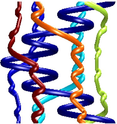
Figure 1: The braid formed by the world lines of a rod and several periodic islands in a mixing device.

The analysis of this braid yields important information about the mixing properties of the flow. For instance, it can be shown that if the braid possesses a positive topological entropy, then there must exist a region in the surrounding fluid that exhibits chaotic trajectories. The presence of chaos is a consequence of the topology of the rod motion, and is guaranteed no matter which dynamical equations the fluid obeys, or whether the flow is laminar or turbulent—hence the name topological chaos. It is well-known (Aref 1984) that chaotic trajectories are very good for mixing, especially in very viscous flows where turbulence is nonexistent.

The reasoning for the presence of chaos involves material lines in the fluid, which are lines that are assumed to move with the fluid, in the manner that a nondiffusing blob of dye would. A material line is dragged and stretched by the fluid motion, but it cannot cross the physical rods. Hence, the material line inherits the complexity of the rod motion because it ‘snags’ on the rods.

But physical rods are not necessary for topological chaos. In two dimensions, any particle orbit is an obstacle to material lines (Thiffeault 2005). Periodic orbits have been particularly useful in characterising topological chaos. Perhaps paradoxically, the most appealing periodic orbits for this purpose are regular islands, also known as elliptic regions. Figure 1 shows the motion of a single rod as well as regular islands created in a viscous flow by the motion of the rod. Topologically speaking, there is no difference between the rod and the islands, and the braid shown here has positive topological entropy (Gouillart et al. 2006). This opens up the intriguing possibility of optimising mixing devices by altering the braid formed by the motion of rods and islands.

In this article we propose to (i) Briefly review the important issues for mixing in fluids (§2); (ii) Describe the theory behind braids and topological chaos (§3–§5); and (iii) Apply braid optimisation techniques to real mixing devices (§6). Along the way we will mention open problems, and in §7 we will discuss future avenues for exploration, and where the challenges lie.

2 Stirring and Mixing in Fluids

It comes as a surprise to many that mixing is actually a proper field of study. After all, how much of a mathematical challenge can stirring milk in a teacup present? Well, quite a difficult one, actually! For the particular case of the teacup, stirring creates turbulence, and turbulent flows are usually extremely good at mixing. Turbulence is hard—if not impossible—to understand, so we are already in dangerous territory.

But it gets worse: the teacup is a poor example because there is not much to achieving good mixing: a flick of the wrist will usually suffice. But there are many other situations of practical interest where this is not the case, for various reasons. The basic setting is the same: given some quantity (e.g., milk, temperature, moisture, salt, dye…, usually referred to as the scalar field) that is transported by a fluid (e.g., air or water), how does the concentration of that substance evolve in time? But from there very different questions can arise:

• Does the scalar concentration tend to a constant distribution, and if so, how rapidly?

• Does the scalar eventually fill the entire domain, or are there transport barriers that prevent this?

• How much energy is required to stir the fluid?

For the teacup, the answer to these questions are: yes, fast; yes; and not very much at all. Note that stirring is the mechanical process that moves the fluid, and mixing is the tendency of the scalar field to homogenise. In this paper we shall use the two words interchangeably.

Let us consider two extreme cases that are more challenging than the teacup. First, oceanic flows: the ocean is preferentially heated at the equator; this causes evaporation, which leads to higher salt concentrations. But clearly the ocean is not becoming hotter and saltier at the equator, so there must be a mechanism that redistributes these two scalars over the globe. One candidate is molecular diffusion, which all scalars undergo, but that is utterly negligible—it would take longer than the age of the earth to redistribute the heat and salt in this way. The primary mode of redistribution is by far transport by oceanic currents. In this case the scalars are active rather than passive, since they influence the flow itself because of the different weight of warm, salty water compared to cold, fresh water. But for climate modelling it is crucial to know how fast the global redistribution of heat and salt occurs. The number of effects that play a role is astounding: tides, storms, the Earth’s rotation, coupling to the atmosphere, bottom topography, etc.

At the opposite end of the spectrum, consider lab-on-a-chip applications. In this case, the fluid motion takes place at micrometre scales in grooves etched on the surface of microchips. At these scales, the motion of a fluid like water behaves as a viscous fluid: turbulence is impractical to achieve. In these applications one wants to take a standard laboratory manipulation and reduce it in size so it can be embedded in a small, hand-held device for, say, forensic work. But many applications require mixing: for instance, a DNA sample needs to be mixed with the appropriate reagent. The problem is that the fluid motion is so regular that mixing is very difficult, and the molecular diffusion of DNA is very slow (larger molecules diffuse more slowly, and DNA is very large indeed by molecular standards). This is where chaotic mixing becomes the best option, and the field has undergone a renaissance because of lab-on-a-chip applications (Stone & Kim 2001; Whitesides & Stroock 2001).

It was Hénon (1966) who first realised that steady three-dimensional flows could have chaotic trajectories. This is a counterintuitive result: the flow pattern is not changing in time, but if one starts two particle trajectories close to each other they diverge exponentially, at a rate given by the so-called Lyapunov exponent of the flow. Aref (1984) realised the same thing for two-dimensional flows with time dependence, and also saw the advantage of this for fluid mixing, coining the term chaotic advection. If the flow is chaotic, it means that fluid particles rapidly become uncorrelated and forget about each other’s whereabouts. But that is exactly what it means for a scalar to be mixed: the initial concentration field is forgotten. In essence, chaotic advection (also called chaotic mixing when diffusion is implicitly assumed to act) can potentially achieve the same result as turbulence as far as mixing is concerned, but with much simpler fluid motion and at a lower energy cost.

A quantity that is closely related to the Lyapunov exponent is the line-stretching exponent: it gives the asymptotic growth rate of material lines. It is always greater than or equal to the Lyapunov exponent, and the mismatch between the two is a measure of the nonuniformity of stretching in the flow. In two-dimensional smooth flows the line-stretching exponent, maximised over all possible initial material lines, is equal to the topological entropy of the flow (Bowen 1978; Franks & Handel 1988; Newhouse & Pignataro 1993). In this paper we will use the topological entropy as a measure of mixing quality, but many other measures are available (Finn et al. 2004).

Here we will be concerned with time-dependent two-dimensional fluid motions, as in Aref (1984). The main application we have in mind is to batch stirring devices, where very viscous fluid in a vat is stirred by rods. The motion of such fluid is approximately two-dimensional. We will see that the choice of motion of the rods (and not the speed) is crucial to achieving good mixing.

3 A Topological View of Fluid Motion

3.1 Isotopy Classes

Having covered the physical background of mixing in §2, we now turn to a mathematical description of fluid motion. This section follows closely Boyland et al. (2000). We consider the periodic motion of a two-dimensional fluid in some domain $R_{n}$ with $n$ identical stirring rods, as in figure 3 for four rods. The rods undergo some prescribed motion in one cycle and return to their initial configuration, possibly having been permuted.

Fluid elements in $R_{n}$ are dragged along by the rods, and their motion after one period is given by a map $f:R_{n}\rightarrow R_{n}$. We assume this map is a diffeomorphism (smooth with smooth inverse), as is typical of physical situations. In practice, this diffeomorphism is obtained by solving a set of fluid equations, such as the Stokes equations for a viscous fluid or the Navier–Stokes equations when inertia is important. But here we take $f$ to be arbitrary, so that it could represent motions that are far from physical and do not satisfy any particular fluid equations. Rather, we will seek to classify $f$ according to its topological properties, regardless of the type of fluid it arises from.

The topological properties of $f$ are encoded in its isotopy class. Two maps are isotopic if they can be continuously deformed into each other, allowing possibly for rotation of the boundaries. If the fluid is ideal, then rotation of the boundaries is irrelevant. If a map $f$ arises from motions that only involve rotation of the rods or the external boundary, then $f$ is said to be isotopic to the identity. For instance, the journal bearing flow (Aref & Balachandar 1986; Chaiken et al. 1986), consisting of two rotating off-centre cylinders, leads to chaotic fluid motions that are isotopic to the identity ($n=1$ in this case). The set of all maps isotopic to $f$ form its isotopy class.

If $n=0$, $1$, or $2$, then all fluid motions are isotopic to the identity, no matter how the rods are moved. The key insight in Boyland et al. (2000) is that for $n\geq 3$ there are fluid motions not isotopic to the identity. These, we will see, lead to chaotic dynamics that are complex in a profound topological sense–topological chaos.

3.2 The Thurston–Nielsen Classification

Given a diffeomorphism $f$, what possible isotopy classes can it belong to? For two-dimensional compact manifolds, the Thurston–Nielsen classification theorem (Thurston 1988; Fathi et al. 1979) tells us that $f$ is isotopic to $f^{\prime}$, the Thurston–Nielsen representative, where $f^{\prime}$ is one of three types of mapping:

1. finite-order: if $f^{\prime}$ is repeated enough times, the resulting diffeomorphism is the identity;

2. pseudo-Anosov (pA): $f^{\prime}$ stretches the fluid elements by a factor $\lambda>1$, so that repeated application gives exponential stretching; $\lambda$ is called the dilatation of $f^{\prime}$, and $\log\lambda$ is its topological entropy.

3. reducible: $f^{\prime}$ leaves a family of curves invariant, and these curves delimit subregions that are of type 1 or 2.

Note that we have omitted some technical details—see Boyland (1994) for a full exposition. For our purposes, the second of these classes (pA) is most important. Anosov diffeomorphisms are the prototypical chaotic maps: they stretch uniformly everywhere. The most famous example is Arnold’s cat map on the torus (Arnold & Avez 1968). A pseudo-Anosov map allows for a finite number of singularities in the stable and unstable foliations of the map.

Our goal in designing an efficient mixer is now clear: we want to induce a diffeomorphism $f$ that is either isotopic to a pseudo-Anosov map, or splits $R_{n}$ into subregions that include type 2 components. The isotopy stability theorem of Handel (Handel 1985) guarantees that $f$ has dynamics that are at least as complicated as the pA map in its isotopy class. In the next section we will see that specifying isotopy classes is conveniently achieved with braids.

4 Enforcing Chaos with Braids

4.1 Braids Label Isotopy Classes

In §3 we saw that the isotopy class of $f$, a diffeomorphism representing periodic fluid motion, is one of three types. Now we introduce a convenient way to label these isotopy classes—braids. To see intuitively how braids come in, lift the stirrer motions to a three-dimensional space-time plot (the ‘world lines’ of the rods), as in figure 2.

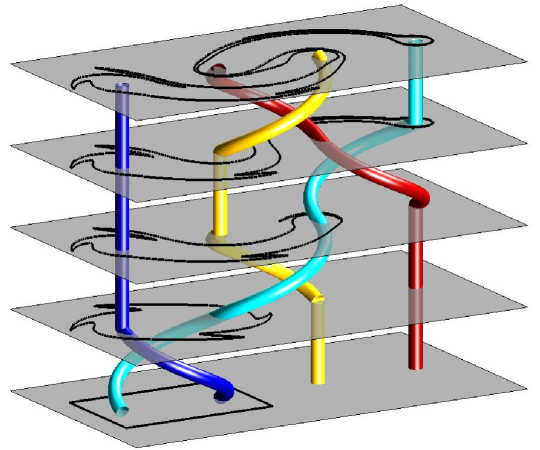
Figure 2: The trajectories of four stirrers define a braid on $n=4$ strands in a space-time diagram, with time flowing from bottom to top. In terms of generators, the braid is written $\sigma_{1}\sigma_{2}^{-1}\sigma_{3}\sigma_{2}^{-1}$, read from left to right. First (bottom) the leftmost two rods are interchanged clockwise ($\sigma_{1}$), then the middle two rods are interchanged counterclockwise ($\sigma_{2}^{-1}$), and so on. The evolution of a material line (black rectangle initially) advected by the flow is also shown.

The resulting plot is called a physical braid. Two braids are equivalent if they can be deformed into each other with no strands crossing other strands or boundaries.

We can pass from physical braids to an algebraic description of braids by introducing generators. Assume without loss of generality that all the stirrers lie on a line. The generator $\sigma_{i}$, $i=1,\ldots,n-1$, denotes the clockwise interchange of the $i$th rod with the $(i+1)$th rod along a circular path, where $i$ is the position of a rod counting from left to right. The counterclockwise interchange is denoted $\sigma_{i}^{-1}$. (See figure 2.) We can write consecutive interchanges as $\sigma_{1}\sigma_{2}^{-1}$, where the generators are read from left to right (this convention differs from Boyland et al. (2000)). This composition law allows us to define the braid group on $n$ strands, $B_{n}$, with the identity given by disentangled strands. In order that braid group elements correspond to physical braids, they must satisfy the additional relations $\sigma_{i}\sigma_{i+1}\sigma_{i}=\sigma_{i+1}\sigma_{i}\sigma_{i+1}$ and $\sigma_{i}\sigma_{j}=\sigma_{j}\sigma_{i}$, for $|i-j|>1$ (Birman 1975).

The crucial role of braids as an organising tool is that they correspond to isotopy classes in $R_{n}$. (There is a subtlety involving possible rotations of the outer boundary, so that one usually speaks of braid types specifying isotopy classes rather than braids (Boyland et al. 2000).) We assign a braid to stirrer motions by the diagrammatic approach employed in figure 2, and to every braid we can assign stirrer motions by reversing the process.

4.2 Good Braids and Bad Braids

So what is to be learned from the braid description of stirrer motions? We can tell directly from the braid which isotopy class the motion belongs to, using the train-track algorithm of Bestvina & Handel (1995). In this paper, we have used a very convenient implementation of this algorithm written by Toby Hall, in which one simply types in the generators, and the program returns the isotopy class and dilatation. We will return to the advantages and disadvantages of the Bestvina–Handel algorithm in §55.2.

In Boyland et al. (2000) as well as subsequent studies (Finn et al. 2003; Vikhansky 2004) a three-rod mixer was considered, as this is the minimum number of rods necessary to guarantee topological chaos. For variety, here we describe a four-rod device, since it has similar properties but has not been described before. In §6 we will see that this device is in some sense as ‘efficient’ as the three-rod device. Figure 3 shows the effect of four stirring rods on a

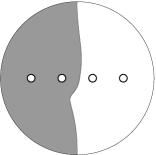
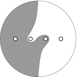
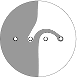
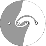
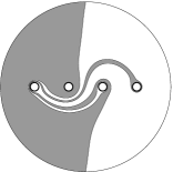
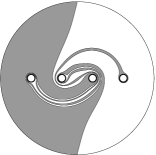
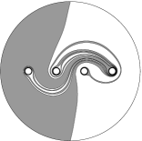
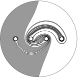
Figure 3: Stirring rods undergoing the braiding motion $\sigma_{1}\sigma_{2}^{-1}\sigma_{3}\sigma_{2}^{-1}$ twice. The generators are read from left to right, and each row is a full cycle of the braid.

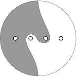
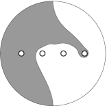
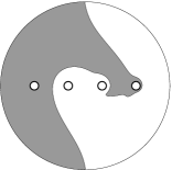
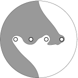
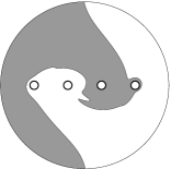
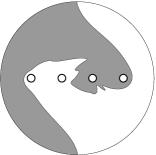
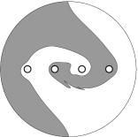
Figure 4: As in figure 3, but for the finite-order braid $\sigma_{1}\sigma_{2}\sigma_{3}\sigma_{2}$.

material line. The rods are undergoing a motion specified by the braid $\sigma_{1}\sigma_{2}^{-1}\sigma_{3}\sigma_{2}^{-1}$, and the flow is viscous Stokes flow. This braid is pA (type 2 in §33.2) with dilatation $\lambda=(7+3\sqrt{5})/2\simeq 6.8541$, which means that, asymptotically in time, a material line must be stretched by at least this factor for every full period of the motion. This is extremely efficient exponential stretching, and we will see in §6 that this particular $\lambda$ is in a sense the optimal efficiency. Figure 3 shows that the diffeomorphism $f$ contains a chaotic type 2 (pA) region, clearly visible as two crescents in the centre, surrounding the rods. It is fair to say that even though the exponential stretching in the region is very large, the mixing region is localised around the stirrers, at least for short times: topological considerations predict nothing about the size of the pA region. In §6 we will return to this issue.

In contrast, figure 4 shows the action of stirring rods moving according to the braid $\sigma_{1}\sigma_{2}\sigma_{3}\sigma_{2}$ on a material line. The length of the line is growing much more slowly, since this braid specifies a finite-order isotopy class. Note that the motions in figure 3 and 4 have the same energetic cost because of symmetry, but the former is far better at mixing.

This suggests that braids that specify pA isotopy classes imply better mixing than finite-order ones. All other things being equal, this is true, but we also see that it is not sufficient: the size of the mixed region in figure 3 is fairly small. In section 6 we will focus on the issue of optimising the braid for best mixing. But first we will see what can be learned from looking at periodic orbits of a flow.

5 Braids as a Diagnosis Tool: Ghost Rods

So far we have looked at producing braids by moving rods in a two-dimensional fluid. The rods, being physical obstacles to material lines, induce a minimum amount of stretching (topological entropy). But any fluid particle orbit is a topological obstacle to material lines. What can we then deduce about the mixing properties of a flow by studying the motion of fluid particles? There are two cases of interest, depending on whether we focus on periodic orbits or chaotic orbits.

5.1 Periodic Orbits

A typical two-dimensional flow will contain chaotic regions and regular islands. The islands are said to be surrounded by a chaotic sea, and for time-periodic flows they are best represented using a stroboscopic map (Poincaré section), which is a snapshot of particle positions at each period of the fluid motion. However, a stroboscopic map hides important information, especially that the islands are moving in between snapshots. In fact, since they form topological obstacles, the islands can be regarded as playing the role of stirring rods. Of course, they are not ‘true’ stirring rods, but we can deduce from their motion important information about the nature of the chaotic sea around the islands. In figure 1 we show the braid formed by regular islands and one stirring rod in a viscous fluid. The topological entropy of this braid is $70\%$ of the measured line-stretching exponent of the chaotic region. (It cannot exceed $100\%$ since it is a lower bound on the line-streching exponent.) In that sense, these islands account for most of the chaos in the region. The rest is accounted for by including unstable periodic orbits in the braid, but these are less useful since they are difficult to measure in practical situations (Gouillart et al. 2006).

Boyland et al. (2003) have also studied periodic braids formed by the motion of point vortices. Since vortices move as fluid particles, they are topological obstacles to material lines. They were thus able to show analytically that chaos must occur. Similarly, Finn et al. (2005) have shown that chaos must occur in the well-known sine flow by following periodic orbits on the torus.

5.2 Chaotic Orbits

Another way to use braids as a diagnosis tool is to measure the braid formed by arbitrary orbits (Thiffeault 2005), periodic, chaotic, or otherwise. The great advantage of this approach is that it can be realised experimentally by sprinkling tracer particles in a flow. The disadvantage is that the meaning of such ‘random’ braids is not on a firm mathematical footing, but the results suggest some interesting directions to pursue (see also Gambaudo & Pécou (1999); Boyland (1994)).

The method is as follows: follow a large number of orbits in a flow, and as they evolve compute the braid associated with their world lines. The braid word recording the crossings becomes longer and longer, but it never repeats if the orbits are not periodic. However, the topological entropy of such a braid appears to converge to a measurable value, in a similar manner to Lyapunov exponents. This topological entropy is a lower bound for the line-stretching exponent of the flow, but the question is how sharp. There are encouraging results that using a large number of particles allows one to measure the topological entropy of a flow fairly accurately (Finn & Thiffeault 2006). This has real practical advantages since the topological entropy is difficult to measure by other means.

Until recently, another difficulty lay in computing the topological entropy for very long braids (with thousands of generators) over many strands. The Burau representation (Kolev 1989) offers an efficient method of computing the entropy, but it only provides a lower bound for more than three strands (and usually not a very good one, as we found in practice). The Bestvina–Handel algorithm mentioned in §44.2 is accurate, but prohibitively expensive even for moderately long braids (forty generators or so). The best new algorithm so far is due to Moussafir (2006): one records the crossings of a curve using coordinates introduced by Dynnikov (2002). The number of crossings yields a sequence that rapidly converges to the topological entropy.

6 Braids as a Design Tool

We have discussed in §4–5 how braids can be used to enforce a minimum amount of stretching in a flow, and how they can be used to diagnose its chaotic properties. Now we turn to a more direct application: can the braiding properties of a set of rods be optimised to give the best possible lower bound on stretching? We will see that, as in many optimisation problems, part of the difficulty lies in formulating the question properly.

6.1 Optimising over Generators

The most basic optimisation problem is this:

What word of length $k$ maximises the entropy in the braid group $B_{n}$?

Clearly, as $k$ gets larger, the maximum entropy also increases since we have more generators to play with. For $n=3$, D’Alessandro et al. (1999) proved that the optimal entropy lies in repeating the word $\sigma_{1}\sigma_{2}^{-1}$ over and over again. The dilatation of this braid is $(3+2\sqrt{5})/2$. This is the square of the Golden ratio $(1+\sqrt{5})/2$, and we refer to the braid $\sigma_{1}\sigma_{2}^{-1}$ as the golden braid. Hence, the entropy per generator of the optimal braid in $B_{3}$ is always equal to the logarithm of the Golden ratio.

What does this mean? The optimal braid arises from a sequence where rods rotate alternately clockwise and counterclockwise. The resulting ‘pile-up’ of material lines can be related to the continued fraction expansion of the Golden ratio, $\{1,1,1,1,\ldots\}$. We also note that the entropy per generator associated with the protocol $\sigma_{1}^{m}\sigma_{2}^{-m}$ is $m^{-1}\log((m+\sqrt{m^{2}+4})/2)$. The argument of the log gives the so-called silver means. These are generalisations of the Golden ratio and have continued fraction representation $\{m,m,m,m,\ldots\}$. As far as we know, this connection between continued fraction expansions and stirring protocols has not been thoroughly investigated. A special case of the silver means, $m=2$, is often called the silver ratio and will be important in §66.2.

Here are some further conjectures about optimal braids. We discovered these by using computer programs to examine large number of braids, but have no rigorous proofs. (Note that Moussafir (2006) has independently formulated these conjectures.) For $n=4$, the braid $\sigma_{1}\sigma_{2}^{-1}\sigma_{3}\sigma_{2}^{-1}$ has entropy per generator equal to the Golden ratio. (This is the ‘good’ braid discussed in §44.2.) It is thus as effective as $\sigma_{1}\sigma_{2}^{-1}$ in $B_{3}$. For $n>5$, all irreducible braids have topological entropy per generator less than the logarithm of the Golden ratio. So the Golden ratio braids only exist for $n=3$ and $4$, and they give the highest possible entropy per generator. Intuitively, these braids involve a tight combination of three or four strands to achieve their high entropy per generator. More strands requires spurious switches down the braid to make it irreducible. A final unproved observation is that the braids with the largest entropy always have alternating signs of noncommuting generators, as in $\sigma_{1}\sigma_{2}^{-1}\sigma_{3}\sigma_{2}^{-1}$.

Note that there is also an optimisation problem for irreducible braids with minimum (but positive) entropy. Paradoxically, the minimum entropy becomes smaller for larger $n$, and it is easy to find sequences of braids that have entropy decreasing as $1/n$. For example, the braid word $\sigma_{1}\sigma_{2}\cdots\sigma_{n-2}\sigma_{2}\sigma_{3}\cdots\sigma_{n-1}$ has entropy approximately equal to $(2/n)\log(2+\sqrt{3})$, for $n$ odd. For $n=5$, this braid has the least entropy of all irreducible braids (Ham & Song 2006). The proof requires a computational train-track automaton, and appears prohibitively difficult for higher $n$. Of course, for our purposes here designing mixers based on the worst braids is not very useful, but it is a mathematically interesting question.

6.2 Silver Mixers

For practical applications, the type of optimisation discussed in §66.1 is fundamentally flawed. The main issue is that the generators of the braid group, $\sigma_{i}$, do not correspond to natural motions of rods in physical systems. For instance, the exchange of the first and last rod in the four-rod system of figure 3 is written $\sigma_{3}\sigma_{1}\sigma_{2}\sigma_{1}\sigma_{3}$ in terms of exchanges of neighbouring rods, so this simple operation requires five generators! But clearly it does not cost much more energy to do this than to exchange the first and second rods ($\sigma_{1}$). The generators do not capture the intrinsic geometry of the system.

Another issue is that motions involving commuting generators (such as $\sigma_{1}$ and $\sigma_{3}$ or any pair of nonadjacent generators) can be performed simultaneously. This is an advantage: energy is not usually the most severe constraint in a real device, so contiguous commuting generators should be weighted as one generator for the purposes of efficiency. Many different optimisation problems can thus be formulated to build in different engineering constraints. In particular, the resulting rod motions must be realisable using a straightforward design.

Here we offer a more specialised approach that obviates these issues. Consider a periodic lattice of two rods, as in figure 5(a). Now perform a $\sigma_{1}$ operation

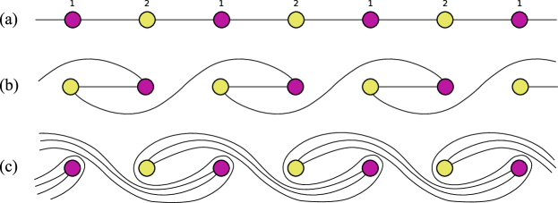
Figure 5: (a) Two rods on a periodic lattice, joined by line segments. The segments are stretched by (b) a clockwise interchange of the rods at positions $1$ and $2$; and (c) a counterclockwise interchange of the rods at position $2$ and $1$.

(figure 5(b)), followed by $\sigma_{2}^{-1}$ (figure 5(c)), where we redefine $\sigma_{2}$ to mean a clockwise interchange of rod $2$ with the next rod to its right, which is the periodic image of rod $1$. It is straightforward to compute the topological entropy per generator of this braid, $\log(1+\sqrt{2})$. The number $1+\sqrt{2}\simeq 2.4142$ is the silver mean for $m=2$ and is called the silver ratio (it is considerably larger than the Golden ratio $(1+\sqrt{5})/2\simeq 1.6180$). For this reason, we refer to the braid $\sigma_{1}\sigma_{2}^{-1}$ for two rods in a periodic lattice as the silver braid. That the silver braid has greater entropy per generator than the golden braid does not contradict the optimality conjecture of §66.1, since that applied to a bounded domain, whereas here we have a periodic array of rods. We have recently examined topological mixing in periodic and biperiodic geometries (Finn et al. 2005; Finn & Thiffeault 2006). A periodic array of two rods is equivalent to arranging an even number of rods in a circle, with a fixed rod in the centre to give the system the topology of an annulus.

The great advantage of this configuration is that it can be implemented practically. Figure 6 shows rod motions that are topologically equivalent

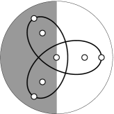
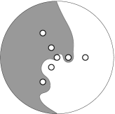
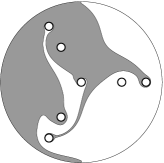
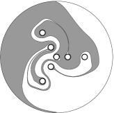
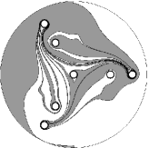
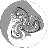
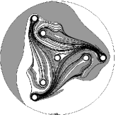
Figure 6: The silver mixing protocol: the central rod and three peripheral rods are fixed, and the other three rods follow the same epicyclic path, shown in the first snapshot.

to the silver braid protocol. The central rod defines the annular domain, and three rods are fixed. The remaining three rods move in an epicyclic motion as shown in the first snapshot. The net effect is that each moving rod executes an ‘over-under’ sequence with the fixed rods as it travels around the mixer, which is exactly the silver braid. As can be seen in the final snapshot, there is a rather large central mixing region where material lines are stretched exponentially fast, at a rate bounded from below by $6\log(1+\sqrt{2})$ for each full cycle, since the rods undergo three $\sigma_{1}\sigma_{2}^{-1}$ exchanges before returning to their initial position. More rods would lead to a greater topological entropy, but would also complicate the apparatus. Of course, topological entropy is not the only important factor: a candidate protocol must also have a reasonably large mixing region, and this can only be deduced by solving fluid equations (viscous Stokes flow here). Figure 6 shows that the silver mixer has a large triangular mixing region, compared for instance with the protocol in figure 3, which has a smaller S-shaped mixing region.

The rod motion in the silver mixer may appear to be quite complicated, and thus difficult to realise, but in figure 7 we show an implementation using Lego™ building blocks.

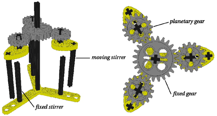
Figure 7: An implementation of the silver mixing protocol in figure 6 using Lego™, drawn with LeoCAD. On the right is a detailed view of the gears.

The central rod supports the whole mechanism, and the three fixed rods are attached to the base. The epicyclic motion of the remaining three rods is realised by having the correct gear ratio (16:24 here). The silver mixer is thus practical from an engineering perspective. By using the result of D’Alessandro et al. (1999), the silver ratio entropy can be shown to be optimal (per generator) for rods arranged in an annulus.

7 The Future

We discuss a few promising areas for future research.

Three-dimensional flows. The most important area of expansion for the type of topological approach presented here is to develop a theory for three-dimensional flows. Knots and braids have been used in three-dimensional flows for a long time, see for instance the book by Ghrist et al. (1997), usually for steady flows. However, three-dimensional applications to mixing analogous to Boyland et al. (2000) are not forthcoming. To some extent, the theory is already three-dimensional, in the sense that if rods extend all the way to the bottom of the mixing device then the braid formed by the rods still gives a bound on the topological entropy. However, this cannot be applied to general orbits. The problem is that lifting three-dimensional particle orbits to a four-dimensional space-time leads to trivial braids. To put it simply, points are not obstacles to lines in three dimensions. Points are obstacles to sheets, and one could imagine trying to record the motion of points as they drag along two-dimensional sheets, but this does not put a lower bound on the area of the sheets. The only option is to follow material lines anchored to the boundary or loops, but so far this has not been very practical and has not been developed.

It was speculated in Boyland et al. (2000) that rods could be inserted in pipe mixers to take advantage of topological effects: the rods would mimic a braid and force the fluid travelling down the pipe to have positive entropy. Finn et al. (2003b) found this to be true, but the chaotic region was tiny and confined near the rods, because of the no-slip boundary condition at rigid surfaces.

Dynamics. Another important area of future exploration is the connection between effective braids and dynamics. We need to understand better the type of situations (geometry, etc.) that yield favorable braiding motions of islands and periodic orbits, as well as produce large, uniform mixing regions. So far the best we can offer are case-by-case analyses, as in Gouillart et al. (2006); Thiffeault et al. (2005), but this is not very satisfactory. In related work, Boyland (2005) has recently investigated the conditions under which Euler’s equation produces time-periodic solutions with pA dynamics.

Open Flows. Most industrial situations involve open flows: fluid enters a mixing region only for a finite time, and then exits, having hopefully been mixed. Can topological considerations tell us anything? The Thurston–Nielsen theorem does not apply, but we can define a topological entropy by looking at the growth rate of material lines or the density of periodic orbits. The braiding motion of unstable periodic orbits (which make up the chaotic saddle) can then be used to put lower bounds on the topological entropy.