Difference in nature of correlation between NASDAQ and BSE indices

Abstract

We apply a recently developed wavelet based approach to characterize the correlation and scaling properties of non-stationary financial time series. This approach is local in nature and it makes use of wavelets from the Daubechies family for detrending purpose. The built-in variable windows in wavelet transform makes this procedure well suited for the non-stationary data. We analyze daily price of NASDAQ composite index for a period of 20 years, and BSE sensex index, over a period of 15 years. It is found that the long-range correlation, as well as fractal behavior for both the stock index values differ from each other significantly. Strong non-statistical long-range correlation is observed in BSE index, whose removal revealed a Gaussian random noise character for the corresponding fluctuation. The NASDAQ index, on the other hand, showed a multifractal behavior with long-range statistical correlation.

1 Introduction

Non-stationary time series have been investigated through several approaches. In particular, the characterization of fluctuations and their scaling behavior have been the focus of many studies, since they reveal the nature of the dynamics. In this context, financial time series have attracted considerable attention Mante . The large length of the available data of various stock market indices make them ideal candidates for analysis. Furthermore, the complex dynamics of the variations in stock prices yield fluctuations which can show correlations, as well as scaling behavior. The goal of the present paper is to study the self-similar and correlation properties of NASDAQ and BSE indices belonging to two different economical environments. These stock indices belonging to developed and developing countries may show characteristic differences, possibly arising due to differences in their underlying dynamics. We concentrate on the nature of correlations and fractal behavior for which wavelet transform daub ; mall is used as a tool for extracting the fluctuations at different scales.

A number of methods have been devised to find scaling behavior in time series. The well-known structure function method ba and the recently developed wavelet transform modulus maxima (WTMM) method arn1 , relying on continuous wavelet transforms, are widely used for the analysis of stationary data. The fact that most of the time series arising in real systems are non-stationary in nature introduces complications in estimating the scaling behavior, while using the above two approaches, which are global in nature. Hence, in recent times, local approaches, like detrended fluctuation analysis (DFA) and its generalization MF-DFA gopi ; muzy ; pen ; khu ; jan have been developed to handle non-stationary data. In this case, one uses windows of various sizes to separate fluctuations from the trend, which can also be shuffled to remove any correlation in the data set. While isolating the average or the trend of the data points in a given window, one takes recourse to linear or quadratic fit in the DFA approach. We have introduced a new method based on discrete wavelets mani1 ; mani2 ; ran to characterize the scaling behavior of non-stationary time series. The present procedure is similar to those in MF-DFA jan , except that in order to detrend, we use wavelets and MF-DFA uses local polynomial fits. Recently, this method has been used by Brodu, to analyze in real time, fractal behavior of dynamic time series nico . The relative merits of MF-DFA and a variety of other approaches to characterize fluctuations have been carried out in Ref.jaro . It is worth emphasizing that fluctuation analysis and characterization have been earlier attempted using Haar wavelets, in the context of bio-medical applications, without the study of scaling behavior pkp1 ; pkp2 .

Wavelets from Daubechies family are used for extracting trend from the given data set. Fluctuations are captured by high-pass coefficients and the trend captured by the low-pass coefficients of wavelet transform. The discrete wavelet transform provide a handy tool for isolating the trend in a non-stationary data set, because of its built-in ability to analyze data in variable window sizes. In this note, we analyze returns of stock index values through our new wavelet based method. Multi-fractal properties are also investigated using multi-fractal spectrum. We analyze daily price of NASDAQ composite index for a period of 20 years, starting from 11-Oct-1984 to 24-Nov-2004, and BSE sensex index, over a period of 15 years, starting from 2-Jan-1991 to 12-May-2005.

2 Data analysis

It is found that the nature of correlation is quite different between these two financial time series and significant non-statistical correlation exists in both of them. Removal of the same reveals that BSE index is primarily mono-fractal with the fluctuations showing a Gaussian random noise character. On the other hand, the NASDAQ index shows a weak multifractal behavior with long range statistical correlation.

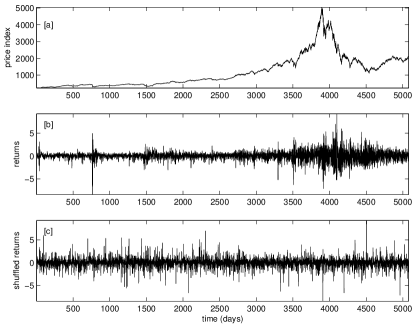
Figure 1: [a] NASDAQ daily (close) composite index for a period of 20 years, starting from 11-Oct-1984 to 24-Nov-2004, [b] daily returns show more clusters of small and large fluctuations and [c] the returns after shuffling show disappearance of clustering behavior.

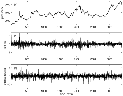
Figure 2: [a] BSE sensex daily (close) index value for a period of 15 years, starting from 2-Jan-1991 to 12-May-2005, [b] daily returns show much less (compared to Fig. 1 (b)) clustering of fluctuations and [c] the returns after shuffling show no significant difference in appearance relative to Fig. 2 (b).

From the financial (NASDAQ composite index and BSE sensex) time series $x(t)$, we first compute the scaled returns defined as,

$$G(t)\equiv[ln(x(t+1))-ln(x(t))]/\sigma,~{}~{}~{}t=1,2...(N-1);$$ (1)

here $\sigma$ is the standard deviation of $x(t)$. From the returns, the signal profile is estimated as the cumulative,

$$Y(i)=\sum_{t=1}^{i}[G(t)],~{}~{}~{}i=1,....,N-1.$$ (2)

Next, we carry out wavelet transform on the profile $Y(i)$ to separate the fluctuations from the trend by considering precise values of window sizes $W$ corresponding to different levels of wavelet decomposition. We obtain the trend by discarding the high-pass coefficients and reconstructing the trend using inverse wavelet transform. The fluctuations are then extracted at each level by subtracting the obtained time series from the original data. Though the Daubechies wavelets extract the fluctuations nicely, its asymmetric nature and wrap around problem affects the precision of the values. This is corrected by applying wavelet transform to the reverse profile, to extract a new set of fluctuations. These fluctuations are then reversed and averaged over the earlier obtained fluctuations. These are the fluctuations (at a particular level), which we consider for analysis. In Figs. 1 and 2, we give the time series for the two index data sets, and the corresponding returns. We also show shuffled returns for the two series to examine the correlation as well as ”bursty” (clustering) behaviour.

The extracted fluctuations are subdivided into non-overlapping segments $M_{s}=int(N/s)$ where $s=2^{(L-1)}W$ is the wavelet window size at a particular level $L$ for the chosen wavelet. Here $W$ is the number of filter coefficients of the discrete wavelet transform basis under consideration. For example, with Db-4 wavelets, $s=4$ at level 1 and $s=8$ at level 2 and so on. It is obvious that some data points would have to be discarded, in case $N/s$ is not an integer. This causes statistical errors in calculating the local variance. In such cases, we have to repeat the above procedure starting from the end and going to the beginning to calculate the local variance. The detrending and extracted fluctuations have been depicted in Figs 3 and 4.

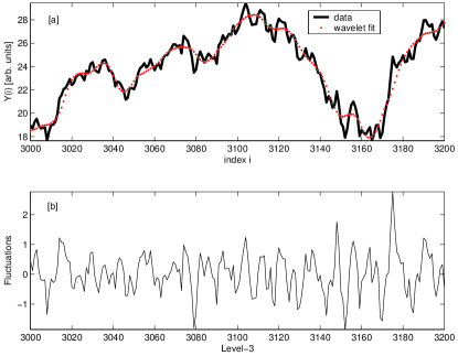
Figure 3: [a] Detrending the integrated returns of NASDAQ composite index at the scale level-3, through Db-8, wavelet, and [b] the extracted fluctuations at the scale level-3 (window size 32).

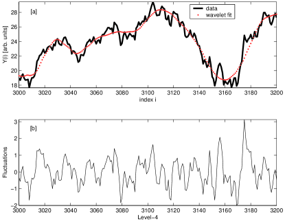
Figure 4: [a] Detrending the integrated returns of NASDAQ composite index at the scale level-4, through Db-8, wavelet, and [b] the extracted fluctuations at the scale level-4 (window size 64).

The $q^{th}$ order fluctuation function $F_{q}(s)$ is obtained by squaring and averaging fluctuations over all segments:

$$F_{q}(s)\equiv\{\frac{1}{2M_{s}}\sum_{b=1}^{2M_{s}}[F^{2}(b,s)]^{q/2}\}^{1/q}.$$ (3)

Here ’$q$’ is the order of moments that takes real values. The above procedure is repeated for variable window sizes for different values of $q$ (except $q=0$). The scaling behaviour is obtained by analyzing the fluctuation function,

$$F_{q}(s)\sim s^{h(q)},$$ (4)

in a logarithmic scale for each value of $q$. If the order $q=0$, direct evaluation through Eq. (3) leads to divergence of the scaling exponent. In that case, logarithmic averaging has to be employed to find the fluctuation function:

$$F_{q}(s)\equiv exp\{\frac{1}{2M_{s}}\sum_{b=1}^{2M_{s}}ln[F^{2}(b,s)]^{q/2}\}^{1/q}.$$ (5)

3 Results and Discussion

As is well-known, if the time series is monofractal, the $h(q)$ values are independent of $q$. For multifractal time series the $h(q)$ values depend on $q$. The correlation behaviour is characterized from the Hurst exponent ($H=h(q=2)$), which varies from $0<H<1$. For long range correlation, $H>0.5$, $H=0.5$ for uncorrelated and $H<0.5$ for long range anti-correlated time series.

The scaling exponent is calculated for various values of $q$ for both the stock index values. Figs. 5 and 6, show the way $h(q)$ and $\tau(q)$ vary with $q$ for the returns and shuffled returns of the two time series. The non-linear behaviour of $h(q)$ for different $q$ values, is the measure of multifractality.

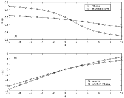
Figure 5: [a](NASDAQ composite index) Scaling exponents h(q) values for various $q$ values and [b] $\tau(q)$ representation of h(q) values for various $q$ values, where $\tau(q)=qh(q)$.

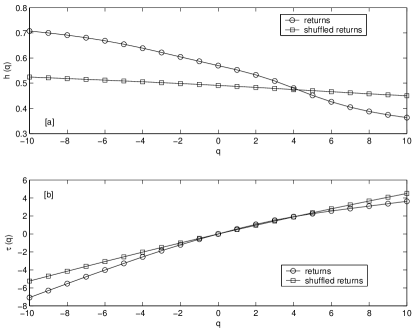
Figure 6: [a] (BSE sensex) Scaling exponents $h(q)$ values for various $q$ values and [b] $\tau(q)$ representation of h(q) values for various $q$ values, where $\tau(q)=qh(q)$.

The scaling behaviour of the observed data sets can also be studied by evaluating $f(\alpha)$ spectrum. $f(\alpha)$ values are obtained from Legendre transform of $\tau(q)$: $f(\alpha)\equiv q\alpha-\tau(q)$, where $\alpha\equiv\frac{d\tau(q)}{dq}$. For monofractal time series, $\alpha=const.$, whereas for multifractal time series there occurs a distribution of $\alpha$ values. The $f(\alpha)$ spectra for the two time series are shown in Figs. 7 and 8. For the unshuffled returns, one observes a broader spectrum, whereas for the shuffled returns, where the correlation is lost, the same is narrower.

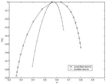
Figure 7: From the integrated returns of NASDAQ composite index values, the calculated multifractal spectrum is broader than the spectrum of shuffled returns.

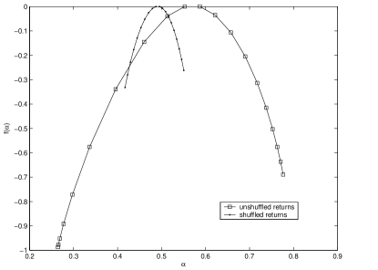
Figure 8: From the integrated returns of BSE sensex values, the calculated multifractal spectrum is much broader than the spectrum of shuffled returns, when compared to the NASDAQ composite index values.

The semi-log plot of distribution of logarithmic returns of NASDAQ composite index values is shown in Fig. 9. It exhibits fat tails and non-Gaussian features. In case of BSE sensex, the semi-log plot of distribution of logarithmic returns shows fat tails, which are less prominent, as shown in Fig. 10. The distribution is quite similar to Gaussian white noise, revealing distinct differences between NASDAQ composite index and BSE sensex values. Although correlation is present in the two time series, they reveal distinct probability distributions once the correlation is removed. Furthermore, we observer that in case of BSE sensex values, the calculated multifractal spectrum is much broader than the spectrum of shuffled returns, when compared to the NASDAQ composite index values.

4 Conclusion

In conclusion, the wavelet based method presented here is found to be quite efficient in extracting fluctuations from trend. It reveals the distinct differences in the long-range correlation, as well as fractal behavior of the two stock index values. Strong non-statistical correlation is observed in BSE index, whereas the NASDAQ index showed a multifractal behavior with long-range statistical correlations. In case of BSE index the removal of correlation revealed the Gaussian random noise character of the fluctuations. It is interesting to note that the effect of country specific parameters like corruption on economic development and investment has been recently quantified through scaling analysis shao . In a similar manner, the above observed differences between the two stock indices belonging to two different economic environment is probably due to local dynamics.

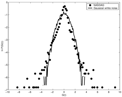
Figure 9: The semi-log plot of distribution of logarithmic returns of NASDAQ composite index values compared with Gaussian distribution.

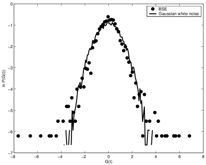
Figure 10: The semi-log plot of distribution of logarithmic returns BSE sensex values compared with Gaussian distribution.

References

- (1) R. N. Mantegna and H. E. Stanley, Introduction to Econophysics: Correlations and Complexity in Finance, Cambridge University Press, Cambridge, 2000.
- (2) Daubechies I., Ten lectures on wavelets SIAM, Philadelphia, 1992.
- (3) S. Mallat, A Wavelet Tour of Signal Processing, 2nd Edition Academic Press, France, 1999.
- (4) P. Gopikrishnan, V. Plerou, L. A. N. Amaral, M. Meyer, and H. E. Stanley, Phys. Rev. E 60 (1999) 5305; K. Matia, Y. Ashkenazy, and H. E. Stanley, Europhys. Lett. 61 (2003) 422; K. Ohashi, L. A. N. Amaral, B. H. Natelson and Y. Yamamoto Phys. Rev. E 68 (2003) 065204(R) .
- (5) J. F. Muzy, E. Bacry and A. Arneodo, Phys. Rev. E 47 (1993) 875.
- (6) C. K. Peng, S. V. Buldyrev, S. Havlin, M. Simons, H. E. Stanley, and A. L. Goldberger, Phys. Rev. E 49 (1994) 1685; R. C. Hwa, C. B. Yang, S. Bershadskii, J. J. Niemela and K. R. Sreenivasan, Phys. Rev. E 72 (2005) 066308.
- (7) B. B. Mandelbrot and J. W. Van Ness, Fractal and Scaling Finance Discontinuity, Concentration, Risk Springer Verlag, New York, 1997.
- (8) A. Arneodo, G. Grasseau, and M. Holshneider, Phys. Rev. Lett. 61 (1988) 2284; J. F. Muzy, E. Bacry, and A. Arneodo, Phys. Rev. E 47 (1993) 875.
- (9) K. Hu, P. Ch. Ivanov, Z. Chen, P. Carpena, and H. E. Stanley, Phys.Rev. E 64 (2001) 11114.
- (10) W. K. Jan, A. Z. Stephen, K. B. Eva, B. Armin, H. Shlomo and H. E. Stanley, Physica A 330 (2003) 240.
- (11) P. Manimaran, P.K. Panigrahi, and J.C. Parikh, Phys. Rev. E 72 (2005) 046120.
- (12) P. Manimaran, P. K. Panigrahi, and J. C. Parikh, eprint: nlin.CD/0601065 (2006).
- (13) P. Manimaran, P. A. Lakshmi and P. K. Panigrahi, J. Phys. A: Math. Gen. 39 (2006) L599.
- (14) N. Brodu, eprint: nlin.CD/0511041 (2005).
- (15) P. Owiecimka, J. Kwapie, and S. Drod, Phys. Rev. E 74 (2006) 016103.
- (16) N. Agarwal, S. Gupta, Bhawna, A. Pradhan, K. Vishwanathan, and P. K. Panigrahi, IEEE J. Sel. Top. Quantum Electron, 9 (2003) 154.
- (17) S. Gupta, M. S. Nair, A. Pradhan, N. C. Biswal, N. Agarwal, A. Agarwal, and P. K. Panigrahi, J. Biomed. Optics 10 (2005) 054012.
- (18) J. Shao, P. Ch. Ivanov, B. Podobnik, and H. Eugene Stanley, Eur. Phys. J. B. 56 (2007) 157.