Abstract

We study the dynamical symmetries of a class of two-dimensional superintegrable systems on a 2-sphere, obtained by a procedure based on the Marsden-Weinstein reduction, by considering its shape-invariant intertwining operators. These are obtained by generalizing the techniques of factorization of one-dimensional systems. We firstly obtain a pair of noncommuting Lie algebras $su(2)$ that originate the algebra $so(4)$. By considering three spherical coordinate systems we get the algebra $u(3)$ that can be enlarged by ‘reflexions’ to $so(6)$. The bounded eigenstates of the Hamiltonian hierarchies are associated to the irreducible unitary representations of these dynamical algebras.

1 Introduction

It is well known that integrable Hamiltonian systems play a fundamental role in the description of physical systems, because their many interesting properties both from mathematical and physical points of view. Many of these Hamiltonian systems have proved to be of an extraordinary physical interest e.g. harmonic oscilator, Kepler problem, Morse [1], Posch–Teller [2], Smorodinski-Winternitz [3, 4], Calogero [5] and Sutherland [6] potentials.

In this paper we present a class of integrable Hamiltonian systems that allow us to generalize the intertwining transformations for one-dimensional (1D) systems [7] to higher dimensions.

These Hamiltonian systems are superintegrable, i.e., they have more than N constants of motion, being N the dimension of the configuration space for the Hamiltonian system. Although these motion integrals are not all of them in involution they determine more than one subset of N constants (in all the cases one of them is the Hamiltonian) in involution. The system is said to be superintegrable in the sense of [8] or maximally superintegrable if there exist $2\,N-1$ invariants well defined in phase–space.

Using the Marsden–Weinstein reduction procedure [9] we construct such classical systems starting from a free Hamiltonian lying in an N-dimensional homogeneous space of a suitable Lie group, whose action allows to us to calculate a momentum map that assure the integrability, or even superintegrability of the reduced systems [4]. From an opposite point of view, there are good reasons to suspect that any integrable system may be constructed as a reduction from a free one [10].

For the corresponding quantum systems we present here a generalization to higher dimensional spaces of the intertwining transformations for 1D factorizable systems. These 1D systems have dynamical Lie algebras of rank one generated by the intertwining operators [7]. By using a concrete superintegrable Hamiltonian system with underlying symmetry the Lie algebra $su(3)$ we find that its dynamical symmetry can bee enlarged to $so(6)$. However, these results can be implemented to higher dimensional systems of the same class, and also can be helpful in the study of other kinds of integrable systems using algebraic methods [11, 12, 13, 14, 15, 16].

In sections 2, 3 and 4 we will introduce a two-dimensional superintegrable system and find some separable solutions by standard procedures (Hamilton-Jacobi equation). Next, in sections 5 and 6 we study the corresponding Schrödinger equation which is factorizable in two 1D equations. We construct some sets of intertwining operators closing the Lie algebras $u(3)$ and $so(6)$ by taking also into account different separable coordinate systems as well as discrete symmetries. We characterize the eigenfunctions of the Hamiltonian hierachies, obtained from the intertwining operators, as irreducible unitary representations of these dynamical algebras.

2 Superintegrable $SU(p,q)$-Hamiltonian systems

Let us consider a free Hamiltonian $H=\,4\,g^{\mu\bar{\nu}}\,p_{\mu}\,\bar{p}_{\nu}$ ($\mu,\nu=0\,,\cdots,n=\,p+q-1$ and the bar stands for complex conjugate) defined in the configuration space $\frac{SU(p,q)}{SU(p-1,q)\times U(1)}$. This is an hermitian hyperbolic space with metric $g_{{\mu}\nu}$ and coordinates $y^{\mu}\in\mathbb{C}$, verifying $g_{\bar{\mu}\nu}\,\bar{y}^{\mu}\,y^{\nu}=\,1$ (by $p_{\mu}$ we denote the conjugate momenta). The geometry and properties of this kind of spaces are described in [17, 18].

Using a maximal abelian subalgebra (MASA) of the Lie algebra $su(p,q)$ [19] the reduction procedure allows us to obtain a reduced Hamiltonian, $H=\,\frac{1}{2}g^{\mu\nu}\,p_{s^{\mu}}\,p_{s^{\nu}}+V(s)$, lying in the corresponding reduced space (a homogeneous $SO(p,q)$-space), where $V(s)$ is a potential depending on the real coordinates $s^{\mu}$ satisfying the constraint $g_{{\mu}\nu}\,{s}^{\mu}\,s^{\nu}=\,1$.

The set of complex coordinates $y^{\mu}$ is transformed by the reduction into a set of ignorable variables $x^{\mu}$ (which are the parameters of the transformation associated to the MASA of $u(p,q)$ used in the reduction) and the actual real coordinates $s^{\mu}$.

If $Y_{\mu}\,,\mu=\,0,\cdots,n$, is a basis of the considered MASA of $u(p,q)$, formed by pure imaginary matrices (this is a basic hypotesis in our reduction procedure), the relation between old ($y^{\mu}$) and new coordinates ($x^{\mu}\,,s^{\mu}$) is

$$y^{\mu}=\,B(x)^{\mu}_{\,\nu}\,s^{\nu}\,,\qquad B(x)=\,\text{exp}\left(x^{\mu}\,Y_{\mu}\right)\,.$$

This relationship assures the ignorability of the $x$ coordinates (the vector fields corresponding to the MASA are straightened out in these coordinates). The Jacobian matrix, $J$, of the coordinate transformation is given explicitly by

$$J=\,\frac{\partial(y\,,\bar{y})}{\partial(x\,,s)}=\,\begin{pmatrix}A&B\\ \bar{A}&\bar{B}\end{pmatrix}\,,\qquad A_{\,\nu}^{\mu}=\,\frac{\partial y^{\mu}}{\partial x^{\nu}}=\,\left(Y_{\nu}\right)^{\mu}_{\,\rho}\,y^{\rho}\,.$$

The Hamiltonian calculated in the new coordinates is written as

$$H=\,c\,\left(\frac{1}{2}\,g^{\mu\,\nu}p_{\mu}\,p_{\nu}+V(s)\right)\,,\qquad V(s)=\,p_{x}^{T}\,(A^{\dagger}\,K\,A)^{-1}\,p_{x}\,,$$

where $p_{x}$ are the constant momenta associated to the ignorable coordinates $x$ and $K$ is the matrix defined by the metric $g$. A detailed exposition of this construction procedure of this family of superintegrable systems can be found in [20].

3 A classical superintegrable $u(3)$-Hamiltonian system

To obtain the classical superintegrable Hamiltonian associated to the unitary Lie algebra $su(3)$ using the reduction procedure sketched in the previous section we are going to proceed in the following way [21].

Let us consider the basis of $su(3)$ determined by $3\times 3$ matrices $X_{1}\,,\cdots,X_{8}$, whose explicit form, when using the metric $K=\text{diag}(1,1,1)$, is

$$X_{1}= \begin{pmatrix}i&0&0\\ 0&-i&0\\ 0&0&0\end{pmatrix} \quad X_{2}= \begin{pmatrix}0&0&0\\ 0&i&0\\ 0&0&-i\end{pmatrix} \quad X_{3}= \begin{pmatrix}0&1&0\\ -1&0&0\\ 0&0&0\end{pmatrix} \quad X_{4}= \begin{pmatrix}0&i&0\\ i&0&0\\ 0&0&0\end{pmatrix}$$

$$X_{5}= \begin{pmatrix}0&0&1\\ 0&0&0\\ -1&0&0\end{pmatrix} \quad X_{6}= \begin{pmatrix}0&0&i\\ 0&0&0\\ i&0&0\end{pmatrix} \quad X_{7}= \begin{pmatrix}0&0&0\\ 0&0&1\\ 0&-1&0\end{pmatrix} \quad X_{8}= \begin{pmatrix}0&0&0\\ 0&0&i\\ 0&i&0\end{pmatrix}\,.$$

In the compact case, as here with $su(3)$, there is only one MASA. This is the Cartan subalgebra, generated by the matrices ${\rm diag}(i,-i,0)$ and ${\rm diag}(0,i,-i)$. However, we shall work, in order to facilitate the computations, with the algebra $u(3)$ instead of $su(3)$. Hence, we shall use the following basis for the corresponding MASA in $u(3)$

$$Y_{0}={\rm diag}(i,0,0),\qquad Y_{1}={\rm diag}(0,i,0),\qquad Y_{2}={\rm diag}(0,0,i).$$

The actual real coordinates $s$ are related to the complex coordinates $y$ by $y_{\mu}=\,s_{\mu}\,e^{i\,x_{\mu}}\;(\mu=0,1,2)$. The Hamiltonian can be written as

$$H=\,\frac{1}{2}\left(p_{0}^{2}+p_{1}^{2}+p_{2}^{2}\right)+V(s)\,,\qquad V(s)=\,\frac{m_{0}^{2}}{s_{0}^{2}}+\frac{m_{1}^{2}}{s_{1}^{2}}+\frac{m_{2}^{2}}{s_{2}^{2}}\,,$$ (3.1)

lying in the 2-sphere $(s_{0})^{2}+(s_{1})^{2}+(s_{2})^{2}=1$.

To see that the system, so obtained, is superintegrable it is necessary to construct its invariants of motion. In this case we obtain three invariants

$$R_{\mu\nu}=\,(s_{\mu}\,p_{\nu}-s_{\nu}\,p_{\mu})^{2}+\left(m_{\mu}\frac{s_{\nu}}{s_{\mu}}+m_{\nu}\,\frac{s_{\mu}}{s_{\nu}}\,\right)^{2},\qquad\mu<\nu,\;\mu=0,1,\;\nu=1,2.$$ (3.2)

Note that only two of them are in involution at the same time (being one of them the Hamiltonian), so the system is superintegrable in the sense of [8]. The sum of these invariants is the Hamiltonian up to an additive constant.

4 The Hamilton-Jacobi equation for the $u(3)$-system

The solutions of the motion problem for this system can be obtained solving the corresponding Hamilton–Jacobi (HJ) equation in an appropriate coordinate system, such that the Hamilton–Jacobi equation separates into a system of ordinary differential equations.

The 2-sphere can be parametrized on spherical coordinates $(\phi_{1},\phi_{2})$ around the $s_{2}$ axis [18, 22] by

$$s_{0}=\cos\phi_{2}\,\cos\phi_{1},\qquad s_{1}=\cos\phi_{2}\,\sin\phi_{1},\qquad s_{2}\,=\sin\phi_{2}$$ (4.1)

where $\phi_{1}\in[0,2\pi)$ and $\phi_{2}\in[\pi/2,3\pi/2]$. Then, the Hamiltonian (3.1) is written as

$$H= \,\frac{1}{2}\,\left(p_{\phi_{2}}^{2}+\frac{p_{\phi_{1}}^{2}}{\cos^{2}\phi_{2}}\right)+V(\phi_{1},\phi_{2}),$$

$$V(\phi_{1},\phi_{2})= \,\frac{1}{\cos^{2}\phi_{2}}\,\left(\frac{m_{0}^{2}}{\cos^{2}\phi_{1}}+\frac{m_{1}^{2}}{\sin^{2}\phi_{1}}\right)+\frac{m_{2}^{2}}{\sin^{2}\phi_{2}}\,.$$

The potential is periodic and has singularities along the coordinate lines $\phi_{1}=0,\pi/2,\pi,3\pi/2$, and $\phi_{2}=\pi/2,3\pi/2$, and thre is a unique minimum inside each regularity domain.

The invariants (3.2) (denoted by $\hat{I}$) can be written in terms of the basis $\{X_{1}\,,\cdots\,,X_{8}\}$ as $\hat{I}_{1}=\,X_{3}^{2}+X_{4}^{2}\,,\hat{I}_{2}=\,X_{5}^{2}+X_{6}^{2}$ and $\hat{I}_{3}=\,X_{7}^{2}+X_{8}^{2}$. The $u(3)$-Casimir is

$$C=\,4\,X_{1}^{2}+2\,\{X_{1}\,,X_{2}\}+4\,X_{2}^{2}+3\,\hat{I}_{1}+3\,\hat{I}_{2}+3\,\hat{I}_{3}\,,$$

where the three first terms are the second order operators in the enveloping algebra of the compact Cartan subalgebra of $u(3)$.

The Hamiltonian is rewritten as $H=\,I_{1}+I_{2}+I_{3}+\text{constant}$, where by $I_{i}$ we denote the invariant $\hat{I}_{i}$ but rewritten in spherical coordinates. So, we have

$$I_{1}= \,\frac{1}{2}\,p_{\phi_{1}}^{2}+\frac{m_{0}^{2}}{\cos^{2}\phi_{1}}+\frac{m_{1}2}{\sin^{2}\phi_{1}},$$

$$I_{2}= \,\tan^{2}\phi_{2}\,\left(\frac{1}{2}p_{\phi_{1}}^{2}\,\sin^{2}\phi_{1}+\frac{m_{0}^{2}}{\cos^{2}\phi_{1}}\right)+\cos^{2}\phi_{1}\,\left(\frac{1}{2}\,p_{\phi_{2}}^{2}+\frac{m_{2}^{2}}{\tan^{2}\phi_{2}}\right)$$

$$\qquad+\,\frac{1}{2}\,p_{\phi_{1}}\,p_{\phi_{2}}\,\sin 2\,\phi_{1}\,\tan\phi_{2},$$

$$I_{3}= \,\tan^{2}\phi_{2}\,\left(\frac{1}{2}p_{\phi_{1}}^{2}\,\cos^{2}\phi_{1}+\frac{m_{1}^{2}}{\sin^{2}\phi_{1}}\right)+\sin^{2}\phi_{1}\,\left(\frac{1}{2}\,p_{\phi_{2}}^{2}+\frac{m_{2}^{2}}{\tan^{2}\phi_{2}}\right)$$

$$\qquad-\frac{1}{2}\,p_{\phi_{1}}\,p_{\phi_{2}}\,\sin 2\,\phi_{1}\,\tan\phi_{2}.$$

Now, the HJ equation takes the form

$${1\over 2}\left({\partial S\over\partial\phi_{2}}\right)^{2}+{m_{2}^{2}\over\sin^{2}\phi_{2}}+{1\over\cos^{2}\phi_{2}}\left({1\over 2}\left({\partial S\over\partial\phi_{1}}\right)^{2}+{m_{0}^{2}\over\cos^{2}\phi_{1}}+{m_{1}^{2}\over\sin^{2}\phi_{1}}\right)=E.$$

It separates into two ordinary differential equations taking into account that the solution of the HJ equation can be written as $S(\phi_{1},\phi_{2})=S_{1}(\phi_{1})+S_{2}(\phi_{2})-Et$. Thus,

$${1\over 2}\left({\partial S_{1}\over\partial\phi_{1}}\right)^{2}+{m_{0}^{2}\over\cos^{2}\phi_{1}}+{m_{1}^{2}\over\sin^{2}\phi_{1}} = \alpha_{1},$$

$${1\over 2}\left({\partial S_{2}\over\partial\phi_{2}}\right)^{2}+{m_{2}^{2}\over\sin^{2}\phi_{2}}+{\alpha_{1}\over\cos^{2}\phi_{2}} = \alpha_{2},$$

where $\alpha_{2}=E$ and $\alpha_{1}$ are the separation constants (which are positive). Each one of these two equations have the same form of those corresponding to the 1D problem [21].

The solutions of both HJ equations are easily computed and can be found as particular cases in Ref. [18]. A detailed analysis of them shows that all the orbits in a neighborhood of a critical point (center) are closed and thus, the corresponding trajectories are periodic (a direct consequence of the correspondence between extrema of the potential and critical points of the phase space).

The explicit solutions, when we restrict us to the domain $0<\phi_{1},\phi_{2}<\pi/2$, are

$$\cos^{2}\phi_{2} = {1\over 2E}\left[b_{2}+\sqrt{b_{2}^{2}-4\alpha_{1}E}\cos 2\sqrt{2E}t\right],$$

$$\cos^{2}\phi_{1} = {1\over 2\alpha_{1}}\left[b_{1}+{1\over\cos^{2}\phi_{2}}\left[{b_{1}^{2}-4\alpha_{1}m_{0}^{2}\over b_{2}^{2}-4\alpha_{1}E}\right]^{1/2}\left((b_{2}\cos^{2}\phi_{2}-2\alpha_{1})\sin 2\sqrt{2\alpha_{1}}\beta_{1}\right.\right.$$

$$\quad\left.\left.+2\sqrt{\alpha_{1}}[(b_{2}-E\cos^{2}\phi_{2})\cos^{2}\phi_{2}-\alpha_{1}]^{1/2}\cos 2\sqrt{2\alpha_{1}}\beta_{1}\right)\right],$$

where $b_{1}=\alpha_{1}+m_{0}^{2}-m_{1}^{2}$ and $b_{2}=E+\alpha_{1}-m_{2}^{2}$.

Note that in this domain for the variables $(\phi_{1},\phi_{2})$ the minimum for the potential corresponds to the point $(\phi_{1}=\arctan\sqrt{m_{1}/m_{0}},\;\phi_{2}=\arctan\sqrt{m_{2}/(m_{0}+m_{1}))}$. The value of the potential at this point is $(m_{0}+m_{1}+m_{2})^{2}$. Hence, the energy $E$ is bounded from below, i.e. $E\geq(m_{0}+m_{1}+m_{2})^{2}$.

As we mentioned before these results reflect essentially the (1D) $su(2)$-case. In fact, all systems we can construct using Cartan subalgebras can be described in a unified way as it was shown in [18, 20, 21].

5 A quantum superintegrable $u(3)$-Hamiltonian system

From the quantum point of view the Hamiltonian (3.1) takes the form

$$H=-\left(J_{0}^{2}+J_{1}^{2}+J_{2}^{2}\right)+\frac{l_{0}^{2}-1/4}{(s_{0})^{2}}+\frac{l_{1}^{2}-1/4}{(s_{1})^{2}}+\frac{l_{2}^{2}-1/4}{(s_{2})^{2}},$$ (5.1)

where $(l_{0},l_{1},l_{2})\in\mbox{\extra R}^{3}$, and $J_{i}=-\epsilon_{ijk}s_{j}\partial_{k}$.

Also in the quantum case, the eigenvalue problem $H\,\Phi=E\,\Phi$ after substituting the coordinates (4.1), takes the form of a separable differential equation

$$\left[-\partial_{\phi_{2}}^{2}+\tan(\phi_{2})\partial_{\phi_{2}}+\frac{l_{2}^{2}{-}1/4}{\sin^{2}(\phi_{2})}+\frac{1}{\cos^{2}(\phi_{2})}\left(-\partial_{\phi_{1}}^{2}+\frac{l_{0}^{2}{-}1/4}{\cos^{2}(\phi_{1})}+\frac{l_{1}^{2}{-}1/4}{\sin^{2}(\phi_{1})}\right)\right]\Phi=E\,\Phi.$$ (5.2)

Taking the solutions separated in the variables $\phi_{1}$ and $\phi_{2}$ as ${\bf\Phi}(\phi_{1},\phi_{2})=f(\phi_{1})g(\phi_{2})$ after replacing in (5.2) we get the equations

$$\left[-\partial_{\phi_{1}}^{2}+\frac{l_{0}^{2}-1/4}{\cos^{2}(\phi_{1})}+\frac{l_{1}^{2}-1/4}{\sin^{2}(\phi_{1})}\right]f(\phi_{1})=\alpha\,f(\phi_{1}),$$ (5.3)

$$\left[-\partial_{\phi_{2}}^{2}+\tan(\phi_{2})\partial_{\phi_{2}}+\frac{\alpha}{\cos^{2}(\phi_{2})}+\frac{l_{2}^{2}-1/4}{\sin^{2}(\phi_{2})}\right]g(\phi_{2})=E\,g(\phi_{2})\,,$$ (5.4)

where $\alpha$ is a separating constant.

These two (one-variable dependent) equations can be solved using the standard factorizations obtaining polynomial solutions. Notice that the results obtained for the first equation will match in a certain way with those of the second one giving rise to degenerate levels.

5.1 The factorization of the $\phi_{1}$-equation

The 1D Hamiltonian corresponding to the equation (5.3) in the variable $\phi_{1}$ can be factorized using the theory of factorizations by Infeld and Hull [7].

The second order differential operator at the l.h.s. of equation (5.3) can be written as a product of first order operators

$$H_{(0)}^{\phi_{1}}=A^{+}_{0}\,A^{-}_{0}+\lambda_{0},$$

where $A_{0}^{\pm}=\,\pm\partial_{\phi_{1}}-(l_{0}+1/2)\,\tan\phi_{1}+(l_{1}+1/2)\,\cot\phi_{1}$, and $\lambda_{0}\,=(l_{0}+l_{1}+1)^{2}$. Also it is possible to construct a family of operators $\{A_{m}^{+},A_{m}^{-}\,,\lambda_{m}\,,H_{(m)}^{\phi_{1}}\}$, $m\in\mbox{\extra Z}$, where

$$A_{m}^{\pm}=\pm\partial_{\phi_{1}}-(l_{0}+m+1/2)\,\tan\phi_{1}+(l_{1}+m+1/2)\,\cot\phi_{1},$$ (5.5)

$$\lambda_{m}=(l_{0}+l_{1}+2\,m+1)^{2},$$

$$H_{(m)}^{\phi_{1}}=-\partial_{\phi_{1}}^{2}+\frac{(l_{0}+m)^{2}-1/4}{{\cos}^{2}\phi_{1}}+\frac{\,(l_{1}+m)^{2}-1/4}{{\sin}^{2}\phi_{1}}\,.$$ (5.6)

Hence, we obtain a 1D Hamiltonian hierarchy (5.6), whose first element is $H_{(0)}^{\phi_{1}}$, satisfies

$$H_{(m)}^{\phi_{1}}=A^{+}_{m}\,A^{-}_{m}+\lambda_{m}=A^{-}_{m-1}\,A^{+}_{m-1}+\lambda_{m-1}.$$ (5.7)

From it we see that the operators $A_{m}^{\pm}$ are shape invariant intertwining operators, i.e.

$$A^{-}_{m}H_{(m)}^{\phi_{1}}=H_{(m+1)}^{\phi_{1}}A^{-}_{m}\ ,\qquad A^{+}_{m}H_{(m+1)}^{\phi_{1}}=H_{(m)}^{\phi_{1}}A^{+}_{m}.$$ (5.8)

Formally, the operators $A^{\pm}_{m}$ acting on a Hamiltonian eigenfunction give another eigenfunction of a consecutive Hamiltonian in the hierarchy with the same eigenvalue, i.e.

$$A^{-}_{m}:{\cal H}_{m}^{\phi_{1}}\to{\cal H}_{m+1}^{\phi_{1}},\qquad A^{+}_{m}:{\cal H}_{m+1}^{\phi_{1}}\to{\cal H}_{m}^{\phi_{1}}.$$

where ${\cal H}_{m}^{\phi_{1}}$ is the eigenfunction space of $H_{(m)}^{\phi_{1}}$ .

The discrete spectrum and the physical eigenstates of $H_{(0)}^{\phi_{1}}$ may be obtained, in principle, from the fundamental states $f_{(m)}^{0}$ (and their eigenvalues) of all the Hamiltonians of the hierarchy $\{H_{(m)}^{\phi_{1}}\}$. The fundamental states are determined by the equation $A^{-}_{m}\,f^{0}_{(m)}=0$ whose solutions, up to a normalization constant, are

$$f^{0}_{(m)}(\phi_{1})=\cos^{l_{0}+m+1/2}(\phi_{1})\,\sin^{l_{1}+m+1/2}(\phi_{1})\,,$$ (5.9)

with eigenvalues $\lambda_{m}=(l_{0}+l_{1}+2\,m+1)^{2}$.

The excited eigenfunction $f_{(0)}^{m}$ of $H_{(m)}^{\phi_{1}}$ can be obtained from the ground eigenstate $f_{(m)}^{0}$ of $H_{(0)}^{\phi_{1}}$ (both with the same eigenvalue) applying consecutive operators $A^{+}$

$$\begin{array}[]{lll}f_{(0)}^{m}&=&A^{+}_{0}\,A^{+}_{1}\cdots A^{+}_{m-1}\,f_{(m)}^{0}\\[8.5359pt] &=&\,N\,\sin^{l_{1}+1/2}(\phi_{1})\,\,\cos^{l_{0}+1/2}(\phi_{1})\,\,P_{m}^{(l_{1},l_{0})}[\cos(2\,\phi_{1})],\end{array}$$ (5.10)

where $P_{n}^{(a,b)}(x)$ are Jacobi polynomials and $N$ a normalization constant. The spectrum of the Hamiltonian $H_{(0)}^{\phi_{1}}$ (5.3) is given by

$$\alpha=\lambda_{m}=(l_{0}+l_{1}+2\,m+1)^{2},\qquad m\in\mbox{\extra Z}^{\geq 0}\ .$$ (5.11)

5.2 The dynamical algebras associated to the $\phi_{1}$-factorization

The shape invariant intertwining operators for the 1D Hamiltonian hierarchy $\{H_{(m)}^{\phi_{1}}\}$ determine some Lie algebras that we can characterize as follows.

Let us define free-index operators $A^{\pm}$ acting inside the total space $\oplus_{m}{\cal H}_{m}$ from the above $A^{\pm}_{(m)}$ by [23, 24]

$$\begin{array}[]{l}A^{+}f_{(m+1)}:=\frac{1}{2}A^{+}_{m}f_{(m+1)}\propto\tilde{f}_{(m)}\\[8.5359pt] A^{-}f_{(m)}:=\frac{1}{2}A^{-}_{m}f_{(m)}\propto\tilde{f}_{(m+1)}\\[8.5359pt] A\,f_{(m)}:=-\frac{1}{2}(l_{0}{+}l_{1}{+}2m)f_{(m)}\propto f_{(m)}\end{array}$$ (5.12)

where $f_{(m)}$ (or $\tilde{f}_{(m)}$) denotes an eigenfunction of $H_{(m)}$. We can rewrite (5.7) as

$$[A,A^{\pm}]=\pm A^{\pm},\qquad[A^{-},A^{+}]=-2A$$ (5.13)

assuming that the action is on any $f_{(m)}$. These commutators determine a Lie algebra $su(2)$ whose Casimir element is ${\cal C}=A^{+}A^{-}+A(A-1)$.

It can be proved (for more details see Ref. [25]) that the eigenstates of the Hamiltonians $H^{\phi_{1}}_{(m)}$ (5.9) can be characterized, if $l_{0}$ and $l_{1}$ are positive o zero integer numbers, in terms of the vectors of the irreducible unitary representations (IUR) of $su(2)$, labeled by the parameter $j$ such that $2j\in\mbox{\extra Z}^{\geq 0}$. Effectively, the ground states $f_{(m)}^{0}$ of $H^{\phi_{1}}_{(m)}$ are characterized by

$$A^{-}f_{(m)}^{0}=0,\qquad A\,f_{(m)}^{0}=-[(l_{0}+l_{1}+2m)/2]f_{(m)}^{0}.$$ (5.14)

Then, we identify (up to a normalization constant)

$$f_{(m)}^{0}=|j_{m},-j_{m}\rangle,\qquad j_{m}=(l_{0}+l_{1}+2m)/2,$$

where $|j_{,}s\rangle$ denotes the vectors of the IUR $`j^{\prime}$ of $su(2)$.

The excited states of $H^{\phi_{1}}_{(m)}$ are obtained using expression (5.10). So, the eigenstate of the $k$-th excited level of $H^{\phi_{1}}_{(0)}$ is

$$f_{(0)}^{k}\equiv|j_{k}+k,-j_{k}+k\rangle,\qquad j_{k}=(l_{0}+l_{1}+2k)/2,\qquad k=0,1,2\dots$$

Moreover, $H^{\phi_{1}}_{(0)}$ (as well as any $H^{\phi_{1}}_{(m)}$) can be expressed in terms of the $su(2)$-Casimir $\cal C$ acting on such representations by $H^{\phi_{1}}_{(0)}=4({\cal C}+1/4)$. Hence, the eigenvalue equation for any of the excited states can be written as follows

$$\begin{array}[]{lllr}H^{\phi_{1}}_{(0)}f_{(0)}^{k}&\equiv&4({\cal C}+1/4)|j_{0}+k,-j_{0}+k\rangle=4(j_{0}+k+1/2)^{2}|j_{0}+k,-j_{0}+k\rangle&\\[4.30554pt] &=&(l_{0}+l_{1}+2k+1)^{2}f_{(0)}^{k},&k=0,1,2,\dots\end{array}$$

However, there is an ambiguity due that different fundamental states (5.9) with values of $l_{0}$ and $l_{1}$ giving the same $j_{0}=(l_{0}+l_{1})/2$ would lead to the same $j_{0}$-representation of $su(2)$.

Adding the diagonal operator $D$, $Df_{(m)}:=(l_{0}-l_{1})f_{(m)}$, to the generators of $su(2)$ (5.12) we obtain $u(2)$. The eigenstates of the Hamiltonian hierarchy are now completly characterized by the IUR’s of $u(2)$. However, different $u(2)$-IUR’s may give rise to (different) states with the same energy.

On the other hand, the states of the Hamiltonian hierarchies, when $l_{0}$ or $l_{1}$ are not in $\mbox{\extra Z}^{\geq 0}$, correspond to non-unitary representations of $u(2)$, although they and their spectra are also given by formulae (5.9) and (5.11), respectively.

From a classification point of view it will be interesting to construct a new Lie algebra, obviously containing the subalgebra chain $su(3)\subset u(3)$, such that only one of its IUR’s characterizes all the eigenstates in the hierarchy with same energy.

In order to build a such dynamical algebra we need to introduce a a two-subindex notation, in terms of the parameters $(l_{0},l_{1})$, for the intertwining operators. The Hamiltonians $H_{(m)}^{\phi_{1}}$ (5.6) will be denoted by $H_{(l_{0},l_{1})}^{\phi_{1}}$, its eigenfunctions by $f_{(l_{0},l_{1})}$, and the factor operators $A_{0}^{\pm}$ in (5.5) will be rewritten as $A_{(l_{0},l_{1})}^{\pm}$. In this way, relation (5.8) can be expressed as

$$A^{-}_{(l_{0},l_{1})}H_{(l_{0},l_{1})}^{\phi_{1}}=H_{{(l_{0}+1,l_{1}+1)}}^{\phi_{1}}A^{-}_{(l_{0},l_{1})}\ ,\qquad A^{+}_{(l_{0},l_{1})}H_{{(l_{0}+1,l_{1}+1)}}^{\phi_{1}}=H_{{(l_{0},l_{1})}}^{\phi_{1}}A^{+}_{(l_{0},l_{1})}.$$

We can also define the free-subindex operators $A^{\pm},A,D$ as in (5.12).

The fact that each two-parameter Hamiltonian $H_{(l_{0},l_{1})}^{\phi_{1}}$ is invariant under the reflections

$$I_{0}:(l_{0},l_{1})\to(-l_{0},l_{1}),\qquad I_{1}:(l_{0},l_{1})\to(l_{0},-l_{1})$$

originates a second factorization ([27, 28, 29]) via conjugation of the operators $A^{\pm},A,D$,

$$\begin{array}[]{lll}I_{0}A^{\pm}I_{0}=\tilde{A}^{\pm},&I_{0}AI_{0}=\tilde{A},&I_{0}DI_{0}=\tilde{D},\\[8.5359pt] \tilde{I}_{1}A^{\pm}I_{1}=\tilde{A}^{\mp},&I_{1}AI_{1}=-\tilde{A},&I_{1}DI_{1}=-\tilde{D}.\end{array}$$

The explicit form of the new operators is

$$\tilde{A}_{(l_{0},l_{1})}^{\pm}=\pm\partial_{\phi_{1}}+(l_{0}{-}1/2)\,\tan\phi_{1}+(l_{1}+1/2)\,\cot\phi_{1},\qquad\tilde{A}_{(l_{0},l_{1})}=-\frac{1}{2}(-l_{0}{+}l_{1}).$$ (5.15)

These operators $\{\tilde{A},\tilde{A}^{\pm}\}$ close a second Lie algebra ${su}(2)$, denoted $\widetilde{su}(2)$, which commutes with the previous ${su}(2)$. Since, moreover, $D$ and $\tilde{D}$ essentially coincide with $\tilde{A}$ and $A$, respectively, the new dynamical algebra is $su(2)\oplus\widetilde{su}(2)\approx so(4)$.

The action of the $so(4)$-generators on a Hamiltonian $H_{(l_{0},l_{1})}^{\phi_{1}}$ originates a 2D parameter $so(4)$-hierarchy $\{H_{l_{0}-n+m,l_{1}+n+m}\}$, $m,n\in\mbox{\extra Z}$, fixed by the initial values $(l_{0},l_{1})$. Each energy level of this Hamiltonian hierarchy is degenerated and the eigenstates are characterized by $so(4)$-representations.

5.3 The factorization of the $\phi_{2}$-equation

The second equation (5.4) can be also factorized provided that the separation constant $\alpha$ is substituted by the eigenvalues obtained from the $\phi_{1}$-factorization $\alpha=\lambda_{m}=(l_{0}+l_{1}+2m)^{2}$. The Hamiltonian associated to this $\phi_{2}$-equation (5.4) is

$$H_{(0)}^{\phi_{2}}={\displaystyle-\partial_{\phi_{2}}^{2}+\tan(\phi_{2})\partial_{\phi_{2}}+\frac{(l_{0}+l_{1}+2m+1)^{2}}{\cos^{2}(\phi_{2})}+\frac{l_{2}^{2}-1/4}{\sin^{2}(\phi_{2})}}.$$ (5.16)

It can be factorized in terms of two first-order differential operators as $H_{(0)}^{\phi_{2}}=M^{+}_{0}M^{-}_{0}+\mu_{0}$. This Hamiltonian $H_{(0)}^{\phi_{2}}$ is the first element of the Hamiltonian hierarchy $\{H_{(n)}^{\phi_{2}}\},\;n\in\mbox{\extra Z}^{\geq 0}$, in the ${\phi_{2}}$–variable, whose elements can be written as

$$H_{(n)}^{\phi_{2}}=M^{+}_{n}M^{-}_{n}+\mu_{n}=M^{-}_{n-1}M^{+}_{n-1}+\mu_{n-1},$$

$$M_{n}^{\pm}=\pm\partial_{\phi_{2}}-(l_{0}+l_{1}+2(m+1)+n)\tan(\phi_{2})+(l_{2}+n+1/2)\cot(\phi_{2}),$$

$$\mu_{n}=(l_{1}+l_{0}+l_{2}+2n+2m+3/2)(l_{2}+l_{1}+l_{0}+2n+2m+5/2).$$ (5.17)

The energy values $E_{n}$ are given by the factorization constant $\mu_{n}$, i.e. $E=\mu_{n}$. The ground states $g_{(n)}^{0}$ for this hierarchy are

$$g_{(n)}^{0}(\phi_{2})=N\cos(\phi_{2})^{l_{1}+l_{0}+2m+1}\sin(\phi_{2})^{l_{2}+n+1/2}\,.$$

The eigenfunctions $g_{(0)}^{n}$ of the initial Hamiltonian $H_{(0)}^{\phi_{2}}$ (5.16) can be written as

$$g_{(0)}^{n}(\phi_{2})=\cos(\phi_{2})^{l_{1}+l_{0}+2m+1}\sin(\phi_{2})^{l_{2}+1/2}P_{n}^{(l_{2}+1/2,l_{1}+l_{0}+2m+1)}[\cos 2\phi_{2}].$$ (5.18)

The index-free operators $M^{\pm}$, defined in a similar way as $A^{\pm}$ in (5.12), close again a Lie algebra $su(2)$. The eigenfunctions (5.18) are square-integrable, but the $su(2)$-representations are IUR provided that the parameters $l_{0},l_{1},l_{2}$ belong to $\mbox{\extra Z}^{\geq 0}$.

The new factorization leads to a degeneration of the energy levels indicating that the underlying dynamical symmetry could be larger than $so(4)$.

Finally joining both factorizations we obtain the square-integrable eigenfunctions separated in the variables $(\phi_{1},\phi_{2})$ of the Hamiltonian (5.2)

$$\Phi_{m,n}(\phi_{1},\phi_{2})=f^{m}_{(0)}(\phi_{1})\,g^{n}_{(0)}(\phi_{2}),\qquad m,n\in\mbox{\extra Z}^{\geq 0},$$

where $f^{m}_{(0)}(\phi_{1}$ and $g^{n}_{(0)}(\phi_{2})$ are given by the expressions (5.10) and (5.18), respectively. Their corresponding eigenvalues $E_{n,m}$ (5.17) are degenerated for the values of $m$ and $n$ whose sum $m+n$ keeps constant [26] (see Figures 1 and 2).

6 Dynamical symmetries of the $u(3)$-Hamiltonian hierarchy

The spectrum of the $u(3)$-Hamiltonian system (5.1) suggestes a bigger dynamical algebra of the Hamiltonian hierarchy. By introducing three sets of intertwining operators closing an algebra $u(3)$ and using reflexion operators this algebra is enlarged to $so(6)$. These three sets of operators are related with three set of spherical coordinates that we can take in the 2-sphere submerged in a 3D ambient space with cartesian axes $\{s_{0},s_{1},s_{2}\}$. Since the axes $(s_{0},s_{1},s_{2})$ play a symmetric role in the Hamiltonian (5.1), we will take their cyclic rotations to get two other intertwining sets. These two set of spherical coordinates also separate the Hamiltonian (5.1).

         

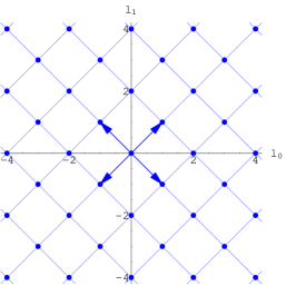
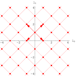
Figure 1: Plot of the two IUR’s $so(4)$-hierarchies, where each point represents a Hamiltonian. At the left it is the integer $(l_{0}=0,l_{1}=0)$ and at the right the half-odd $(l_{0}=0,l_{1}=1)$ hierarchy. The arrows stand for the intertwining operators.

         

Figure 2: The points of the plots represent eigenstates of the underlying half-odd Hamiltonian $so(4)$-hierarchy. At the left, the 4 eigenstates of the $\frac{1}{2}\otimes\frac{1}{2}$ $so(4)$-IUR that share the energy $E=(1+1)^{2}$, and at the right the 16 eigenstates of the $\frac{3}{2}\otimes\frac{3}{2}$ $so(4)$-IUR with $E=(3+1)^{2}$.

6.1 The $u(3)$-Hamiltonian hierarchies

The Hamiltonian as well as the intertwining operators will be labelled now by three parameters $(l_{0},l_{1},l_{2})$ instead of two ones that we made used previously in section 5.2.

The first set of sphere coordinates that we will use is that of coordinates $(\phi_{1},\phi_{2})$ such that the coordinates $\{s_{0},s_{1},s_{2}\}$ are given by (4.1). The Hamiltonian (5.1) characterized by the parameters $\ell\equiv(l_{0},l_{1},l_{2})$ will be now denoted by $H_{(l_{0},l_{1},l_{2})}$, and the operators (5.5) will be rewritten with a three-fold subindex

$$A_{(l_{0},l_{1},l_{2})}^{\pm}=\pm\partial_{\phi_{1}}-(l_{0}+1/2)\,\tan\phi_{1}+(l_{1}+1/2)\,\cot\phi_{1}.$$

The differential operators (5.5) depend only on the variable $\phi_{1}$, hence they do not act on the second separating variable $\phi_{2}$. So, we have the intertwining relations

$$A^{-}_{(l_{0},l_{1},l_{2})}H_{(l_{0},l_{1},l_{2})}=H_{(l_{0}+1,l_{1}+1,l_{2})}A^{-}_{(l_{0},l_{1},l_{2})},\qquad A^{+}_{(l_{0},l_{1},l_{2})}H_{(l_{0}+1,l_{1}+1,l_{2})}=H_{(l_{0},l_{1},l_{2})}A^{+}_{(l_{0},l_{1},l_{2})}.$$

The global operators acting on eigenfunctions of these $H_{(l_{0},l_{1},l_{2})}$ defined as in (5.12),

$$A^{+}\Phi_{(l_{0}+1,l_{1}+1,l_{2})}:=\frac{1}{2}A^{+}_{(l_{0},l_{1},l_{2})}\Phi_{(l_{0}+1,l_{1}+1,l_{2})}\propto\tilde{\Phi}_{(l_{0},l_{1},l_{2})},$$

$$A^{-}\Phi_{(l_{0},l_{1},l_{2})}:=\frac{1}{2}A^{-}_{(l_{0},l_{1},l_{2})}\Phi_{(l_{0},l_{1},l_{2})}\propto\tilde{\Phi}_{(l_{0}+1,l_{1}+1,l_{2})},$$

$$A\,\Phi_{(l_{0},l_{1},l_{2})}:=-\frac{1}{2}(l_{0}+l_{1})\Phi_{(l_{0},l_{1},l_{2})},$$

close an algebra $su(2)$ with commutators like (5.13). Notice that now these operators are acting on the total wavefunction of the complete Hamiltonians like $H_{(l_{0},l_{1},l_{2})}$, not just on a factor function in one-variable.

We will take the spherical coordinates choosing as ‘third axis’ $s_{1}$ instead of $s_{2}$,

$$s_{2}=\cos(\xi_{2})\,\cos(\xi_{1}),\qquad s_{0}=\cos(\xi_{2})\,\sin(\xi_{1}),\qquad s_{1}\,=\sin(\xi_{2})\,.$$

The corresponding intertwining operators $B_{(l_{0},l_{1},l_{2})}^{\pm}$ are defined in a similar way to $A_{(l_{0},l_{1},l_{2})}^{\pm}$. The explicit expressions for the new set in terms of the initial coordinates (4.1) are

$$B_{(l_{0},l_{1},l_{2})}^{\pm}=\pm(\sin\phi_{1}\tan\phi_{2}\partial_{\phi_{1}}+\cos\phi_{1}\partial_{\phi_{2}})-(l_{2}{+}1/2)\,\cos\phi_{1}{\rm cot}\phi_{2}+(l_{0}{+}1/2)\,{\rm sec}\phi_{1}{\rm tan}\phi_{2}.$$

Their intertwining action on the Hamiltonians is

$$B^{-}_{(l_{0},l_{1},l_{2})}H_{(l_{0},l_{1},l_{2})}=H_{(l_{0}+1,l_{1},l_{2}+1)}B^{-}_{(l_{0},l_{1},l_{2})},\qquad B^{+}_{(l_{0},l_{1},l_{2})}H_{(l_{0}+1,l_{1},l_{2}+1)}=H_{(l_{0},l_{1},l_{2})}B^{+}_{(l_{0},l_{1},l_{2})}.$$

The ‘global’ operators, defined by means of multiplicative constant, spann also an algebra $su(2)$.

The spherical coordinates around the $s_{0}$ axis are

$$s_{1}=\cos\theta_{2}\,\cos\theta_{1},\qquad s_{2}=\cos\theta_{2}\,\sin\theta_{1},\qquad s_{0}\,=\sin(\theta_{2}).$$

We obtain a new pair of operators, that written in terms of the original variables $(\phi_{1},\phi_{2})$ are

$$C_{(l_{0},l_{1},l_{2})}^{\pm}=\pm(\cos\phi_{1}\tan\phi_{2}\partial_{\phi_{1}}-\sin\phi_{1}\partial_{\phi_{2}})+(l_{1}{-}1/2)\,{\rm cosec}\phi_{1}{\rm tan}\phi_{2}+(l_{2}{+}1/2)\,{\rm sin}\phi_{1}{\rm cot}\phi_{2}.$$

These operators intertwin the Hamiltonians in the following way

$$C^{-}_{(l_{0},l_{1},l_{2})}H_{(l_{0},l_{1},l_{2})}=H_{(l_{0},l_{1}-1,l_{2}+1)}C^{-}_{(l_{0},l_{1},l_{2})},\qquad C^{+}_{(l_{0},l_{1},l_{2})}H_{(l_{0},l_{1}-1,l_{2}+1)}=H_{(l_{0},l_{1},l_{2})}C^{+}_{(l_{0},l_{1},l_{2})}.$$

The ‘global’ operators (again $1/2$ times the ’old’ ones) close the third $su(2)$.

All these transformations $\{A^{\pm},A,B^{\pm},B,C^{\pm},C\}$ ($C=B-A$) spann an algebra $su(3)$. The $su(3)$-Casimir operator is given by

$${\cal C}=A^{+}A^{-}+B^{+}B^{-}+C^{+}C^{-}+\frac{2}{3}A(A-3/2)+\frac{2}{3}B(B-3/2)+\frac{2}{3}C(C-3/2).$$

We obtain $u(3)$ by adding the central diagonal operator $D:=l_{0}-l_{1}-l_{2}$.

The global operator convention can be adopted for the Hamiltonians $H$ in the $u(3)$-hierarchy by defining its action on the eigenfunctions $\Phi_{(l_{1},l_{2},l_{3})}$ of $H_{(l_{1},l_{2},l_{3})}$ by

$$H\Phi_{(l_{1},l_{2},l_{3})}:=H_{(l_{1},l_{2},l_{3})}\Phi_{(l_{1},l_{2},l_{3})}.$$

Then, the Hamiltonian $H$ can be expressed in terms of both Casimir operators,

$$H=4\,{\cal C}-\frac{1}{3}\,D^{2}+\frac{15}{4}.$$ (6.1)

Hence, the Hamiltonian can be written as a certain quadratic function of the operators $\{A^{\pm},B^{\pm},C^{\pm}\}$ generalizing the usual factorization for 1D systems.

In this way we have built an algebra $u(3)$ of intertwining operators that, once fixed the initial Hamiltonian with parameter values $(l_{0},l_{1},l_{2})$, generate a two-parameter Hamiltonian hierarchy

$$\{H_{(l_{0}+m,l_{1}+m-n,l_{2}+n)}\},\qquad m,n\in\mbox{\extra Z},$$

where the points $(l_{0}+m,l_{1}+m-n,l_{2}+n)$ lie on a certain plane $D=d_{0}$.

One can prove that the eigenstates of this Hamiltonian hierachy are connected to the IUR’s of $u(3)$. Fundamental states $\Phi$ annihilated by $A^{-}$ and $C^{-}$ (simple roots of $su(3)$)

$$A_{\ell}^{-}\Phi_{\ell}=C_{\ell}^{-}\Phi_{\ell}=0$$

only exist when $l_{1}=0$,

$$\Phi_{\ell}(\phi_{1},\phi_{2})=N\,\cos^{l_{0}{+}1/2}(\phi_{1})\sin^{1/2}(\phi_{1})\cos^{l_{0}+1}(\phi_{2})\sin^{l_{2}{+}1/2}(\phi_{2}),$$

whit $N$ a normalizing constant. The diagonal operators act on them as

$$\begin{array}[]{lll}A\,\Phi_{\ell}=-l_{0}/2\,\Phi_{\ell},&l_{0}=m,\qquad l_{1}=0,&m=0,1,2,\dots\\[8.5359pt] C\,\Phi_{\ell}=-l_{2}/2\,\Phi_{\ell},&l_{2}=n,&n=0,1,2,\dots\end{array}$$ (6.2)

This shows that $\Phi_{\ell}$ is the lowest state of the IUR $j_{1}=m/2$ of the subalgebra $su(2)$ generated by $\{A^{\pm},A\}$, and of the IUR $j_{2}=n/2$ of the subalgebra $su(2)$ closed by $\{C^{\pm},C\}$. Such a $su(3)$-representation will be denoted $(m,n)$, $m,n\in\mbox{\extra Z}^{\geq 0}$. The points (labelling the states) of this representation obtained from $\Phi_{\ell}$ lie on the plane $D=m-n$ inside the $\ell$-parameter space.

The energy for the states of the IUR determined by the lowest state (6.2) with parameters $(l_{0},0,l_{2})$, is given (6.1) by

$$E=(l_{0}+l_{2}+3/2)(l_{0}+l_{2}+5/2)=(m+n+3/2)(m+n+5/2).$$ (6.3)

Note that the IUR’s labelled by $(m,n)$ with the same value $m+n$ are associated to states with the same energy. We call such IUR’s a iso-energy series. This degeneration will be broken using the algebra $so(6)$.

6.2 The $so(6)$-hierarchy

Making use of some relevant discrete symmetries, following the procedure of section 5.2, the dynamical algebra $u(3)$ can be enlarged to $so(6)$.

The Hamiltonian $H_{(l_{0},l_{1},l_{2})}$ (5.1) is invariant under reflections in the parameter space $(l_{0},l_{1},l_{2})$

$$I_{0}:(l_{0},l_{1},l_{2})\to(-l_{0},l_{1},l_{2}),\qquad I_{1}:(l_{0},l_{1},l_{2})\to(l_{0},-l_{1},l_{2}),\qquad I_{2}:(l_{0},l_{1},l_{2})\to(l_{0},l_{1},-l_{2})$$

These symmetries, $I_{i}$, can be directly implemented in the eigenfunction space, giving by conjugation another set of intertwining operators (${}_{i}\!X=I_{i}\,X\,I_{i},\;i=0,1,2$) closing an isomorphic Lie algebra ${}_{i}u(3)$. They are (now labelled with a tilde)

$$\begin{array}[]{ll}\{A^{\pm},B^{\pm},C^{\pm}\}\stackrel{{\scriptstyle I_{0}}}{{\longrightarrow}}&\{\tilde{A}^{\mp},\tilde{B}^{\mp},C^{\pm}\},\\[8.61108pt] \{A^{\pm},B^{\pm},C^{\pm}\}\stackrel{{\scriptstyle I_{1}}}{{\longrightarrow}}&\{\tilde{A}^{\pm},B^{\pm},\tilde{C}^{\pm}\},\\[8.61108pt] \{A^{\pm},B^{\pm},C^{\pm}\}\stackrel{{\scriptstyle I_{2}}}{{\longrightarrow}}&\{A^{\pm},\tilde{B}^{\pm},\tilde{C}^{\mp}\}.\end{array}$$

For instance, the sets $\{A^{\pm},A\}$ and $\{\tilde{A}^{\pm},\tilde{A}\}$ close the two commuting $su(2)$ of section 5.2.

The explicit expression for these new intertwining operators can be easily obtained in the same way as was done in (5.15). They close a Lie algebra of rank 3, $so(6)$. Instead of the six non-independent generators $A,\tilde{A},B,\tilde{B},C,\tilde{C}$ it is enough to consider three independent diagonal operators $L_{0},L_{1},L_{2}$ defined by $L_{i}\,\Psi_{(l_{0},l_{1},l_{2})}:=l_{i}\,\Psi_{(l_{0},l_{1},l_{2})}$. The Hamiltonian can be expressed in terms of the $so(6)$-Casimir operator by means of the ‘symmetrization’ of the $u(3)$-Hamiltonian (6.1)

$$H=\{A^{+},A^{-}\}+\{B^{+},B^{-}\}+\{C^{+},C^{-}\}+\{\tilde{A}^{+},\tilde{A}^{-}\}+\{\tilde{B}^{+},\tilde{B}^{-}\}+\{\tilde{C}^{+},\tilde{C}^{-}\}+{L_{0}}^{2}+{L_{1}}^{2}+{L_{2}}^{2}+\frac{41}{12}.$$

The intertwining generators of $so(6)$ give rise to larger 3D Hamiltonian hierarchies

$$\{H_{(l_{0}+m+p,l_{1}+m-n-p,l_{2}+n)}\},\qquad m,n,p\in\mbox{\extra Z},$$

each one including a class of the previous ones coming from $u(3)$. The eigenstates of these $so(6)$-hierarchies can be classified in terms of $so(6)$ representations.

References

- [1] P.M. Morse, Phys. Rev. 34 (1929) 57.
- [2] G. Posch and E. Teller, Z. Phys. 83 (1933) 143.
- [3] P. Winternitz, A. Smorodinsky, M. Uhlir and J. Fris, Soviet J. Nuclear Phys. 4 (1967) 444 .
- [4] N.W. Evans, Phys. Phys. Rev. 41A (1990) 5666; Phys. Lett. 147A (1990) 483; J. Math. Phys. 32 (1991) 3369.
- [5] F. Calogero, J. Math. Phys. 10 (1969) 2191; J. Math. Phys. 10 (1969) 2197.
- [6] B. Sutherland, Phys. Rev. 4A (1971) 2019.
- [7] L. Infeld and T.E. Hull, Rev. Mod. Phys. 23 (1951) 21.
- [8] L.P. Eisenhart, Ann. Math. 35 (1934) 284.
- [9] J. Marsden and A. Weinstein, Rep. Math. Phys. 5 (1974) 121.
- [10] J. Grabowski, G. Landi, G. Marmo and G. Vilasi, Fortschr. Phys. 42 (1996) 393.
- [11] Ş. Kuru, A. Teǧmen and A. Verçin, J. Math. Phys. 42 (2001) 3344.
- [12] B. Demircioǧlu, Ş. Kuru, M. Önder and A. Verçin, J. Math. Phys. 43 (2002) 2133.
- [13] K.A. Samani and M. Zarei, Ann. Phys. 316 (2005) 466.
- [14] M.F. Rañada, J. Math. Phys. 36 (1995) 3541; 38 (1997) 4165; 40 (1999) 236; 41 (2000) 2121.
- [15] M.F. Rañada and M. Santander, J. Math. Phys. 40 (1999) 5026; 43 (2002) 431; 44 (2003) 2149.
- [16] F. Cannata, M.V. Ioffe and D.N. Nishnianidze, J. Phys. A 35 (2002) 1389.
- [17] S. Kobayashi and K. Nomizu, Foundations of Differential Geometry (Wiley, New York, 1969).
- [18] J.A. Calzada, M.A. del Olmo, M.A. Rodríguez, J. Geom. Phys. 23 (1997) 14.
- [19] M.A. del Olmo, M.A. Rodríguez, P. Winternitz and H. Zassenhaus, Linear Algebr. Appl. 135 (1990) 79.
- [20] M.A. del Olmo, M.A. Rodríguez and P. Winternitz, J. Math. Phys. 34 (1993) 5118; Fortschritte der Physik 44 (1996) 91.
- [21] J.A. Calzada, M.A. del Olmo and M.A. Rodríguez, J. Math. Phys. 40 (1999) 88.
- [22] C.P. Boyer, E.G. Kalnins and P. Winternitz, SIAM J. Appl. Math. 16 (1985) 93.
- [23] D.J. Fernández , J. Negro and M.A. del Olmo, Ann. Phys. 252 (1996) 386.
- [24] J. Negro, L.M. Nieto and O. Rosas-Ortiz, J. Phys. A 33 (2000) 7207.
- [25] J.A. Calzada, J. Negro and M.A. del Olmo, “Superintegrable quantum -systems and higher rank factorizations”. math-ph/0601067.
- [26] E.G. Kalnins, W. Miller, G.S. Pogosyan, J. Math. Phys. 37 (1996) 6439.
- [27] A.O. Barut, A. Inomata and R. Wilson, J. Phys. A 20 (1987) 4075; J. Phys. A 20 (1987) 4083.
- [28] A. del Sol Mesa, C. Quesne and Yu F. Smirnov, J. Phys. A 31 (1998) 321.
- [29] M. Dutt, A. Gangopadhyaya, C. Rosinaru and U. Sukhatme, J. Phys. A 34 (2001) 4129.