Polygons for finding exact solutions of nonlinear differential equations

Abstract

New method for finding exact solutions of nonlinear differential equations is presented. It is based on constructing the polygon corresponding to the equation studied. The algorithms of power geometry are used. The method is applied for finding one – parameter exact solutions of the generalized Korteveg – de Vries – Burgers equation, the generalized Kuramoto - Sivashinsky equation, and the fifth – order nonlinear evolution equation. All these nonlinear equations contain the term $u^{m}u_{x}$. New exact solitary waves are found.

Keywords: the simplest equation method, travelling wave, exact solution, power geometry, the Korteveg – de Vries – Burgers equation, the Kuramoto – Sivashinsky equation, nonlinear differential equation.

PACS: 02.30.Hq - Ordinary differential equations

1 Introduction

One of the most important problems of nonlinear models analysis is the construction of their partial solutions. Nowadays this problem is widely discussed. We know that the inverse scattering transform [1, 2, 3] and the Hirota method [4, 3, 5] are very useful in looking for the solutions of exactly solvable nonlinear equations, while most of the nonlinear differential equations describing various processes in physics, biology, economics and other fields of science do not belong to the class of exactly solvable equations.

Certain substitutions containing special functions are usually used for determination of partial solutions of not integrable equations. The most famous algorithms are the following: the singular manifold method [6, 7, 8, 9, 10, 11, 12], the Weierstrass function method [12, 13, 14], the tanh–function method [15, 16, 17, 18, 19, 20], the Jacobian elliptic function method [21, 22, 23], the trigonometric function method [24, 25].

Lately it was made an attempt to generalize most of these methods and as a result the simplest equation method appeared [26, 27]. Two ideas lay in the basis of this method. The first one was to use an equation of lesser order with known general solution for finding exact solutions. The second one was to take into account possible movable singularities of the original equation. Virtually both ideas existed though not evidently in some methods suggested earlier.

However the method introduced in [26, 27] has one essential disadvantage concerning with an indeterminacy of the simplest equation choice. This disadvantage considerably decreases the effectiveness of the method. In this paper we present a new method for finding exact solutions of nonlinear differential equations, which greatly expands the method [26, 27] and which is free from disadvantage mentioned above. When working out our method we used the ideas of power geometry recently developed in [28, 29]. With a help of the power geometry we show that the search of the simplest equation becomes illustrative and effective. Also it is important to mention that the results obtained are sufficiently general and can be applied not only to finding exact solutions but also to constructing transformations for nonlinear differential equations.

The paper outline is as follows. New method for finding exact solution of nonlinear differential equation is introduced in section 2. The application of our approach to the generalized Korteveg – de Vries – Burgers equation is presented in sections 3. Solitary waves of the generalized Kuramoto – Sivashinsky equation and of the nonlinear fifth–order evolution equation are found in sections 4 and 5, accordingly.

2 Method applied

Let us assume that we look for exact solutions of the following nonlinear n-order ODE

$$M_{n}\left(y(z),y_{z}(z),y_{zz}(z),\ldots,z\right)=0.$$ (2.1)

In power geometry any differential equation is regarded as a sum of ordinary and differential monomials. Every monomial can be associated with a point on the plane according to the following rules

$$C_{2}z^{q_{1}}y^{q_{2}}\longrightarrow(q_{1},q_{2}),\,\,\,C_{2}d^{k}y/dz^{k}\longrightarrow(-k,1).$$ (2.2)

Here $C_{1},C_{2}$ are arbitrary constants. When monomials are multiplied their coordinates are added. The set of points corresponding to all monomials of a differential equation forms its carrier. Having connected the points of the carrier into the convex figure we obtain a convex polygon called a polygon of a differential equation. Thus the nonlinear ODE (2.1) is associated with a polygon $L_{1}$ on the plane.

Now let us assume that a solution $y(z)$ of the basic equation can be expressed through solutions $Y(z)$ of another equation. The latter equation is called the simplest equation. Equations having known general solutions or solutions without movable critical points are usually taken as the simplest equations. Consequently we have a relation between $y(z)$ and $Y(z)$

$$y(z)=F(Y(z),Y_{z}(z),\ldots,z).$$ (2.3)

The main problem is to find the simplest equation. Substitution (2.3) into the basic equation (2.1) yields transformed differential equation which is characterized by new polygon $L_{2}$. The suitable simplest equations should be looked for among the equations whose polygons, first, are of lesser or equal area than $L_{2}$ and, second, have all or certain part of edges parallel to those of $L_{2}$. Let us suppose that we have found such polygon $L_{3}$. Then we can write out the simplest equation

$$E_{m}(Y(z),Y_{z}(z),\ldots,z)=0.$$ (2.4)

It is important to mention that the choice of the simplest equation is not unique. If the following relation

$$M_{n}(F(Y,Y_{z},\ldots,z))=\hat{R}\,E_{m}(Y,Y_{z},\ldots,z)$$ (2.5)

(where $\hat{R}$ is a differential operator) is true then it means that for any solution $Y(z)$ of the simplest equation (2.4) there exists a solution of (2.1).

In this paper we will consider a case of identity substitution, i.e.

$$y(z)\equiv Y(z).$$ (2.6)

Then we should study the polygon $L_{1}$ of the equation (2.1) and try to find the polygon $L_{3}$ generated by the simplest equation (2.4). In this case, our method can be subdivided into four steps.

The first step. Construction of the polygon $L_{1}$, which corresponds to the equation studied.

The second step. Construction of the polygon $L_{3}$ which characterizes the simplest equation. This polygon should posses qualities discussed above.

The third step. Selection of the simplest equation with unknown parameters in such a way that it generates the polygon $L_{3}$.

The fourth step. Determination of the unknown parameters in the simplest equation.

To demonstrate our method application let us find exact solutions of nonlinear differential equations belonging to the following class

$$\sum_{k=1}^{n}\,a_{k}\,\frac{d^{k}y(z)}{dz^{k}}-C_{0}\,y(z)+\frac{\alpha}{m+1}\,y^{m+1}(z)=0.$$ (2.7)

This class of nonlinear ordinary differential equations containes a number of differential equations that corresponds to the famous nonlinear evolution equations. They are the Burgers – Huxsley equation, the Korteveg – de Vries – Burgers equation, the Kuramoto – Sivashinsky equation and so on. The following points $M_{1}=(-1,1)$, $M_{2}=(-2,1)$, $\ldots$, $M_{n}=(-n,1)$, $M_{n+1}={(0,1)}$, and $M_{n+2}=(0,m+1)$ are assigned to the monomials of the equations (2.7). The polygon $L_{1}$ corresponding to the equations (2.7) is the triangle presented at figure 1 ((a): $m>0$ and (b): $m<0$).

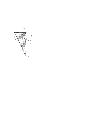
Figure 1: Polygons corresponding to the equations studied and to the simplest equations.

Examining the triangle $L_{1}$ we can easily find the polygon $L_{3}$ assigned to the simplest equation of the first order (see smaller triangles at figure 1). Hence the simplest equation can be written as

$$y_{z}(z)=A\,y^{\frac{n+m}{n}}(z)\,+\,B\,y(z).$$ (2.8)

This equation can be transformed to a linear equation. Its general solution takes the form

$$y(z)\,=\,\left(C_{1}\,\exp{\left\{-\frac{B\,m\,z}{n}\right\}-\,\frac{A}{B}}\right)^{-\frac{n}{m}}.$$ (2.9)

Later, having found the simplest equation, we should determine the coefficients $A$ and $B$ for members of the class (2.7). Then exact solutions of these equations will be expressed through the general solution of the simplest equation.

3 Exact solutions of the generalized Korteveg – de Vries – Burgers equation

Let us find exact solutions of the generalized Korteveg – de Vries – Burgers equation with a help of our method. This equation can be written as

$$u_{t}\,-\alpha\,u^{m}\,u_{x}\,+\,\beta\,u_{xxx}=\nu\,u_{xx}.$$ (3.1)

At $m=1$ and $\nu=0$ (3.1) is the famous Korteveg – de Vries equation. Cauchy problem for this equation is solved by the inverse scattering transform [1]. Soliton solutions of this equation were found using the Hirota method [4]. At $m=1$ and $\nu\neq 0$ a dissipation is taken into account. In this case, the equation (3.1) is not integrable one. Its special solutions were obtained in the work [9]. Later these solutions were rediscovered many times.

Using the travelling wave reduction

$$u(x,t)=y(z),\,\,\,\,\,\,z=x-C_{0}\,t$$ (3.2)

and integrating with respect to $z$, we get

$$\beta\,y_{zz}-\nu\,y_{z}\,-\,C_{0}\,y\,-\,\frac{\alpha}{m+1}\,\,y^{m+1}\,=0,$$ (3.3)

where the constant of integration is equated to zero.

Taking into account the results obtained in section 2, we can write the simplest equation in the form

$$y_{z}(z)=A\,y^{\frac{m+2}{2}}(z)+B\,y(z).$$ (3.4)

The general solution of the equation (3.4) is

$$y{(z)}\,=\,\left(C_{1}\,\exp{\left\{-\frac{B\,m\,z}{2}\right\}-\,\frac{A}{B}}\right)^{-\frac{2}{m}}.$$ (3.5)

Let us formulate our results in the form of the following theorem.

Theorem 3.1.

Let $y(z)$ be a solution of the equation

$$y_{z}(z)\,=\,\pm\,{\frac{\sqrt{2\,\alpha}}{\sqrt{\beta\,({m}+2)(m+1)}}}\,y^{\frac{m+2}{2}}(z)+{\frac{2\,\nu}{\beta\,\left(m+4\right)}}\,y(z)$$ (3.6)

Then there exists a solution of the equation (3.3) that coincides with $y(z)$ provided that $m\neq 0$, $m\neq-1$, $m\neq-2$, $m\neq-4$, and

$$C_{0}\,=-\,\frac{2\,\nu^{2}(m+2)}{\beta\,(m+4)^{2}}.$$ (3.7)

Proof.

Let $M(y,y_{z},y_{zz})=0$ be the generalized Korteveg – de Vries – Burgers equation (3.3). By $E(y,y_{z})=0$ denote the equation (3.6). Substituting

$$y_{z}(z)\,=\,E(y,y_{z})\,+\,A\,y^{\frac{m+2}{2}}(z)\,+B\,y(z)$$ (3.8)

into the equation (3.3) and equating expressions at different powers of $y(z)$ to zero we get algebraic equations for parameters $A$, $B$, and $C_{0}$ in the form

$$\,\beta\,{A}^{2}\left(m+2\right)\left(m+1\right)-2\,\alpha=0,$$ (3.9)

$$\left(m+1\right)\left(\beta\,{B}^{2}-\nu\,B-{\it C_{0}}\right)=0,$$ (3.10)

$$A\left(m+1\right)\left(\beta\,B\,m+4\,\beta\,B-2\,\nu\right)=0.$$ (3.11)

Equations (3.9), (3.10) and (3.11) can be solved and we obtain

$$A_{1,2}=\pm\,{\frac{\sqrt{2\,\alpha}}{\sqrt{\beta\,({m}+2)(m+1)}}},$$ (3.12)

$$C_{{0}}=-B\,\left(\nu-\beta\,B\right),$$ (3.13)

$$B={\frac{2\,\nu}{\beta\,\left(m+4\right)}}.$$ (3.14)

Consequently we have found the parameters $A$, $B$, $C_{0}$ of the theorem and the relation

$$M(y,y_{z},y_{zz})\,=\hat{R}\,E(y,y_{z}),$$ (3.15)

where $\hat{R}$ is a differential operator. ∎

Thus the solution of the equation (3.3) is found. It takes the form

$$y(z)\,=\,\left(\frac{\sqrt{\alpha\,\beta}\,(m+4)}{\sqrt{2\,\nu^{2}\,(m+2)(m+1)}}+C_{1}\,\exp{\left\{-\frac{\nu\,m\,z}{\beta\,(m+4)}\right\}}\right)^{-\frac{2}{m}},$$ (3.16)

where $C_{1}$ is an arbitrary constant.

Note that in the case, $m\rightarrow\,0$ the value of solitary wave velocity (3.7) tends to $C_{0}\,=\,-{(4\,\nu^{2})}/{(16\,\beta)}$, but in the case, $m\rightarrow\infty$ we get $C_{0}\rightarrow\,0$.

It can be shown the correctness of the following formula

$$\left(S_{0}+C_{1}\,\exp{\left\{-\,k\,z\,\right\}}\right)^{-p}\,=\,(2\,S_{0})^{-p}\left(1+\tanh{\left\{\frac{k\,(z+\varphi_{0})}{2}\right\}}\right)^{p},$$ (3.17)

where $S_{0}$ is an arbitrary constant and $\varphi_{0}$ is a constant connected with the coefficient $C_{1}$ by the relation

$$\varphi_{0}=\frac{1}{k}\,\ln{\frac{C_{1}}{S_{0}}}.$$ (3.18)

Using (3.17) the solution (3.16) can be rewritten as

$$y(z)\,=\,\left(\frac{\nu^{2}\,(m+1)(m+2)}{2\,\alpha\,\beta\,(m+4)^{2}}\right)^{\frac{1}{m}}\,\left(1+\tanh{\left\{\frac{\nu\,m\,(z+\varphi_{0})}{2\,\beta\,(m+4)}\right\}}\right)^{\frac{2}{m}}.$$ (3.19)

Assuming $m=1$ in (3.19), we get a solution of the Korteveg – de Vries – Burgers equation in the form

$$y(z)\,=\frac{3\,\nu^{2}}{25\,\alpha\,\beta}\left(1+\tanh{\left\{\frac{\nu\,(z+\varphi_{0})}{10\,\beta\,}\right\}}\right)^{2}.$$ (3.20)

This solution was found in [9].

4 Exact solutions of the generalized Kuramoto – Sivashinsky equation

Let us look for exact solutions of the generalized Kuramoto – Sivashinsky equation, which can be written as

$$\begin{gathered}u_{t}\,+\,\alpha\,u^{m}\,u_{x}\,+\,\delta\,u_{xx}+\,\beta\,u_{xxx}+\,\gamma\,u_{xxxx}\,=\,0.\end{gathered}$$ (4.1)

Equation (4.1) at $m=1$ is the famous Kuramoto – Sivashinsky equation [30, 31], which describes turbulent processes. Exact solutions of the equation (4.1) at $\beta=0$ were first found in [30]. Solitary waves of (4.1) at $\beta\neq 0$ were obtained in [9] and periodical solutions of this equation at $\beta\neq 0$ were first presented in [12].

Using the variables

$$\begin{gathered}x^{\prime}\,=\,x\,\sqrt{\frac{\delta}{\gamma}},\,\,\,\,\,\,t^{\prime}=t\,\frac{\delta^{2}}{\gamma},\,\,\,\,\,\,u^{\prime}=u,\,\,\,\,\,\,\sigma\,=\,\frac{\beta}{\sqrt{\gamma\,\delta}},\,\,\,\,\,\,\alpha^{\prime}\,=\,\frac{\alpha\,\sqrt{\delta\,\gamma}}{\delta^{2}},\end{gathered}$$ (4.2)

we get an equation in the form (the primes are omitted)

$$\begin{gathered}u_{t}\,+\,\alpha\,u^{m}\,u_{x}\,+\,u_{xx}+\,\sigma\,u_{xxx}+\,u_{xxxx}\,=\,0.\end{gathered}$$ (4.3)

Taking into account the travelling wave reduction

$$u(x,t)=y(z),\,\,\,\,\,\,z=x-C_{0}\,t$$ (4.4)

and integrating with respect to $z$, we get the equation

$$y_{zzz}\,+\sigma\,y_{zz}\,+\,y_{z}\,-\,C_{0}\,y\,+\,\frac{\alpha}{m+1}\,\,y^{m+1}\,=0.$$ (4.5)

Here a constant of integration is equated to zero.

In this case, the simplest equation is the following

$$y_{z}=A\,y^{\frac{m+3}{3}}+B\,y,$$ (4.6)

where $A$ and $B$ are parameters to be found.

The general solution of (4.6) takes the form

$$y(z)=\,\left(C_{1}\,\exp{\left\{-\frac{B\,m\,z}{3}\right\}-\,\frac{A}{B}}\right)^{-\frac{3}{m}}.$$ (4.7)

Let us present our result in the following theorem.

Theorem 4.1.

Let $y(z)$ be a solution of the equation

$$y_{z}(z)\,=\left(-\frac{9\,\alpha}{2\,{m}^{3}+11\,{m}^{2}+18\,m+9}\right)^{\frac{1}{3}}\,y^{\frac{m+3}{3}}(z)\,\mp\,{\frac{3}{\sqrt{2\,{m}^{2}+18\,m+27}}}\,\,y(z).$$ (4.8)

Then $y(z)$ is a solution of the equation (4.5) in the case, $m\,\neq\,0$, $m\,\neq\,-1$, $m\,\neq\,-\frac{3}{2}$, $m\,\neq\,-3$, $m\,\neq\,\frac{-9\,\pm\,3\,\sqrt{3}}{2}$, and

$$C_{{0}}=\mp\,{\frac{3\,(2\,{m}^{2}+9\,m+9)}{\left(2\,{m}^{2}+18\,m+27\right)^{3/2}}},\,\,\,\,\,\sigma=\pm\,{\frac{3\,(3+m)}{\sqrt{2\,{m}^{2}+18\,m+27}}}.$$ (4.9)

Proof.

Let $M(y,y_{z},y_{zz})=0$ be the generalized Kuramoto – Sivashinsky equation (4.5). By $E(y,y_{z})=0$ denote the the equation (4.6). Substituting

$$y_{z}(z)\,=\,E(y,y_{z})\,+\,A\,y^{\frac{m+3}{3}}(z)\,+\,B\,y(z)$$ (4.10)

into equation (4.5) and equating coefficients at powers of $y(z)$ to zero, yields algebraic equations for parameters $A$, $B$, $C_{0}$ and $\sigma$ in the form

$${A}^{3}\left(2\,m+3\right)\left(m+3\right)\left(m+1\right)+9\,\alpha=0,$$ (4.11)

$$\left(m+1\right)\left({B}^{3}+\sigma\,{B}^{2}+B-{\it C_{0}}\right)\,=\,0,$$ (4.12)

$${A}^{2}\left(3+m\right)\left(m+1\right)\left(B\,m+3\,B+\sigma\right)=0,$$ (4.13)

$$\left(m+1\right)\left(2\,{\sigma}^{2}{m}^{2}+18\,{\sigma}^{2}\,m\,+\,27\,{\sigma}^{2}\,-\,9\,{m}^{2}\,-\,54\,m\,-\,81\right)=0.$$ (4.14)

Solutions of the equations (4.11), (4.12), (4.13) and (4.14) can be written as

$$\begin{gathered}A_{1}\,=(-9\,\alpha)^{1/3}\,(\,{m}^{3}+11\,{m}^{2}+18\,m+9)^{-1/3},\\ \\ A_{2,3}\,=(-9\,\alpha)^{1/3}\,\left(-\,\frac{1}{2}\,\mp\,i\,\frac{\sqrt{3}}{2}\right)\,\left({m}^{3}+11\,{m}^{2}+18\,m+9\right)^{-1/3},\end{gathered}$$ (4.15)

$$C_{0}\,=\,B\,\left({B}^{2}+\sigma\,B+1\right),\,\,\,\,\,\,\,B\,=-{\frac{\sigma}{3+m}},$$ (4.16)

$$\sigma=\pm\,{\frac{3\,(3+m)}{\sqrt{2\,{m}^{2}+18\,m+27}}}.$$ (4.17)

In final expressions we will take into consideration $A_{1}$ only.

So we have found parameters of the equation (4.7), conditions (4.9), and the relation

$$M(y,y_{z},y_{zz})\,=\hat{R}\,E(y,y_{z}),$$ (4.18)

where $\hat{R}$ is a differential operator. This completes the proof. ∎

The general solution of the equation (4.9) can be presented in the form

$$y(z)\,=\,\left(C+C_{1}\,\exp{\left\{\pm{\frac{\,m\,z}{\sqrt{2\,{m}^{2}+18\,m+27}}}\right\}}\right)^{-\frac{3}{m}},$$ (4.19)

where $C_{1}$ is an arbitrary constant and $C$ is determined by expression

$$C=\,\pm\,{\frac{\sqrt[3]{-9\,\alpha}\,\sqrt{2\,{m}^{2}+18\,m+27}}{3\sqrt[3]{\left(m+3\right)\left(2\,{m}^{2}+5\,m+3\right)}}}.$$ (4.20)

Again we note that the value of solitary wave velocity (4.19) tends to $C_{0}\,=\,\mp\,1/\sqrt{27}$ as $m\rightarrow\,0$, but at the same time $C_{0}\rightarrow\,0$ as $m\rightarrow\infty$.

Assuming $m=1$ in (4.19), we obtain the known solitary wave

$$y(z)=\left(\frac{\sqrt{47}\,\sqrt[3]{-225\,\alpha}}{30}+C_{1}\exp{\left\{\pm{\frac{\,x\,-\,C_{0}\,t}{\sqrt{47}}}\right\}}\right)^{-{3}},\,\,\,C_{0}=\mp\frac{60}{47\sqrt{47}}.$$ (4.21)

and the value of the parameter $\sigma$: $\sigma\,=\,\pm 12/\sqrt{47}$. This solution of the Kuramoto – Sivashinsky equation is the kink [9, 10, 11, 12, 13].

5 Exact solutions of the fifth – order nonlinear evolution equation

Consider the fifth–order nonlinear evolution equation of the form

$$\begin{gathered}u_{t}\,-\alpha\,u^{m}\,u_{x}\,+\,\sigma\,u_{xx}+\,\delta\,u_{xxx}+\,\beta\,u_{xxxx}\,+\,u_{xxxxx}=\,0.\end{gathered}$$ (5.1)

It has the travelling wave solution

$$u(x,t)=y(z),\,\,\,\,\,\,z=x-C_{0}\,t,$$ (5.2)

where $y(z)$ satisfies

$$y_{zzzz}+\beta\,y_{zzz}\,+\delta\,y_{zz}\,+\sigma\,y_{z}\,-\,C_{0}\,y\,-\,\frac{\alpha}{m+1}\,\,y^{m+1}\,=0.$$ (5.3)

Without loss of generality it can be set $\alpha=m+1$. The simplest equation for (5.3) is the following

$$y_{z}(z)=A\,y^{\frac{m+4}{4}}(z)+B\,y(z),$$ (5.4)

where $A$ and $B$ are parameters that should be found.

The general solution of (5.4) is

$$y_{z}=\,=\,\left(C_{1}\,\exp{\left\{-\frac{B\,m\,z}{4}\right\}-\,\frac{A}{B}}\right)^{-\frac{4}{m}}$$ (5.5)

Let us summarize our results in the theorem.

Theorem 5.1.

Let $y(z)$ be a solution of the equation

$$y_{z}(z)\,=\,{\frac{{2}\sqrt[4]{2}}{\sqrt[4]{(m+4)(3m+4)(m+2)}}}\,\,y^{\frac{m+4}{4}}(z)\,-\,{\frac{2\,\beta}{3\,m+8}}\,\,y(z).$$ (5.6)

Then $y(z)$ is also a solution of the equation (5.3) provided that $m\,\neq\,0$, $m\,\neq\,-1$, $m\,\neq\,-\frac{4}{3}$, $m\,\neq\,-2$, $m\,\neq\,-\frac{8}{3}$, $m\,\neq\,-4$, and

$$C_{{0}}\,=\,-{\frac{{\beta}^{4}(m+4)(3m+4)(m+2)}{2\,\left(3\,m+8\right)^{4}}},$$ (5.7)

$$\delta=\,{\frac{{\beta}^{2}\left(11\,{m}^{2}+72\,m+96\right)}{4\,\left(3\,m+8\right)^{2}}},\,\,\,\,\,\,\sigma\,=\,{\frac{{\beta}^{3}\left({m}^{2}+12\,m+16\right)}{4\,\left(3\,m+8\right)^{2}}}.$$ (5.8)

Proof.

Let $M(y,y_{z},y_{zz})=0$ be the equation (5.3). By $E(y,y_{z})=0$ denote the equation (5.6). Substituting

$$y_{z}(z)\,=\,E(y,y_{z})\,+\,A\,y^{\frac{m+4}{4}}(z)\,+\,B\,y(z)$$ (5.9)

into $M(y,y_{z},y_{zz})=0$ and equating expressions at different powers $y(z)$ to zero, we obtain

$${}\,{A}^{4}\left(m+4\right)\left(3\,m+4\right)\left(m+2\right)-32=0,$$ (5.10)

$${C_{0}}-{B}^{4}-\beta\,{B}^{3}-\delta\,{B}^{2}-\sigma\,B=0,$$ (5.11)

$$\left(m+4\right)\left(m+2\right)\left(3\,mB+2\,\beta+8\,B\right)=0,$$ (5.12)

$${}\,\left(m+4\right)\left(7\,{m}^{2}{B}^{2}+48\,m\,{B}^{2}+96\,{B}^{2}+12\,\beta\,m\,B+48\,\beta\,B+16\,\delta\right)=0,$$ (5.13)

$$\begin{gathered}{\frac{9}{64}}\,A\,{m}^{3}{B}^{3}+\frac{9}{4}\,A\,{m}^{2}{B}^{3}+{\frac{27}{2}}\,A\,m\,{B}^{3}+36\,A\,{B}^{3}+{\frac{9}{16}}\,\beta\,A\,{m}^{2}\,{B}^{2}+\\ \\ +{\frac{27}{4}}\,\beta\,A\,m\,{B}^{2}+27\,\beta\,A\,{B}^{2}+\frac{9}{4}\,\delta\,A\,m\,B+18\,\delta\,A\,B+9\,\sigma\,A=0.\end{gathered}$$ (5.14)

Solutions of the equations (5.10), (5.11), (5.12), (5.13), and (5.14) can be written in the form

$$A_{1,2}\,=\,\pm\,{\frac{2\,\sqrt{2}}{\sqrt[4]{2(m+4)(3m+4)(m+2)}}},$$ (5.15)

$$\begin{gathered}A_{3,4}\,=\mp\,{\frac{4}{\sqrt{-2\,\sqrt{2(m+4)(3m+4)(m+2)}}}},\end{gathered}$$ (5.16)

$$C_{{0}}=\beta\,{B}^{3}+\delta\,{B}^{2}+\sigma\,B+{B}^{4},$$ (5.17)

$$B=-\,{\frac{2\,\beta}{3\,m+8}},$$ (5.18)

$$\delta=-{\frac{7}{16}}\,{m}^{2}{B}^{2}-3\,m{B}^{2}-6\,{B}^{2}-\frac{3}{4}\,\beta\,m\,B-3\,\beta\,B,$$ (5.19)

$$\begin{gathered}\sigma=-{\frac{1}{64}}\,{m}^{3}{B}^{3}-\frac{1}{4}\,{m}^{2}\,{B}^{3}-\frac{3}{2}\,m\,{B}^{3}-4\,{B}^{3}-\frac{1}{16}\,\beta\,{m}^{2}\,{B}^{2}-\\ \\ -\frac{3}{4}\,\beta\,m\,{B}^{2}-3\,\beta\,{B}^{2}-\frac{1}{4}\,\delta\,m\,B-2\,\delta\,B.\end{gathered}$$ (5.20)

In final expressions $A_{1},A_{2}$ will be used only.

From obtained expressions (5.17), (5.18), (5.19), and (5.20) we get conditions (5.7), (5.8), and the relation

$$M(y,y_{z},y_{zz})\,=\hat{R}\,E(y,y_{z}),$$ (5.21)

where $\hat{R}$ is a differential operator.

∎

The general solution of (5.6) can be written as

$$y(z)=\left(\pm{\frac{\sqrt[4]{2}\left(3\,m+8\right)}{\sqrt[4]{\beta\,(m+4)(3m+4)(m+2)}}}+C_{1}\exp{\left\{{{{\frac{\beta\,mz}{2(3\,m+8)}}}}\right\}}\right)^{-\frac{4}{m}},$$ (5.22)

where $C_{1}$ is an arbitrary constant.

Let us note that in the case, $m\rightarrow\,0$ the value of solitary wave velocity (5.22) tends to $C_{0}\,=\,-\beta^{2}/256$, but $C_{0}\rightarrow\,0$ as $m\rightarrow\infty$.

6 Conclusion

In this paper a new method to look for exact solutions of nonlinear differential equations is presented. Our goal was to express solutions of equation studied through general solutions of the simplest equations. The basic idea of our approach is to use geometrical representations for nonlinear differential equations. The introduced method allows one to find the suitable simplest equations. Consequently our method is more powerful than many other methods that use an a priori expressions for $y(z)$. In our terminology these methods take the a priori simplest equation. With a help of our approach we have found exact solutions of the following nonlinear differential equations: the generalized Korteveg – de Vries – Burgers equation, the generalized Kuramoto – Sivashinsky equation and nonlinear fifth – order differential equation. All these equations belong to the class (2.7). Finally we would like to mention that this class can be also expanded. Exact solutions of equations belonging to the new class can be constructed with a help of our method.

7 Acknowledgments

This work was supported by the International Science and Technology Center under Project No. B 1213.

References

- [1] C.S. Gardner, J.M. Greene, M.D. Kruskal, R.R. Miura, Phys. Rev. Lett., 19 (1967) 1095 - 1097
- [2] M.J. Ablowitz, D.J. Kaup, A.C. Newell, H. Segur, Phys. Rev. Lett., 31 (1973) 125
- [3] M.J. Ablowitz , P.A. Clarcson , Solitons, Nonlinear Evolution Equations and Inverse Scattering, Cambridge University Press, (1991), 516 p.
- [4] R. Hirota, Phys. Rev. Lett., 27 (1971) 1192 - 1194
- [5] N.A. Kudryashov, Analytical theory of nonlinear differential equations, Institute of Computer Investigations, Moscow-Izhevsk, (2004), 360 p. (in Russian).
- [6] J. Weiss , M. Tabor, G. Carnevalle, J. Math. Phys., 24, (1983), 522
- [7] R. Conte and M. Musette, J. Phys. A.: Math. Gen. 22, (1989), 169-177
- [8] S.R. Choudhary, Phys Lett. A., 159, (1991), 311-317
- [9] N.A. Kudryashov, Journal of Applied Mathematics and Mekhanics, 52, (1988),361-365
- [10] N.A. Kudryashov, Reports of USSR Academy Siences , No.2, 308, (1989), pp. 294 – 298 (in Russian)
- [11] N.A. Kudryashov, Phys Lett. A., 155, (1991), 269 – 275
- [12] N.A. Kudryashov, Phys Lett. A., 147, (1990), 287 – 291
- [13] N.A. Kudryashov, Journal of Applied Mathematics and Mekhanics, 54, (1990), 372-376
- [14] Z.Y. Yan, Chaos, Solitons and Fractals 21, (2004), 1013
- [15] S.Y. Lou, G. Huang, H. Ruan,, J. Phys. A.: Math. Gen., 24, (1991), 587-590
- [16] E.J. Parkes, B.R. Duffy, Computer Physics Communications, 98, (1996), 288-300
- [17] S.A. Elwakil, S.K. El-labany , M.A. Zahran, R. Sabry, Phys. Lett. A., 299, (2002), 179 -188
- [18] E.G. Fan, Phys. Lett. A., 277, 4-5, (2000), 212 – 218
- [19] E.G. Fan, Phys. Lett. A., 282, 1 – 2, (2002), 18 - 22
- [20] N.A. Kudryashov, E.D. Zargaryan,, J. Phys. A. Math. and Gen. 29, (1996), 8067-8077
- [21] G.T. Liu, T.Y. Fan, Phys. Lett. A., 345, (2005), 161-166
- [22] S.K. Liu, Z.T. Fu, S.D. Liu, Q. Zhao, Phys. Lett. A., 289, (2001), 69-74
- [23] Z. Fu, L. Zhang, S. Liu, S. Liu, Phys. Lett. A., 325, (2004), 363 – 369
- [24] Z. Fu, S. Liu, S. Liu, Phys. Lett. A., 326, (2004), 364 – 374
- [25] C. T. Yan, Phys. Lett. A., 224, (1996), 77
- [26] N.A. Kudryashov, Phys Lett. A., 342, (2005), 99 – 106
- [27] N.A. Kudryashov, Chaos, Solitons and Fractals, 24, (2005), 1217 – 1231
- [28] Bruno A.D. Power geometry in algebraic and differential equations, Moscow, Nauka, Fizmatlit, (1998), 288 p (in Russian).
- [29] Bruno A.D. Asimptotics and expansions of solutions of ordinary differential equations, Uspehi of mathematical nauk, v. 59, No. 3, (2004), p. 31-80 (in Russian).
- [30] Y. Kuramoto, T. Tsuzuki, Prog. Theor. Phys., 55, (1976), 356
- [31] G.I. Sivashinsky, Physica D, 4, (1982), 227 – 235