Breathers or quasibreathers?

Abstract

For the James breathers in the $K_{2}-K_{3}-K_{4}$ chain and for breathers in the $K_{4}$-chain, we prove numerically that these dynamical objects are not strictly time-periodic. Indeed, for the both cases, there exist certain deviations in the vibrational frequencies of the individual particles, which certainly exceed the possible numerical errors. We refer to the dynamical objects with such properties as quasibreathers. For the $K_{4}$-chain, a rigorous investigation of existence and stability of the breathers and quasibreathers is presented. In particular, it is proved that they are stable up to a certain strength of the intersite part of the potential with respect to its on-site part. We conjecture that the main results of this paper are also valid in the general case and, therefore, it seems that one must speak about quasibreathers rather than about strictly time-periodic breathers.

I Introduction

According to the conventional definition Aubry ; flach-1 ; Flach-2 , discrete breathers are spatially localized and time-periodic excitations in nonlinear lattices. Because of the space localization, different particles vibrate with essentially different amplitudes. On the other hand, it is typical for nonlinear systems that frequencies depend on amplitudes of vibrating particles. Therefore, it is not obvious how a discrete breather can exist as an exact time-periodic dynamical object because, in this case, the particles with considerably different amplitudes must vibrate with the same frequency. Surprisingly, we did not find an explicit answer to this question in the literature on discrete breathers.

This paper is devoted to some aspects of the above problem. In Sec. II, we consider the breathes introduced by James in Ref. l4 and arrive at the conclusion that there are some deviations of the vibrational frequencies of the individual particles from the average breather frequency and these deviations certainly exceed the possible numerical errors.

On the other hand, the analytical form of the discrete breathers used in l4 ; l5 is not an exact solution to the nonlinear dynamical equations of the $\ K_{2}-K_{3}-K_{4}$ chain and, therefore, one can suspect that the above deviations are induced by an inaccuracy of the initial conditions for solving the appropriate Cauchy problem.

To establish results beyond suspicion, we consider discrete breathers in a nonlinear chain with a uniform on-site and intersite potential of the forth order (see Sec. III). In other words, we study the $\ K_{2}-K_{3}-K_{4}$ chain with $K_{2}=K_{3}=0$ and call it ”$K_{4}$-chain”. For this case, there exists a localized nonlinear normal mode (NNM) by Rosenberg l6 ; l7 which represents an exact discrete breather (DB). Let us note that DBs for such potentials were discussed in a number of papers (see, for example, Refs. l8 ; l9 ), but from a somewhat different point of view. Here, we obtain practically exact form of the DB and study its stability. It turns out that any infinitesimal vicinity of the exact breather solution consists of stable dynamical objects (for the appropriate strength of the intersite potential) which are not time-periodic. The strict periodicity occurs only along a certain line in the space of possible initial conditions which give rise to NNM. All other initial conditions generate the dynamical objects which can be considered as quasibreathers, because they correspond to quasiperiodic motion. As a consequence, there are some deviations in the vibrational frequencies of the individual breather’s particles similar to those for the James breathers.

Since, in every physical or computational experiment, we cannot tune exactly onto a line in the many-dimensional space of all possible initial shapes of the desired periodic solution, it is reasonable to speak only about quasibreathers. It seems that such situation occurs not only for the considered case admitting the exact solution, but also for the general case.

In connection with the above mentioned term ”quasibreathers”, let us note that the term ”quasiperiodic breathers” is used in literature for different dynamical objects (see Conclusion to this paper).

II James breathers

An approximate analytical form of breathers with small amplitudes for the $\ K_{2}-K_{3}-K_{4}$ chain was obtained in l4 . Some computational experiments with these breathers were presented in l5 . The main results of l4 ; l5 can be outlined as follows.

Let us consider a nonlinear chain of $\tilde{N}=2N+1$ identical masses ($m=1$) which are equidistant in the equilibrium state. Interaction only between the nearest neighboring particles is assumed. Then dynamical equation for the $\ K_{2}-K_{3}-K_{4}$ chain reads

$$\ddot{x}_{n}=V^{\prime}(x_{n+1}-x_{n})-V^{\prime}(x_{n}-x_{n-1}),\;\;\;\;n=-N..N,$$ (1)

$$V(u)=K_{2}u^{2}+K_{3}u^{3}+K_{4}u^{4}.$$ (2)

Here $x_{n}$ is a displacement of $n$-th particle from its equilibrium position, $V(u)$ and $V^{\prime}(u)$ are the potential of the interparticle interaction and its derivative, respectively.

It was proved by James that for any $\omega_{b}$ (breather frequency) slightly exceeding the maximal phonon frequency $\omega_{max}$ (in our case, $K_{2}=\frac{1}{2}$ and, therefore, $\omega_{max}=2$), i.e. $\omega_{b}^{2}=4+\mu,\;\;\;\mu\ll 1$ , there exists the following breather solution to Eqs. (1,2):

$$\ y_{n}(t)=(-1)^{n}\sqrt{\frac{2\mu}{B}}\frac{\cos(\omega_{b}t)}{\cosh\left(n\sqrt{\mu}\right)},$$ (3)

where $B=\frac{1}{2}V^{(4)}(0)-(V^{(3)}(0))^{2}$,

$$y_{n}\equiv V^{\prime}(u_{n})=2K_{2}u_{n}+3K_{3}u_{n}^{2}+4K_{4}u_{n}^{3},\;\;\;\;u_{n}=x_{n}-x_{n-1}.$$ (4)

Here $y_{n}$ are new variables introduced instead of the old variables $x_{n}$ (actually these new variables represent forces acting on the particles of the chain).

Thus, Eq. (3) determines a family of breather solutions. Indeed, there exist a breather with amplitude proportional to $\sqrt{\mu}$ for any fixed frequency $\omega_{b}$. The smaller the deviation of the breather frequency $\omega_{b}$ from the maximal phonon frequency 2, the less the amplitude of the breather. For the case $\mu\rightarrow 0$, the hyperbolic cosine in the denominator of (3) goes to unity for all numbers $n$ and, therefore, the breather localization get worse. Actually, in this limit, breather tends to the extended $\pi$-mode with the infinitesimal amplitude .

Computational experiments reported in l5 have confirmed the theoretical breather shape (3). We tried to reproduce some results of that paper, for example, those depicted in Fig. 1. To this end we started with Eq. (3) for $t=0$, solved the cubic equations (4) for obtaining the initial conditions for $x_{n}(t)$, and then integrated numerically the differential equations (1) of the $\ K_{2}-K_{3}-K_{4}$ chain.

Figure 1: Mean square deviation $\eta(t)$ for the James breather for long-time interval. All parameters are the same as in Table 1. Time $t$ is given in periods $T_{0}=\pi$ of the $\pi$-mode.

Using the numerical values of $K_{2}$, $K_{3}$, $K_{4}$, $\omega_{b}$ and other parameters from the paper l5 , we indeed obtained some localized dynamical objects which seemed to be time-periodic at first sight. But a closer examination revealed more complexity.

Bearing in mind the question posed in Introduction, we began to follow the evolution of frequencies of the individual particles participating in the breather vibration. Some results of this analysis are presented below.

In Table 1, we give the frequencies of nine particles ($n=-4..4$) near the center ($n=0$) of the breather which were calculated within certain time intervals close to the instants $t_{k}$ listed in the first row of the table. Note that all these frequencies $\omega_{j}(t_{k})$ are sufficiently close to the breather frequency $\omega_{b}=2.01$, which was used in Eq. (3), but their deviations from $\omega_{b}$ certainly exceed the possible numerical errors.

Let us comment on the computational procedure. We used the fourth-order Runge-Kutta method with time step $h$ of about $0.0003\ T_{0}$, where $T_{0}=\dfrac{2\pi}{\omega_{max}}=\pi.$ For the times given in Table 1, our simulations conserved the total energy of the chain up to $10^{-10}$. The frequencies of the individual particles were obtained by calculating adjacent zeros of the functions $x_{j}(t)$ in certain intervals near fixed instants $t_{k}$. In turn, these zeros were computed by dichotomy and by Newton-Rafson method.

It is expedient to introduce certain mean values characterizing frequency deviations of the individual breather particles. We specify the mean value $\bar{\omega}(t_{k})$ and the mean square deviation $\eta(t_{k})$ of different $\omega_{j}(t_{k})$ for the breather particles at the moment $t_{k}$ as follows:

$$\bar{\omega}(t_{k})=\frac{1}{M}\cdot\sum_{j}\omega_{j}(t_{k}),$$ (5)

$$\eta(t_{k})=\sqrt{\frac{\sum_{j}[\omega_{j}(t_{k})-\bar{\omega}(t_{k})]^{2}}{M(M-1)}}.$$ (6)

Here $j=-M..M\;\;(M<N)$ are numbers of the breather particles with significant values of $x_{j}(t)$. The values $\bar{\omega}(t_{k})$ and $\eta(t_{k})$ are given, respectively, in the two last rows of Table 1. In the last column of this table, we give

$$\sigma_{j}=\sqrt{\frac{\sum_{t_{k}}[\omega_{j}(t_{k})-\bar{\omega}(t_{k})]^{2}}{\tilde{M}(\tilde{M}-1)}}$$ (7)

which represents the mean square deviation of the frequency for each breather particle after averaging upon different moments (for this averaging, we have used all the frequencies $\omega_{j}(t)$ which were calculated up to $t=t_{k}$ indicated it Table 1). [Note that $M$ in Eqs. (5,6) is the number of considered breather particles, while $\tilde{M}$ in Eq. (7) is the number of $\omega_{j}(t)$ which were calculated].

Table 1: Deviations in frequencies of the individual particles for the James breather in $K_{2}-K_{3}-K_{4}$ chain with $\tilde{N}=101$ particles. Here $K_{2}=0.5$, $K_{3}=-0.1$, $K_{4}=0.25$, $\omega_{b}=2.01$, $\mu=0.0401$, $T_{0}=\pi$, $h=0.001$

	$t_{1}=100\,T_{0}$	$t_{2}=600\,T_{0}$	$t_{3}=1000\,T_{0}$	$t_{4}=1500\,T_{0}$	$\sigma$
$\omega_{-4}$	2.0101459926	2.0097251337	2.0109780929	2.0085043104	2.3348301075e-5
$\omega_{-3}$	2.0068349042	2.0093263880	2.0070499430	2.0100257555	2.4686634177e-5
$\omega_{-2}$	2.0112977946	2.0089800520	2.0110369763	2.0080931884	2.6957224898e-5
$\omega_{-1}$	2.0065877923	2.0099366007	2.0070857334	2.0101152322	2.9130307350e-5
$\omega_{0}$	2.0117517055	2.0086968158	2.0110115290	2.0080038280	2.9739839019e-5
$\omega_{1}$	2.0065877923	2.0099366007	2.0070857334	2.0101152322	2.9130307350e-5
$\omega_{2}$	2.0112977946	2.0089800520	2.0110369763	2.0080931884	2.6957224898e-5
$\omega_{3}$	2.0068349042	2.0093263880	2.0070499430	2.0100257555	2.4686634177e-5
$\omega_{4}$	2.0101459926	2.0097251337	2.0109780929	2.0085043104	2.3348301075e-5
$\bar{\omega}$	2.0090538525	2.009403685	2.00925700227051	2.0090534223
$\eta$	7.61439353253e-4	1.5116218526e-4	6.9232221345e-4	3.2690761972e-4

Some questions arise in connection with the result.

1. Because $\eta(t_{k})$ are rather small, one can suspect that they brought about by certain numerical errors. Is it true?

2. Formula (3) represents only an approximation to the unknown exact breather solution since it was obtained by neglecting some higher-order terms l4 ; l5 . To what extent the appearance of nonzero $\eta(t_{k})$ reflects the properties of the real breather?

3. Is there any growth of $\eta(t_{k})$ for large times? It is an important question because such growth, if exists, possibly means the onset of stability loss of the exact breather solution.

To shed some light on numerical errors problem, we computed $\eta(t_{k})$ and $\sigma_{j}$ for the $\pi$-mode which represents a strictly periodic dynamical regime in any nonlinear chain (see, for example, l10 ; l11 ). Using the same computational procedure as that for obtaining Table 1, we get Table 2 for the case of the $\pi$-mode vibrations. From the latter table, one can see that deviations $\eta(t_{k})$ and $\sigma_{j}$ for the $\pi$-mode turn out to be zero (up to machine precision). Comparing these results with those from Table 1, we conclude that deviations in vibrational frequencies of the individual particles for the James breather are not numerical errors.

Table 2: Frequencies of the individual particles for the $\pi$-mode with amplitude $A=0.1$. Here $K_{2}=0.5$, $K_{3}=-0.1$, $K_{4}=0.25$, $T_{0}=\pi$, $h=0.001$

	$100\,T_{0}$	$600\,T_{0}$	$1000\,T_{0}$	$1500\,T_{0}$	$\sigma$
$\omega_{-4}$	2.00748367227	2.00748367227	2.00748367227	2.00748367227	0
$\omega_{-3}$	2.00748367227	2.00748367227	2.00748367227	2.00748367227	0
$\omega_{-2}$	2.00748367227	2.00748367227	2.00748367227	2.00748367227	0
$\omega_{-1}$	2.00748367227	2.00748367227	2.00748367227	2.00748367227	0
$\omega_{0}$	2.00748367227	2.00748367227	2.00748367227	2.00748367227	0
$\omega_{1}$	2.00748367227	2.00748367227	2.00748367227	2.00748367227	0
$\omega_{2}$	2.00748367227	2.00748367227	2.00748367227	2.00748367227	0
$\omega_{3}$	2.00748367227	2.00748367227	2.00748367227	2.00748367227	0
$\omega_{4}$	2.00748367227	2.00748367227	2.00748367227	2.00748367227	0
$\bar{\omega}$	2.00748367227	2.00748367227	2.00748367227	2.00748367227
$\eta$	0	0	0	0

The function $\eta(t)$ is depicted for large time intervals in Fig. 1. This function was found by calculating all zeros of each displacement $x_{j}(t)$ and averaging the obtained frequencies $\omega_{j}(t)$ with the aid of Eq. (6). From this figure, it is obvious that $\eta(t)$ does not increase in magnitude, and demonstrates certain oscillations similar to chaotic.

The above discussed behavior of the breather particles will be interpreted in the next sections with an example of a model which admits an exact breather solution.

III Existence of breathers in the $K_{4}$-chain

We consider $2N+1$ particles chains with fourth-order potential and periodic boundary conditions. The potential includes both on-site and intersite parts. In contrast to the on-site terms, the intensity of the intersite terms will be varied. We write this potential in the form

$$U=\frac{1}{4}\sum_{n}x_{n}^{4}+\frac{\beta}{4}\sum_{n}(x_{n}-x_{n-1})^{4}.$$ (8)

The Newton dynamical equations for such chain can be written as follows:

$$\ddot{x}_{n}=-x_{n}^{3}+\beta[(x_{n+1}-x_{n})^{3}-(x_{n}-x_{n-1})^{3}],\;\;\;\ n=-N..N,$$ (9)

$$x_{N+1}(t)=x_{-N}(t),\;\;\ x_{-N-1}(t)=x_{N}(t).$$ (10)

Here $\beta$ is the parameter characterizing the intensity of the intersite potential. It will be shown that stability of the breather solution in the chain (9) depends essentially on the value of $\beta$ (see below).

Models similar to (9) have been considered in the papers l8 ; l9 , but we analyze the chain (9) with different purposes and in a different manner.

It is well-known that space and time variables can be separated in Eq. (9) and this was done in l8 (for the case without on-site potential). We prefer to treat breather solution to (9) in terms of the nonlinear normal modes (NNM) introduced by Rosenberg in l6 ; l7 . Indeed, it was proved that for any uniform potential there exist (localized or/and delocalized) NNMs which represent strictly periodic motion of all the particles of the considered mechanical system. More precisely, equations of motion of a many particle system for the dynamical regime corresponding to a fixed NNM reduce to only one differential equation for the displacement $x_{0}(t)$ of an arbitrary chosen particle (this is the so called ”leading” or ”governing” equation), while displacements $x_{j}(t)$ $(j\neq 0)$ of all the other particles are proportional to $x_{0}(t)$ at any instant $t$. Such dynamical behaviour is remeniscent of the linear normal modes whose time dependence is represented by sinusoidal functions because the leading equation, in this case, is the equation of the harmonic oscillator.

It is worth to mention that ”bushes of modes” introduced in l12 and investigated in a number of other papers l13 ; l14 ; l15 ; l10 ; l11 represent a quasiperiodic motion because we have $m$ leading differential equations for the $m$-dimensional bush and, therefore, NNMs should be thought of as one-dimensional bushes.

Below, we consider the procedure for obtaining NNMs. Assuming

$$x_{n}(t)=k_{n}x_{0}(t),\;\;\;\ n=-N..N,$$ (11)

for any time $t$ with constant coefficients $k_{n}$ and substituting this expression into Eq. (9), we obtain

$$k_{n}\ddot{x}_{0}=\{-k_{n}^{3}+\beta[(k_{n+1}-k_{n})^{3}-(k_{n}-k_{n-1})^{3}]\}x_{0}^{3},$$ (12)

where

$$k_{N+1}=k_{-N},\;\;\;k_{-N-1}=k_{N}$$ (13)

in accordance with the boundary conditions (10).

The leading equation (it corresponds to $n=0$) reads:

$$\ddot{x}_{0}=\{-1+\beta[(k_{1}-1)^{3}-(1-k_{-1})^{3}]\}x_{0}^{3},$$ (14)

because we can assume $k_{0}=1$.

Demanding all other equations (12) to be identical to Eq. (14), we obtain the following relations between the unknown coefficients $k_{n}$ ($n=-N..N,\ n\neq 0$):

$$-k_{n}^{3}+\beta[(k_{n+1}-k_{n})^{3}-(k_{n}-k_{n-1})^{3}]=k_{n}\{-1+\beta[(k_{1}-1)^{3}-(1-k_{-1})^{3}]\}.$$ (15)

Thus, we arrive at the system of $2N$ algebraic equations with respect to $2N$ unknowns $k_{n}$ (Eqs. (13) must be taken into account).

Any solution to Eq. (15) determines a certain form of NNM or its spatial profile. In our case, there are some localized and delocalized modes among these solutions. In particular, one of the solutions to Eq. (15) represents the $\pi$-mode. Obviously, every localized NNM is an exact discrete breather in accordance with its definition as spatially localized and time-periodic vibration. The time dependence of the breather is determined by the leading equation (14) which can be solved in terms of the Jacobi elliptic function $\mbox{cn}\left(\tau,\frac{1}{\sqrt{2}}\right)$ (see below). Note that this result was obtained in l8 .

In this paper, we will be interested only in the breather solution which is symmetric with respect to its center. Therefore, we must assume the following relation to hold:

$$k_{-n}=k_{n},\;\;\;n=-N..N.$$ (16)

Taking into account Eq. (16) allows us to reduce by a half the number of unknowns in Eq. (15). Let us write down these equations for the cases $N=1$ and $N=2$ in the explicit form.

For N=1, we have the chain with three particles only ($\tilde{N}=3$). In this case, the dynamical equations (9) read:

$$\begin{array}[]{l}\ddot{x}_{-1}=-x_{-1}^{3}+\beta[(x_{0}-x_{-1})^{3}-(x_{-1}-x_{1})^{3}],\\ \ddot{x}_{0}=-x_{0}^{3}+\beta[(x_{1}-x_{0})^{3}-(x_{0}-x_{-1})^{3}],\\ \ddot{x}_{1}=-x_{1}^{3}+\beta[(x_{-1}-x_{1})^{3}-(x_{1}-x_{0})^{3}].\end{array}$$ (17)

According to Eqs. (11) and (16), the symmetric breather pattern ($k_{-1}=k_{1}\equiv k$) reads

$$\{kx_{0}(t),\;x_{0}(t),\;kx_{0}(t)\}.$$ (18)

Substituting this pattern into Eqs. (17), we obtain the following algebraic equation from the condition of identity of all these equations :

$$k(1+k)+\beta(1-k)^{2}(1+2k)=0.$$ (19)

Since the root $k=k(\beta)$ of Eq. (19) is a function of $\beta$, let us choose $\beta=0.3$ (below, it will be shown that the breather is certainly stable for this value of $\beta$).

Using MAPLE, we obtain

$$k=-0.29344944496399996095.$$ (20)

Let us note that calculating all the Rosenberg modes with the aid of Eq. (15) we used the MAPLE specification Digits=20. Nevertheless, some values that have been calculated with such precision will be, for compactness, presented with a smaller number of digits.

Analogously, for the case $N=2$, the chain consists of five particles ($\tilde{N}=5$) and we must search the symmetric breather pattern as follows

$$\{k_{2}x_{0}(t),\;k_{1}x_{0}(t),\;x_{0}(t),\;k_{1}x_{0}(t)\;,k_{2}x_{0}(t)\}.$$ (21)

Then the algebraic equations for $k_{1}$ and $k_{2}$ read

$$\begin{array}[]{lll}k_{1}[-1+2\beta(k_{1}-1)^{3})]=-k_{1}^{3}+\beta[(k_{2}-k_{1})^{3}-(k_{1}-1)^{3}],\\ k_{2}[-1+2\beta(k_{1}-1)^{3}]=-k_{2}^{3}-\beta(k_{2}-k_{1})^{3}\end{array}$$ (22)

and we obtain the following roots of these equations for $\beta=0.3$:

$$\begin{array}[]{lll}k_{1}=-0.29928831163054746768,\\ k_{2}=0.00359934143244973138.\end{array}$$ (23)

Continuing in this manner, we find symmetric breathers for the chains with $\tilde{N}=7,9,11,13,etc$. particles. Some results of these calculations are presented in Table 3. Being calculated with 20 digits, these results are practically the exact breather solutions for the corresponding $K_{4}$ chains. Moreover, comparing the profiles for the chains with $\tilde{N}=9$ and $\tilde{N}=15$ particles, one can reveal that the further increase of $\tilde{N}$ does not affect the spatial profile of the breather solution. Indeed, the considered breathers demonstrate so strong localization that the displacements of the particles distant by more than three lattice spacings from the breather center are utterly insignificant (they don’t exceed $10^{-20}$ and we denote them in the tables by asterisk). Therefore, we conclude that the profile for $\tilde{N}=19$ (and even for $\tilde{N}=5$) can be considered as that for the infinite chain ($\tilde{N}=\infty$).

For the case without the on-site potential we have for $\tilde{N}=3$: $k_{0}=1$, $k_{-1}=k_{1}=-0.5$. The similar results for $\tilde{N}=5,9,15$ are presented in Table 4. From this table, it is obvious that the results of Ref. l8 don’t correspond to the exact solution for the case of the infinite chain since the author has used the profile only for $\tilde{N}=3$. Indeed, the breathers considered in l8 are determined by the pattern $\{0,..,0,0,-\frac{1}{2},1,-\frac{1}{2},0,0,...,0\}$, i.e. all the particles outside of the central three-particle domain are assumed to have zero amplitudes of oscillation. We cannot be sure why the author of that paper refers to such dynamical objects as exact breathers despite they represent only a certain approximation. On the other hand, it is evident from Tables 3, 4 that dynamical objects with $\tilde{N}\geq 5$ particles can be practically considered as exact breathers.

Now let us continue to study the $K_{4}$-chain with on-site and intersite potential for the case $\beta=0.3$.

Table 3: Spatial profiles of symmetric breathers in the $K_{4}$-chain with $\tilde{N}=5,9,15$ particles for $\beta=0.3$

	$\tilde{N}=5$	$\tilde{N}=9$	$\tilde{N}=15$
$k_{-7}$			*
$k_{-6}$			*
$k_{-5}$			*
$k_{-4}$		*	*
$k_{-3}$		-0.6040174714525917849e-8	-0.6040174714525917731994e-8
$k_{-2}$	0.0035993414324497313812	0.0035993477082925520972	0.0035993477082925520972
$k_{-1}$	-0.29928831163054746768	-0.29928831201300724704	-0.2992883120130072470430
$k_{0}$	1	1	1
$k_{1}$	-0.29928831163054746768	-0.29928831201300724704	-0.2992883120130072470419
$k_{2}$	0.0035993414324497313812	0.0035993477082925520972	0.0035993477082925520972
$k_{3}$		-0.6040174714525917849e-8	-0.6040174714525917731994e-8
$k_{4}$		*	*
$k_{5}$			*
$k_{6}$			*
$k_{7}$			*

Table 4: Spatial profiles for symmetric breathers in the $K_{4}$-chain without on-site potential

	$\tilde{N}=5$	$\tilde{N}=9$	$\tilde{N}=15$
$k_{-7}$			*
$k_{-6}$			*
$k_{-5}$			*
$k_{-4}$		*	*
$k_{-3}$		-0.17336102462887968846e-5	-0.1733610246288796884739e-5
$k_{-2}$	0.023048199202046015774	0.023050209905554654592	0.02305020990555465459272
$k_{-1}$	-0.52304819920204601577	-0.52304847629530836653	-0.5230484762953083665346
$k_{0}$	1	1	1
$k_{1}$	-0.52304819920204601577	-0.52304847629530836653	-0.5230484762953083665309
$k_{2}$	0.023048199202046015774	0.023050209905554654592	0.02305020990555465459218
$k_{3}$		-0.17336102462887968846e-5	-0.1733610246288796884198e-5
$k_{4}$		*	*
$k_{5}$			*
$k_{6}$			*
$k_{7}$			*

The time dependence of the breather solution is determined by the leading equation (14). For the symmetric breather ($k_{-1}=k_{1}\equiv k$), it can be written as follows:

$$\ddot{x}_{0}+p^{2}x_{0}^{3}=0,$$ (24)

where

$$p^{2}=1+2\beta(1-k)^{3}.$$ (25)

The parameter $p=p(\tilde{N})$ varies slightly with changing the number $\tilde{N}=2N+1$ of particles in the considered chain:

$$\begin{array}[]{lll}p^{2}(3)=2.2983734517955912888\\ p^{2}(5)=2.3160362289746275590\\ p^{2}(7)=2.3160362301367966972\\ p^{2}(9)=2.3160362301367966972\;\;\;etc.\end{array}$$ (26)

For initial conditions

$$x_{0}(0)=A_{0},\;\;\;\;\dot{x}_{0}(0)=0$$ (27)

the solution to Eq. (24) (see, for example, l8 ) reads

$$x_{0}(t)=A_{0}\mbox{cn}\left(\omega t,\frac{1}{\sqrt{2}}\right),$$ (28)

where the frequency $\omega$ is the linear function of the amplitude $A_{0}$:

$$\omega=pA_{0}.$$ (29)

Here $\mbox{cn}(\omega t,m)$ is the Jacobi elliptic function with the modulus $m$ equal to $\frac{1}{\sqrt{2}}$. Note that such value of the modulus is needed to eliminate the linear in $x_{0}(t)$ term, because, in general case, the function $\mbox{cn}(\tau,m)$ satisfies the equation :

$\mbox{cn}^{\prime\prime}(\tau,m)+[1-2m^{2}]\mbox{cn}(\tau,m)+2m^{2}\mbox{cn}^{3}(\tau,m)=0.$

Introducing the new time and space variables $\tau$, $x(\tau)$ according to relations

$$t=\frac{\tau}{pA_{0}},\;\;\;x_{0}(t)=A_{0}x(\tau),$$ (30)

we obtain from Eqs. (24, 27) the following Cauchy problem for the function $x(\tau)$ :

$$x^{\prime\prime}+x^{3}(\tau)=0,\;\;\;x(0)=1,\;\;\;x^{\prime}(0)=0$$ (31)

with the solution

$$x(\tau)=\mbox{cn}\left(\tau,\frac{1}{\sqrt{2}}\right).$$ (32)

As was the already mentioned, dynamical objects whose existence is derived above demonstrate a strong localization and we can describe them using the chain with $\tilde{N}=7$ particles only. Considering longer chains would not contribute to the accuracy of description.

The strong localization occurs not only for $\beta=0.3$, but also for others $\beta$ (see Tables 5, 6). As a matter of fact, the localization varies, but this change is completely negligible.

Table 5: Spatial profiles of symmetric breathers in the $K_{4}$-chain with $\tilde{N}=5,9,15$ particles for $\beta=0.5$

	$\tilde{N}=5$	$\tilde{N}=9$	$\tilde{N}=15$
$k_{-7}$			*
$k_{-6}$			*
$k_{-5}$			*
$k_{-4}$		*	*
$k_{-3}$		-0.83729113342838511470e-7	-0.83729113342838510461e-7
$k_{-2}$	0.0085070518871235750600	0.0085071418686266995085	0.0085071418686266994747
$k_{-1}$	-0.38845832365012308590	-0.38845833272969912287	-0.38845833272969912241
$k_{0}$	1	1	1
$k_{1}$	-0.38845832365012308590	-0.38845833272969912287	-0.38845833272969912344
$k_{2}$	0.0085070518871235750600	0.0085071418686266995085	0.0085071418686266995444
$k_{3}$		-0.83729113342838511470e-7	-0.83729113342838512537e-7
$k_{4}$		*	*
$k_{5}$			*
$k_{6}$			*
$k_{7}$			*

Table 6: Spatial profiles of symmetric breathers in the $K_{4}$-chain with $\tilde{N}=5,9,15$ particles for $\beta=0.6$

	$\tilde{N}=5$	$\tilde{N}=9$	$\tilde{N}=15$
$k_{-7}$			*
$k_{-6}$			*
$k_{-5}$			*
$k_{-4}$		*	*
$k_{-3}$		-0.15110644213594442410e-6	-0.1511064421359444246249e-6
$k_{-2}$	0.010331486554892818706	0.010331650738375748031	0.01033165073837574804346
$k_{-1}$	-0.41214169658344762796	-0.41214171466223389870	-0.4121417146622338988575
$k_{0}$	1	1	1
$k_{1}$	-0.41214169658344762796	-0.41214171466223389870	-.04121417146622338985546
$k_{2}$	0.010331486554892818706e-1	0.010331650738375748031	0.01033165073837574801942
$k_{3}$		-0.15110644213594442410e-6	-0.1511064421359444235671e-6
$k_{4}$		*	*
$k_{5}$			*
$k_{6}$			*
$k_{7}$			*

In conclusion, it is worth to emphasize that the spatial profile $\{k_{-n},k_{-n+1},..,k_{-2},k_{-1},k_{0}=1,k_{1},k_{2},..,k_{n-1},k_{n}\}$ provided in Tables 3, 4, 5, 6 turns out to be universal for the breathers with different amplitudes $A_{0}$ (it does not depend on the amplitude), while the breather frequency depends on $A_{0}$ linearly ($\omega=pA_{0}$).

IV Stability of breathers in the $K_{4}$-chain

IV.1 Linearization of the dynamical equations near the breather solution

To study the stability of a given periodic dynamical regime, in accordance with the standard prescription of the linear stability analysis, we must linearize the nonlinear equations of motion in the vicinity of this regime (the breather solution, in our case) and investigate the resulting linear equations with time-periodic coefficients.

Let us start our stability analysis with the simplest example, namely, we will consider the stability of the breather

$$\bm{x}_{b}(t)=\{kx_{0}(t),\;x_{0}(t),\;kx_{0}(t)\}$$ (33)

in the three-particle $K_{4}$-chain described by dynamical equations (17). To this end, we introduce an infinitesimal vector

$$\bm{\delta}(t)=\{\delta_{-1}(t),\;\delta_{0}(t),\;\delta_{1}(t)\},$$ (34)

substitute the vector $\bm{x}(t)=\bm{{x}}_{b}(t)+\bm{\delta}(t)$ into Eqs. (17) and linearize these equations with respect to $\delta_{j}\;\;(j=-1,\;0,\;1)$.

As the result of this procedure, we obtain the linearized system

$$\ddot{\bm{\delta}}(t)=-3x_{0}^{2}(t)A\,\bm{\delta}(t)$$ (35)

with the symmetric matrix

$$A=\left(\begin{array}[]{ccc}\mu+\nu&-\mu&0\\ -\mu&1+2\mu&-\mu\\ 0&-\mu&\mu+\nu\\ \end{array}\right),$$ (36)

where $\mu=\beta(1-k)^{2},\;\;\;\nu=k^{2}.$ Here the coefficient $k$ is determined by the algebraic equation (19), while $x_{0}(t)$ is the solution to the leading equation (24) with the initial conditions (27) (for $\beta=0.3$   $p^{2}=p^{2}(3)=2.2983734517955912888$).

It can be easily shown that Eq. (35) is valid for an arbitrary value $\tilde{N}$, but the corresponding matrix $A$, in this case, turns out to be more complicated. For example, for the $K_{4}$-chain with five particles ($\tilde{N}=5$) we have

$$A=\left(\begin{array}[]{ccccc}\eta+k_{2}^{2}&-\eta&0&0&0\\ -\eta&\eta+\mu+k_{1}^{2}&-\mu&0&0\\ 0&-\mu&+1+2\mu&-\mu&0\\ 0&0&-\mu&\eta+\mu+k_{1}^{2}&-\eta\\ 0&0&0&-\eta&\eta+k_{2}^{2}\\ \end{array}\right),$$ (37)

where $\mu=\beta(1-k_{1})^{2}$, $\eta=\beta(k_{1}-k_{2})^{2}$. Here $k_{1}$ and $k_{2}$ are determined by Eqs. (22) [for $\beta=0.3$, their numerical values are given by Eqs. (23)], while $x_{0}(t)$ is the solution to Eq. (24) with $p^{2}=p^{2}(5)=2.3160362289746275590$.

The specific structure of the linearized system (35) allows us to make an essential step in the simplification of our further stability analysis. Indeed, let us pass from the vector variable $\bm{\delta}(t)$ to a new variable $\tilde{\bm{\delta}}(t)$ whose definition involves a time-independent orthogonal matrix $S$:

$$\bm{\delta}(t)=S\,\tilde{\bm{\delta}}(t).$$ (38)

Substituting $\bm{\delta}$ in such form into Eq. (35) and multiplying this equation by the matrix $\tilde{S}$ from the left ($\tilde{S}=S^{-1}$ is the transpose of $S$), we obtain

$$\ddot{\tilde{\bm{\delta}}}=-3x_{0}^{2}(t)(\tilde{S}AS)\tilde{\bm{\delta}}.$$ (39)

On the other hand, the matrix $A$ is symmetric and, therefore, there exists an orthogonal matrix $S$ transforming the matrix $A$ to the fully diagonal form $A_{diag}$:

$$\tilde{S}AS=A_{diag}.$$ (40)

If we find such matrix $S$, the linearized system (39) decomposes into $\tilde{N}$ independent differential equations

$$\ddot{\tilde{\delta}}_{j}+3x_{0}^{2}(t)\lambda_{j}\tilde{\delta}_{j}=0,\;\;\;j=-N..N,$$ (41)

where $\lambda_{j}$ are the eigenvalues of the matrix $A$. Moreover, solving the eigenproblem $A$$\bm{y}$=$\lambda$$\bm{y}$ for the matrix $A$, we obtain not only $\lambda_{j}$ for Eq. (41), but also the explicit form of the matrix $S$ from Eq. (38): its columns turn out to be the eigenvectors $\bm{y}_{j}$ ($j=-N..N$) of the matrix $A$.

Each equation of (41) represents the linear differential equation with time-periodic coefficient. The most well-known differential equation of this type is the Mathieu equation

$$\ddot{z}+[a-2q\cos(2t)]z=0.$$ (42)

The ($a-q$) plane for this equation splits into regions of stable and unstable motion l16 . If parameters ($a$,$q$) fall into a stable region, $z(t)$ that is small at the initial instant $t=0$ continues to be small for all times $t>0$ (the case of Lyapunov stability). In the opposite case, if $z(0)$ is a small value (even infinitesimal), $z(t)$ will begin to grow rapidly for $t>0$ (Lyapunov instability). Actually, we must analyze the stability of the zero solution of Eq. (42). In the next subsection, we study the analogous stability properties of the equations (41).

IV.2 Investigation of the basic equation

Let us consider Eq. (41) in more detail. The time-periodic function $x_{0}(t)$, entering this equation, is the solution to the Cauchy problem [see Eq. (24, 27)]

$\ddot{x_{0}}+p^{2}x_{0}^{3}(t)=0,\;\;\;\;x_{0}(0)=A_{0},\;\;\;\;\dot{x}_{0}(0)=0.$

On the other hand, the change of variables (30) allows us to eliminate the dependence of the Cauchy problem on the breather amplitude $A_{0}$ (see Eq. (31)). Using the same change of variables in Eq. (41), we get the equation

$$\ {z}^{\prime\prime}_{j}+\frac{3\lambda_{j}}{p^{2}}x_{0}^{2}(\tau)z_{j}(\tau)=0,$$ (43)

where $z_{j}(\tau)=\tilde{\delta}_{j}(\dfrac{\tau}{pA_{0}})$. For the sake of clarity of the further investigation, it is convenient to drop the subscript $j$ from this equation and rewrite it in the form

$$\ {z}^{\prime\prime}+\Lambda x_{0}^{2}(\tau)z(\tau)=0,$$ (44)

where $\Lambda=\dfrac{3\lambda}{p^{2}}$.

Our stability analysis of the breathers in the $K_{4}$-chain is based on Eq. (44) and we will refer to it as ”basic equation”. One important conclusion can be deduced immediately from this equation, namely, the stability of our breathers does not depend on their amplitudes $A_{0}$! The fact is that the amplitude $A_{0}$ is not contained in Eq. (44) neither explicitly, nor implicitly ($p$ is expressed via $k_{1}$, $k_{-1}$ which, in turn, are determined by an algebraic equation independent of $A_{0}$).

It is interesting that our basic equation (44) can be reduced to the Mathieu equation (42) within a certain approximation. Indeed, taking into account Eq. (32), we can write

$$x_{0}^{2}(\tau)=\mbox{cn}^{2}\left(\tau,\frac{1}{\sqrt{2}}\right)\approx\frac{1}{2}(1+\cos(\Omega\,\tau)),$$ (45)

where $\Omega\approx 1.6944$. Actually, we approximate the periodic function $\mbox{cn}^{2}\left(\tau,\frac{1}{\sqrt{2}}\right)$ by the two first terms of its Fourier series. Surprisingly, this fit turns out to be a very good approximation, as one can see from Fig. 2, where the function $\mbox{cn}^{2}(\tau,\frac{1}{\sqrt{2}})$ and $\frac{1}{2}(1+\cos(\Omega\tau))$ are shown by the solid and dashed lines, respectively. Note that several first terms of the Fourier series for $\mbox{cn}^{2}\left(\tau,\frac{1}{\sqrt{2}}\right)$ read
$\mbox{cn}^{2}\left(\tau,\frac{1}{\sqrt{2}}\right)=0.4569+0.4972\cos(\Omega\tau)+0.0429\cos(2\Omega\tau)+0.0028\cos(3\Omega\tau)+...$.

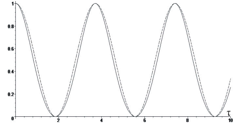
Figure 2: Comparison of the functions $\mbox{cn}^{2}\left(\tau,\frac{1}{\sqrt{2}}\right)$ and $\frac{1}{2}[1+\cos(\Omega\tau)]$.

Introducing a new time variable according to the formula $\Omega\tau=2\tilde{t}+\pi$, we obtain from Eq. (44):

$$\ddot{\tilde{z}}+\frac{2\Lambda}{\Omega^{2}}[1-\cos(2\tilde{t})]\cdot\tilde{z}(\tilde{t})=0.$$ (46)

Obviously, this is the Mathieu equation (42) with

$$a=\frac{2\Lambda}{\Omega^{2}}\;\;\;{\mbox{and}}\;\;\;q=\frac{\Lambda}{\Omega^{2}}.$$ (47)

Thus, we obtain a certain relation between two arbitrary parameters of Eq. (42):

$$a=2\,q.$$ (48)

Let us now recall the well-known stability diagram for the Mathieu equation (see, for example, l16 ). In Fig. 3, the regions of unstable motion are shaded.

The boundary lines $a_{i}(q)$, $b_{i}(q)$ ($i=1,2$) of these regions can be approximated by the following series:

$b_{1}(q)=1-q-\dfrac{q^{2}}{8}+\dfrac{q^{3}}{64}-\dfrac{q^{4}}{1536}+...$,

$a_{1}(q)=1+q-\dfrac{q^{2}}{8}-\dfrac{q^{3}}{64}-\dfrac{q^{4}}{1536}+...$,

$b_{2}(q)=4-\dfrac{q^{2}}{12}+\dfrac{5q^{4}}{13824}+...$,

$a_{2}(q)=4+\dfrac{5q^{2}}{12}-\dfrac{763q^{4}}{13824}+...$.

In Fig. 3, we also depict the straight line $a=2q$ according to Eq. (48) and four points ($A$,$B$,$C$,$D$) of the intersection of this line with the boundary curves $b_{i}(q)$, $a_{i}(q)$ ($i=1,2$). The following values of $q$ correspond to these points of intersection:

$q_{A}=0.329$, $\;\;q_{B}=0.890$, $\;\;q_{C}=1.858$, $\;\;q_{D}=2.321.$

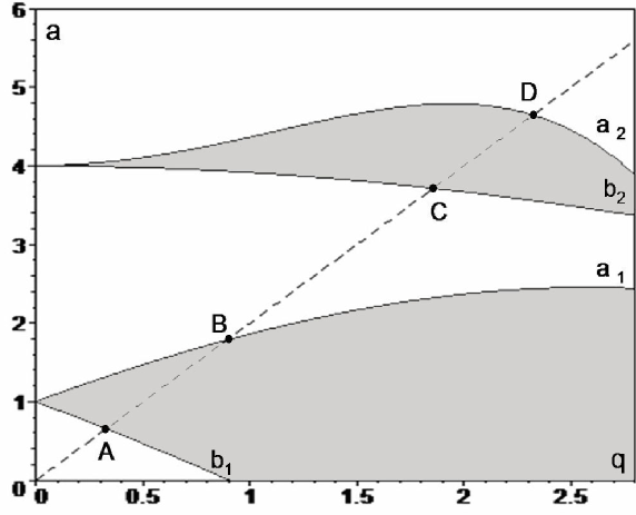
Figure 3: The regions of stable and unstable motion for the Mathieu equation.

On the other hand, $q=\frac{\Lambda}{\Omega^{2}}$ (see Eq. (47)) and, therefore, we can approximately find the values of the parameter $\Lambda$ corresponding to the boundaries of stable and unstable motion for the basic equation (44). In this way, we obtain the regions represented in the first column of Table 7.

Thus, there exist regions of stable and unstable motion for our basic equation (44) in accordance with the numeric values of the parameter $\Lambda$ entering this equation.

The above approach based on the Mathieu equation analysis not only sheds light on the main properties of Eq. (44), but allows us to arrive at some approximate results presented in Table 7. On the other hand, we can obtain analogous results with high precision analyzing the basic equation (44) with the aid of the Floquet method.

To this end, we construct the $2\times 2$ monodromy matrix by integrating Eq. (44) twice (with the initial conditions $z(0)=1$, $z^{\prime}(0)=0$ and $z(0)=0$, $z^{\prime}(0)=1$) over one period of the function $\mbox{cn}\left(\tau,\frac{1}{\sqrt{2}}\right)$ and calculate its multiplicators. If the absolute value of a multiplicator exceeds unity by more then $10^{-5}$, we identify the case of unstable motion.

The results obtained by the Floquet method prove to be surprising! Indeed, all boundary values of $\Lambda$ are integer numbers, at least up to $10^{-5}$:

$\Lambda_{A}=1$, $\;\;\Lambda_{B}=3$, $\;\;\Lambda_{C}=6$, $\;\;\Lambda_{D}=10$.

We suspect that this property of Eq. (44) can be proved exactly, but we could not find a proof of this conjecture .

Thus, for Eq. (44), we obtain the regions of stable and unstable motion presented in the second column of Table 7.

Table 7: Regions of stable and unstable motion for Eq. (44)

Analysis based on the Mathieu equation	Exact Floquet analysis	Stable or unstable motion
$0<\Lambda<0.945$	$0<\Lambda<1$	stable
$0.945<\Lambda<2.554$	$1<\Lambda<3$	unstable
$2.554<\Lambda<5.335$	$3<\Lambda<6$	stable
$5.335<\Lambda<6.665$	$6<\Lambda<10$	unstable

IV.3 Quasibreathers in the $K_{4}$-chains

The above results for the basic equation (44) allow us to make a final step in our breather stability analysis. Indeed, we have reduced this analysis to the problem of stability of the zero solutions to $\tilde{N}$ individual equations (43). A given breather will be stable, if all the values $\Lambda_{j}=\dfrac{3\lambda_{j}}{p^{2}}\;\;\;(j=-N..N)$ from Eq. (43) fall into certain regions of stability motion of the basic equation (44).

With high precision, we have computed the eigenvalues $\lambda_{j}$ of the matrix $A$ [see, for example, Eqs. (35-37)] and the values $\Lambda_{j}=\dfrac{3\lambda_{j}}{p^{2}}$ entering the basic equation (44) for the $K_{4}$-chain with different number of particles ($\tilde{N}$) and different values of the parameter $\beta$ determining the strength of the intersite potential. It has been revealed that all $\Lambda_{j}$, with exception of $\Lambda_{1}$, depend considerably on $\beta$ and slightly on $\tilde{N}$.

On the other hand, $\Lambda_{1}=3$ for all $\tilde{N}$ and $\beta$ and this constant coincides, at least up to $10^{-10}$, with the boundary between the first region of unstable and the second region of stable motion of the basic equation (44) [see Table 7]. Because of the importance of the equality $\Lambda_{1}=3$, we prove it analytically for $\tilde{N}=3$ in Appendix 1.

According to the Floquet theory, this means that a strictly time-periodic solution corresponds to $\Lambda_{1}=3$. Moreover, the eigenvector $\bm{V}_{1}$ of the matrix $A$, corresponding to $\Lambda_{1}$, remarkably coincides with high precision (see also Appendix 1 for the analytical proof of this fact for the case $\tilde{N}=3$) with the spatial profile of the considered breather for all $\tilde{N}$ and $\beta$. Therefore, the infinitesimal perturbation along the vector $\bm{V}_{1}$ does not relate to the stability of the breather: it leads only to the infinitesimal increasing of the breather’s amplitude. Thus, studying the breather stability, we must consider only $\Lambda_{j}$ with $j\neq 1$.

In Table 8, for $\beta=0.3$, we present the eigenvalues $\lambda_{j}$ of the matrix $A$ and the corresponding values $\Lambda_{j}$ for the $K_{4}$-chains with $\tilde{N}=3,5,7,9$ particles. It may be concluded, from this table, that for $\tilde{N}\geq 7$ only $\Lambda_{2}$, $\Lambda_{3}$, $\Lambda_{4}$ and $\Lambda_{5}$ are of considerable magnitude and correct values of these $\Lambda_{j}$, at least up to $10^{-5}$, can be found already from the case $\tilde{N}=5$. From Table 7, we also see that all $\Lambda_{j}$  ($j>1$) fall into the first region of stability ($0<\Lambda_{j}<1$) and, therefore, the considered breathers are stable for $\beta=0.3$.

Table 8: Eigenvalues of the matrix A of the linearized dynamical system for the $K_{4}$-chain with different number of particles $\tilde{N}$ ($\beta=0.3$)

$\tilde{N}=3$		$\tilde{N}=5$
$\lambda_{1}=2.298373452$	$\Lambda_{1}=3$	$\lambda_{1}=2.316036234$	$\Lambda_{1}=3$
$\lambda_{2}=0.5880160166$	$\Lambda_{2}=0.7675201995$	$\lambda_{2}=0.6248090298$	$\Lambda_{2}=0.8093254611$
$\lambda_{3}=0.2934494449$	$\Lambda_{3}=0.3830310231$	$\lambda_{3}=0.3226215801$	$\Lambda_{3}=0.4178970630$
		$\lambda_{4}=0.02626701223$	$\Lambda_{4}=0.03402409500$
		$\lambda_{5}=0.02530830363$	$\Lambda_{5}=0.03278226390$
$\tilde{N}=7$		$\tilde{N}=9$
$\lambda_{1}=2.316036234$	$\Lambda_{1}=3$	$\lambda_{1}=2.316036234$	$\Lambda_{1}=3$
$\lambda_{2}=0.6248090398$	$\Lambda_{2}=0.8093254740$	$\lambda_{2}=0.6248090398$	$\Lambda_{2}=0.8093254740$
$\lambda_{3}=0.3226216094$	$\Lambda_{3}=0.4178971017$	$\lambda_{3}=0.3226216094$	$\Lambda_{3}=0.4178971017$
$\lambda_{4}=0.02627089232$	$\Lambda_{4}=0.03402912093$	$\lambda_{4}=0.02627089232$	$\Lambda_{4}=0.03402912093$
$\lambda_{5}=0.02531216336$	$\Lambda_{5}=0.03278726346$	$\lambda_{5}=0.02531216336$	$\Lambda_{5}=0.03278726346$
$\lambda_{6}=0.3886030305e-5$	$\Lambda_{6}=0.5033639268e-5$	$\lambda_{6}=0.3886030305e-5$	$\Lambda_{6}=0.5033639268e-5$
$\lambda_{7}=0.3886011392e-5$	$\Lambda_{7}=0.5033614770e-5$	$\lambda_{7}=0.3886011392e-5$	$\Lambda_{7}=0.5033614770e-5$
		$\lambda_{8}=0.1094511318e-16$	$\Lambda_{8}=0.1417738596e-16$
		$\lambda_{9}=0.1094511318e-16$	$\Lambda_{9}=0.1417738596e-16$

In Fig. 4, we present the solution to Eq. (44) for $\Lambda_{2}$, $\Lambda_{3}$, $\Lambda_{4}$, $\Lambda_{5}$ corresponding to a certain initial amplitude (the value of this amplitude is inessential because Eq. (44) is linear). They are not periodic, but stationary solutions in the sense that their amplitudes don’t increase infinitely in time, as it occurs for the case where $\Lambda_{j}$ fall into an unstable region. Thus, if we are in a close (even infinitesimal) vicinity of a given breather, i.e. if all $\tilde{\delta}_{j}(t)$ [see Eq. (41)] are small values at the initial instant $t=0$, they continue to be small for all later times $t>0$. Then according to Eq. (38), the smallness of the Chebyshev norm $\|\tilde{\delta}_{j}(t)\|_{c}$ implies the smallness of $\|\delta_{j}(t)\|_{c}$.

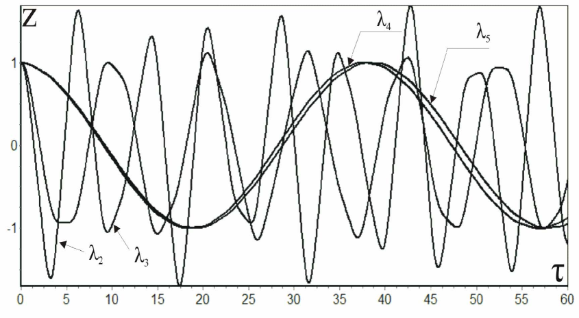
Figure 4: Solutions to the basic equation (44) corresponding to different values of $\Lambda$.

On the other hand, it follows from Eq. (38) that the solution to the original nonlinear equation (9) is not periodic in any small vicinity of the exact breather! Indeed, because of the relation $\bm{\delta}(t)=S\tilde{\bm{\delta}}(t)$, each $\delta_{j}(t)$ is a certain linear combination of all the $\tilde{\delta}_{j}(t)\;\;\;(j=-N..N)$, but individual $\tilde{\delta}_{j}(t)$ are, in general, quasiperiodic functions. [Even if certain $\tilde{\delta}_{j}(t)$ would be periodic, their periods are independent of each other and, therefore, the total solution $\delta_{j}(t)\;\;\;(j=-N..N)$ will not be periodic in any case.]. In other words, we arrive at the conclusion that arbitrary small vicinity of the exact breather solution consist of quasiperiodic solutions which can be naturally called quasibreathers.

Moreover, in the case of the $K_{4}$-chains with $\beta=0.3$, these quasibreathers turn out to be stable dynamical objects. Indeed, in a sufficiently small vicinity of the exact breather, the quasibreathers are described by the vector $\bm{x}(t)=\bm{x}_{b}(t)+\bm{\delta}(t)$ [see Eqs. (33) and (34)] where dynamics of $\bm{\delta}(t)$ is determined by the linearized system (35). Above we have demonstrated that all $\parallel\delta_{j}(t)\parallel_{c}$ are certainly small for any $t>0$. Therefore, one can conclude that not only the considered breather solution, but also the quasibreather solutions, which are close to it, must be stable in the Chebyshev norm.

Actually, in the $K_{4}$-space, there exist a certain one-dimensional family of the exact breathers with different amplitudes $A_{0}=x_{0}(0)$ and with the same spatial profile (see, Tables 3, 4, 5, 6). A straight line corresponds to this family in the $\tilde{N}$-dimensional space of all the conceivable initial conditions $x_{i}(0)\;\;\;(i=-N..N).$ It is practically impossible to tune exactly onto this specific line in the many-dimensional space.

On the other hand, in any vicinity of this line, we have to deal with the quasibreathers: the different particles possess different frequencies and, moreover, these frequencies evolve in time. Such a behavior of the individual particles in a quasibreather vibration in the $K_{4}$-chain can be illustrated by the method used in Sec. 2 for studying the James breathers.

We investigate the stability of the quasibreather solutions by direct numerical integration of the differential equations (9) of the considered chain over large time intervals. To this end, we choose a certain initial deviation

$$\bm{\delta}(0)=\varepsilon\cdot\{\delta_{-N}(0),...,\delta_{0}(0),...,\delta_{N}(0)\}$$ (49)

from the exact spatial profile $\bm{x}_{b}(0)$ of a given breather, where $\varepsilon$ is a small parameter, while $\delta_{n}(0)$  [$n=-N..N$] are random numbers whose absolute values don’t exceed unity. Then we solve Eq. (9) with initial condition $\bm{x}(0)=\bm{x}_{b}(0)+\bm{\delta}(0)$,  $\dot{\bm{x}}(0)=0$ and examine the numerical solution $\bm{x}(t)=\{x_{-N}(t),...,x_{0}(t),...,x_{N}(t)\}$ after a long time. We can scan any vicinity of the exact breather by varying $\varepsilon$ and the random sequence $\{\delta_{n}(0)\ |\ n=-N..N\}$ from Eq. 49. In Table 9, we present the results of such a calculation for the $K_{4}$-chain with $\tilde{N}=7$ and $\beta=0.3$. We have used the fourth-order Runge-Kutta method with time step $h=0.001$ and integrated Eq. (9) up to $t=1500T_{0}$, where $T_{0}$ is the period of the $\pi$-mode ($T_{0}=\pi$). The frequencies ($\omega_{j}$) of only five breather particles ($j=-2..2$) have been taken into account, because the vibrational amplitudes of the particles with $j=\pm 3$ are very small (they are of the order of $10^{-8}$).

Table 9: Derviations in frequencies of different breather (quasibreather) particles

	$\varepsilon=0$	$\varepsilon=10^{-7}$	$\varepsilon=10^{-6}$	$\varepsilon=10^{-5}$	$\varepsilon=10^{-4}$	$\varepsilon=10^{-3}$
$\omega_{-2}$	1.289333684	1.289324677	1.289226737	1.288414794	1.252673857
$\omega_{-1}$	1.289333684	1.289333939	1.28933311	1.289297098	1.289077907	1.287039954
$\omega_{0}$	1.289333684	1.28933432	1.289333134	1.289332824	1.2893981453	1.2933772905
$\omega_{1}$	1.289333684	1.289333847	1.289332133	1.289281901	1.2890993617	1.2887949577
$\omega_{2}$	1.289333684	1.289320432	1.289203072	1.288248186	1.2767350998
$\eta$	0	2.8923591607e-6	2.911839882e-5	2.397956354e-4	7.103135734e-3	1.8891448851e-3
$\eta_{max}$	1.261367077e-10	1.0051826702e-6	1.0272244997e-5	1.002013005e-4	1.000467033e-2	2.443460953e-1

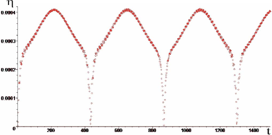
Figure 5: Mean square deviations $\eta=\eta(t_{k})$ in frequencies of the breather (quasibreather) particles for $\varepsilon\approx 10^{-9}$. Time $t$ is given in periods $T_{0}$.

Figure 6: Mean square deviations $\eta=\eta(t_{k})$ in frequencies of the breather (quasibreather) particles for $\varepsilon\approx 10^{-6}$. Time $t$ is given in periods $T_{0}$.

In Table 9, we also present the mean square deviations $\eta=\eta(t_{k})$ for $\omega_{j}$ determined by Eq. (6), which have been computed for $t_{k}\approx 1500T_{0}$, and the maximal values of $\eta(t_{k})$ for the interval $0<t_{k}<1500T_{0}$. The fact is that $\eta(t_{k})$ varies on the considered time interval (see, for example, Figs. 5, 6) and, therefore, $\eta_{max}$ is a more relevant characteristics of the deviations in frequencies of the individual particles.

From Table 9, one can see the specific quasibreather phenomenon, namely, the deviations in the frequencies $\omega_{j}$ of the individual particles increases with increasing the parameter $\varepsilon$, characterizing the deviation of the quasibreather shape from that of the exact breather in the Chebishev norm. It is important to emphasize that despite different particles possess slightly different frequencies $\omega_{j}$, the quasibreathers are stable dynamical objects. Indeed, we did not observe any decay of these objects for $\varepsilon\leq 10^{-2}$ up to $t=10^{6}T_{0}$ ($\eta_{max}$, even for such time interval, does not practically differ from those presented in Table 9).

However, for $\varepsilon>10^{-2}$, we have observed the decay of the quasibreathers which manifest itself in appearance of appreciable vibrational amplitudes of those particles whose amplitudes were practically equal to zero in the exact breather solution.

In conclusion, let us return to Figs. 5 and  6, where we depict $\eta(t_{k})$ as a function of the subsequent instants $t_{k}$ for which the frequencies $\omega_{j}$ were calculated. Sometimes, the function $\eta(t_{k})$ demonstrate regular oscillations, sometimes, practically chaotic oscillations. Such a behavior can be understood, if one takes into account that the displacement of each particle is a superposition of different quasiperiodic functions, as it was shown above in the present section.

IV.4 Stability of breathers with respect to strength of intersite potential

We consider the $K_{4}$-chain determined by the potential energy (8) inducing the Newton dynamical equations ($\ddot{x}_{n}=-\dfrac{\partial U}{\partial{x_{n}}}$) in the form (9). Let us discuss the stability of the breathers and quasibreathers in this chain with respect to the parameter $\beta$ which determines the strength of the intersite part of the potential energy relative to its on-site part. Eigenvalues $\lambda_{j}$ of the matrix $A$ from Eq. (35) and, therefore, the corresponding values $\Lambda_{j}$ of the parameter $\Lambda$ entering Eq. (44), depend on $\beta$: $\lambda_{j}=\lambda_{j}(\beta)$, $\Lambda_{j}=\Lambda_{j}(\beta)$.

In Fig. 7, we present $\Lambda_{j}(\beta)$ with $j=2,3,4,5$ for the $K_{4}$-chain with $\tilde{N}=3,\,5,\,7,\,9$ particles. These $\Lambda_{j}(\beta)$ are of the more significant values, as it follows from Table 8. All $\Lambda_{j}(\beta)$ which are not depicted in Fig. 7 are small positive numbers. Then one can conclude that for $\beta\in[0,0.554]$ all $\Lambda_{j}(\beta)$ remain in the first stability region ($0<\Lambda<1$) of the basic equation (44). As it has been already discussed this demonstrates the stability of the considered breathers (and, therefore, quasibreathers which are close to them) when $\beta$ increases from zero up to $\beta_{c}=0.554$. (Note that our breathers are unstable for $\beta<0$).

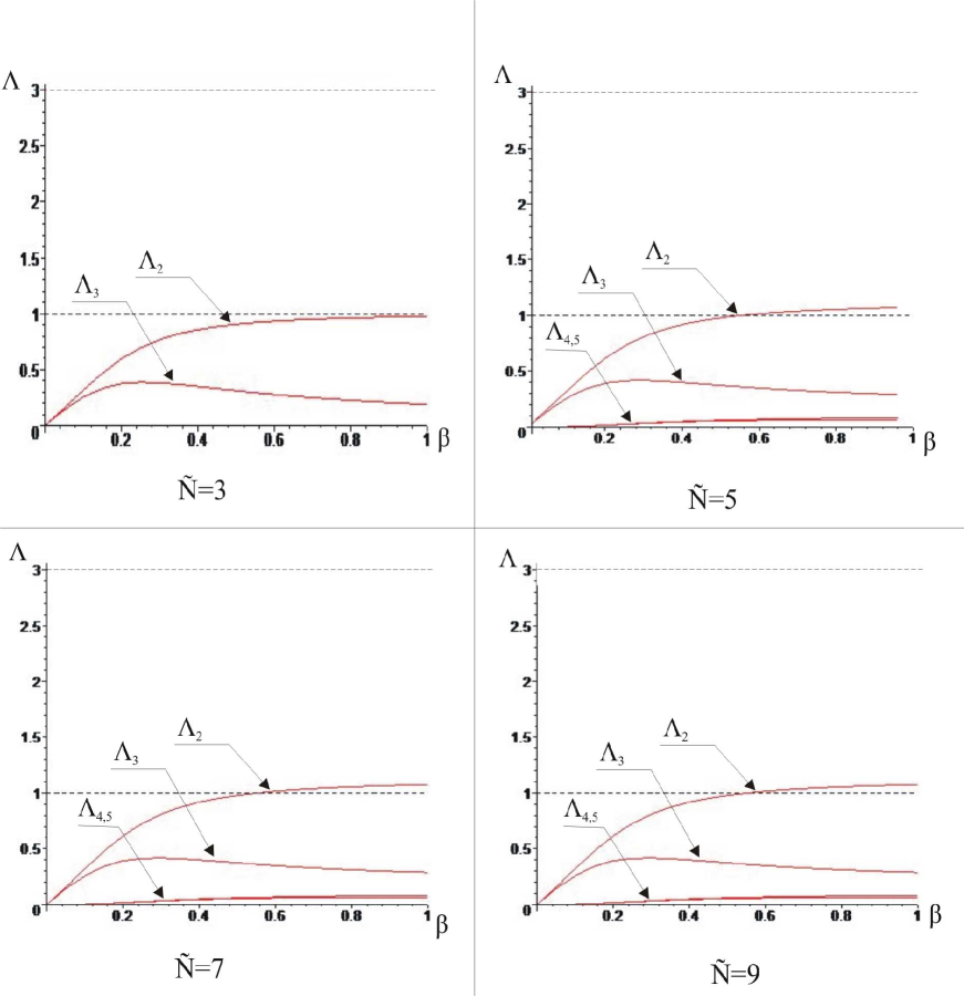
Figure 7: The functions $\Lambda_{j}(\beta)$ for different eigenvalues of the matrix A for the $K_{4}$-chain with $\tilde{N}=3,\,5,\,7,\,9$ particles. Note that the plots of $\Lambda_{4}(\beta)$ and $\Lambda_{5}(\beta)$ practically coincide with each other (see Table 8 for $\tilde{N}=9$).

On the other hand, we find from Fig. 7 that $\Lambda_{2}$ intersects the upper boundary ($\Lambda=1$) of the first stability region for $\tilde{N}>3$ when $\beta$ exceeds $0.554$. This implies the loss of stability of the breathers in the considered $K_{4}$-chain.

Thus, the intersite part of the potential with $\beta>0$ must not be too large with respect to its on-site part ($\beta<0.554$) for breathers (quasibreathers) to be stable.

Finally, let us point out an one-dimensional subspace of the space of all possible displacements which becomes unstable when $\beta$ intersects the critical value $\beta_{c}=0.554$. This subspace is determined by the eigenvector $\bm{V}$ corresponding to $\lambda_{2}$:

$\bm{V}=[0.05266431305,-0.7051428715,0,0.7051428725,-0.05266431306].$

V Conclusion

The main conclusion of the present paper is that the conventional view on the discrete breathers as strictly time periodic and spatially localized dynamical objects must be revised in a certain sense. Indeed, it has been shown here that for the James breathers l4 ; l5 in the $K_{2}-K_{3}-K_{4}$ chain as well as for the breathers in the $K_{4}$-chain with on-site and intersite potentials we actually deal with the dynamical objects representing quasibreathers: there are certain deviations in the vibrational frequencies of the individual particles. These deviations can be characterized by the mean square deviation which certainly exceeds the possible numerical errors. Moreover, for the case of the $K_{4}$-chain, we have performed a rigorous investigation of the existence and stability of such quasibreathers. For the $K_{4}$-chain, the exact breathers exist only along a certain line in the many-dimensional space of all the possible initial conditions, and it is actually impossible to tune precisely onto this line in any physical and computational experiments.

In some of our numerical experiments with the $K_{4}$-chain, the deviations in frequencies of the vibrating particles from the average quasibreather frequency $\omega_{b}$ attained 1%, but possibly these deviations can considerably exceed this value for more realistic models.

The deviations in frequencies of the individual particles (and in frequency of the given particle over time) result in some change of the breather Fourier spectrum, namely, instead of the ideal lines at the breather frequency $\omega_{b}$ and its multiples there appear certain (possibly, narrow) packets of the Fourier components near the ideal breather lines and near zero frequency. This effect is difficult to reveal with the aid of the numerical Fourier analysis and we prefer to study the deviations in vibrational frequencies of the individual particles in the straightforward way.

It is essential, that the above described deviations in frequencies of the individual vibrating particles, in general, don’t mean an onset of the breather decay. We have demonstrated this fact with the example of stable quasibreathers in the $K_{4}$-chain. For this case, we succeeded in proving that these quasibreathers turn out to be stable up to a certain strength of the intersite potential with respect to the on-site potential.

We conjecture that the results obtained in the present paper for two particular cases (the James breathers and the breathers in the $K_{4}$-chain) are also valid for the general case and, therefore, one must speak about quasibreathers rather than about strictly time-periodic breathers.

Finally, let us note that the term ”quasiperiodic breathers” is used in literature for dynamical objects different from the quasibreathers considered in the present paper (for example, see l17 and the references therein). Indeed, the former possess several basis frequencies (and their integer linear combinations) in the Fourier expansion with substantial amplitudes, while the latter possess only one basis frequency $\omega_{b}$ (and its multiples), as well as many small components with frequencies different from $n\omega_{b}$. The quasiperiodic breathers exist only in rather specific cases, while quasibreathers seam to be the generic dynamical objects.

Appendix A

In Sec. IV.3, using straightforward numerical calculations, we have demonstrated that the largest eigenvalue $\lambda_{1}$ of the matrix $A$ [see Eqs. (35-37)] corresponds to the boundary between the first unstable and the second stable regions for the basic equation (44). Moreover, the eigenvector $\bm{V_{1}}$, associated with $\lambda_{1}$, determines the direction of the infinitesimal perturbation along the considered breather.

Below we prove these propositions analytically for the $K_{4}$-chain with $\tilde{N}=3$ particles. Let us consider Eq. (35)

$$\ddot{\bm{\delta}}=-3x_{0}^{2}(t)\cdot A\bm{\delta}$$ (50)

with matrix $A$ determined by Eq. (36). The parameter $k$ entering the matrix $A$ determines the spatial profile

$$\{k,1,k\}$$ (51)

of the breather

$$\{kx_{0}(t),x_{0}(t),kx_{0}(t)\},$$ (52)

while time dependence of the breather particles can be obtained from equations (24,25):

$$\ddot{x}_{0}+p^{2}x_{0}^{3}=0,$$ (53)

$$p^{2}=1+2\beta(1-k)^{3}.$$ (54)

On the other hand, parameter $k=k(\beta)$ is a function of the intersite potential stregth $\beta$, as it follows from Eqs. (19):

$$k(1+k)+\beta(1-k)^{2}(1+2k)=0.$$ (55)

The eigenvalues $\lambda_{j}$ ($j=1,2,3$) of the matrix $A$ can be calculated from the characteristic equation of this matrix in the following form:

$$\lambda_{1,3}(\beta)=\frac{1}{2}[(1+k^{2})+3\beta(1-k)^{2}]\pm\frac{1}{2}(1-k)\sqrt{(1+k)^{2}+2\beta(1-k^{2})+9\beta^{2}(1-k)^{2}},$$ (56)

$$\lambda_{2}(\beta)=k^{2}+\beta(k-1)^{2}.$$ (57)

In principle, one can obtain these eigenvalues as explicit functions of the intersite potential strength $\beta$ from Eq. (55) and substitute it into Eqs. (56) and (57). This way is too cumbersome and we prefer to use the following trick. Let us express $\beta$ via $k$ from Eq. (55) and substitute $\beta=\beta(k)$ into Eqs. (56, 57). Then, the square root entering Eq. (56) can be explicitly extracted and written in the form

$$\frac{(1+k)(1+2k^{2})}{1+2k}.$$ (58)

As a consequence of this extraction, we obtain

$$\lambda_{1}=\frac{1+2k^{3}}{1+2k},$$ (59)

$$\lambda_{3}=-k.$$ (60)

The same substitution of $\beta=\beta(k)$ into Eqs.(57) and (54) permits us to write $\lambda_{2}$ and $p^{2}$ as follows:

$$\lambda_{2}=\frac{k(1-2k^{2})}{1+2k},$$ (61)

$$p^{2}=\frac{1+2k^{3}}{1+2k},$$ (62)

Comparing Eqs. (59) and (62), we obtain

$$\lambda_{1}(\beta)=p^{2}(\beta).$$ (63)

This is an important result since our basic equation (44) reads

$$z^{\prime\prime}+\Lambda x_{0}^{2}(\tau)x(\tau)=0,$$ (64)

with

$$\Lambda=\dfrac{3\lambda}{p^{2}(\beta)}.$$ (65)

Then, we can conclude that $\Lambda_{1}=\dfrac{3\lambda_{1}}{p^{2}(\beta)}=3$ and, therefore, $\Lambda_{1}$ is a constant with respect to the intersite potential strength $\beta$! Moreover, as already has been discussed in Sec IV.3, this value turns out to be the exact boundary between the first region of unstable motion ($1<\Lambda<3$) and the second region of stable motion ($3\leq\Lambda\leq 6$) of the basic equation (64).

Let us recall that numerical calculations have convinced us with high precision that $\Lambda_{1}=3$ not only for the case $\tilde{N}=3$, but for any other number of the particles in the $K_{4}$-chain. Moreover, it can be proved that $\Lambda_{1}=m$ for the uniform potential of the arbitrary order $m$ (in the present paper, we consider only the case $m=3$).

The eigenvectors $\bm{V}_{j}$ ($j=1,2,3$) of the matrix $A$ corresponding to $\lambda_{j}$ from Eqs. (59-61) can be written after the substitution $\beta$ from Eq. (55) as follows:

$$\bm{V}_{1}=[k,1,k],\bm{V}_{2}=[-1,0,1],\bm{V}_{3}=[1,-2k,1],$$ (66)

where $k=k(\beta)$. We see that $V_{1}=[k,1,k]$ represents the vector which coincides exactly with the spacial profile (51) of the considered breather. On the other hand, $\bm{V}_{j}$ ($j=1,2,3$) are the eigenvectors of the matrix $A$ [see Eq. (50)] of the dynamical equations of the $K_{4}$-chain linearized near the breather (52). Therefore, $\bm{V}_{1}=[k,1,k]$, corresponding to $\Lambda=3$, determines the direction along our breather in the three-dimensional space of all the displacements of the particles. In Section IV, using numeric calculations with high precision, we have already arrived at the conclusion that this result turns out to be correct not only for the case $\tilde{N}=3$, but also for the $K_{4}$-chain with arbitrary number of particles.

References

- (1) S. Aubry, Physica D 103, 201 (1997).
- (2) S. Flach and C. R. Willis, Phys. Rep. 295, 181 (1998).
- (3) S. Flach, Computational studies of discrete breathers, in ”Energy Localization and Transfer”, Eds. T. Dauxois, A. Litvak-Hinenzon, R. MacKay and A. Spanoudaki, World Scientific, pp.1-71 (2004).
- (4) G. James, C.R. Acad.Sci.Paris, t. 332, Ser.1, p.581 (2001); G. James, J. Nonlinear Sci. 13, 27 (2003).
- (5) B. Sanchez-Rey, G. James, J. Cuevas and J.F.R. Archilla. Phys. Rev. B 70, 014301 (2004).
- (6) R. M. Rosenberg, J. Appl. Mech. 29, 7 (1962).
- (7) R. M. Rosenberg, Adv. Appl. Mech. 9, 155 (1966).
- (8) Yu. S. Kivshar, Phys. Rev. E 48, R43 (1993).
- (9) S. Flach, Phys. Rev. E 51, 1503 (1995).
- (10) G.M. Chechin, N.V. Novikova, and A.A. Abramenko, Physica D 166, 208 (2002).
- (11) G.M. Chechin, D.S.Ryabov, and K.G.Zhukov, Physica D 203, 121 (2005).
- (12) V.P. Sakhnenko and G.M. Chechin, Dokl. Akad. Nauk 330, 308 (1993); 338, 42 (1994) [Phys. Dokl. 38, 219 (1993); 39, 625 (1994)];
- (13) G.M. Chechin and V.P. Sakhnenko, Physica D 117, 43 (1998).
- (14) G.M. Chechin, V.P. Sakhnenko, H.T. Stokes, A.D. Smith, and D.M. Hatch, Int. J. Non-Linear Mech. 35, 497 (2000).
- (15) G.M. Chechin, A.V. Gnezdilov, and M.Yu. Zekhtser, Int. J. Non-Linear Mech. 38, 1451 (2003).
- (16) M. Abramowitz and I.A. Stegun, Eds., Handbook of Mathematical Functions (Dover Publications, Inc., New York, 1965).
- (17) D. Bambusi and D.Vella. DCDS-B, 2, 389 (2002).