Periodic-Orbit Approach to

Universality in Quantum Chaos

Dissertation
zur Erlangung des Grades
Doktor der Naturwissenschaften
(Dr. rer. nat.)
vorgelegt am Fachbereich Physik der
Universität Duisburg-Essen
von
Sebastian Müller
aus Essen eingereicht: Essen, September 2005

Referent:	Prof. Dr. Fritz Haake
Korreferent:	Prof. Dr. Robert Graham

Abstract

We show that in the semiclassical limit, classically chaotic systems have universal spectral statistics. Concentrating on short-time statistics, we identify the pairs of classical periodic orbits determining the small-$\tau$ behavior of the spectral form factor $K(\tau)$ of fully chaotic systems. The two orbits within each pair differ only by their connections inside close self-encounters in phase space. The frequency of occurrence of these self-encounters is determined by ergodicity. Permutation theory is used to systematically sum over all topologically different families of such orbit pairs. The resulting expansions of the form factor in powers of $\tau$ coincide with the predictions of random-matrix theory, both for systems with and without time-reversal invariance, and to all orders in $\tau$. Our results are closely related to the zero-dimensional nonlinear $\sigma$ model of quantum field theory. The relevant families of orbit pairs are in one-to-one correspondence to Feynman diagrams appearing in the perturbative treatment of the $\sigma$ model.

Kurzfassung

Wir zeigen, dass klassisch chaotische Systeme sich im semiklassischen Limes durch die universelle Statistik ihrer Quantenspektren auszeichnen. Dabei konzentrieren wir uns auf das Kurzzeitverhalten des spektralen Formfaktors $K(\tau)$. Wir weisen nach, dass für dieses Verhalten Paare periodischer Bahnen verantwortlich sind, die sich voneinander nur durch ihre Verbindungen innerhalb naher Selbstbegegnungen im Phasenraum unterscheiden. Die Häufigkeit solcher Selbstbegegnungen wird durch die Ergodizität der klassischen Dynamik bestimmt. Wir verwenden Methoden der Permutationstheorie, um über alle topologisch verschiedenen Familien solcher Bahnpaare zu summieren. Die resultierenden Entwicklungen des Formfaktors in Potenzen von $\tau$ stimmen in allen Ordnungen mit den Vorhersagen der Zufallsmatrixtheorie überein, sowohl für zeitumkehrinvariante Systeme als auch für Systeme ohne Zeitumkehrinvarianz. Unsere Ergebnisse haben einen engen Bezug zum nulldimensionalen nichtlinearen $\sigma$-Modell der Quantenfeldtheorie. Die betrachteten Familien von Bahnpaaren entsprechen Feynman-Diagrammen, die bei der perturbativen Behandlung des $\sigma$-Modells auftreten.

Acknowledgement

I am extremely grateful to my thesis advisor, Prof. Fritz Haake, for giving me the opportunity to work on this interesting topic, and for his continuous interest and support.

I also wish to thank Prof. Robert Graham for agreeing to co-referee this thesis.

Most of this thesis is part of a very close and enjoyable cooperation with Prof. Petr Braun, Prof. Fritz Haake, and Stefan Heusler. Later, Prof. Alexander Altland joined the team and provided crucial insights into field-theoretical aspects. It is a special pleasure to thank all of them for this great experience and for many important contributions. Furthermore, I am indebted to Petr Braun, Fritz Haake, and Stefan Heusler for their comments on the manuscript.

I also want to thank Marko Turek, Dominique Spehner, and Prof. Klaus Richter for the joint work on our publication [21], containing results on multi-dimensional systems included in this thesis.

I am grateful to my colleagues Sven Biermann, Julia Ernst, Thorsten Feldmann, Gregor Hackenbroich, Birgit Hein, Konstantin Krutitsky, Philipp Kuhn, Andrea Lambert, Christopher Manderfeld, Bernhard Mieck, Axel Pelster, Wieland Ronalter, Dima Savin, Holger Schaefers, Urs Schreiber, Lionel Sittler, Prof. Hans-Jürgen Sommers, Prof. Stefan Thomae, Matthias Timmer, and Carlos Viviescas for the pleasant working atmosphere and numerous interesting discussions.

During conferences, seminars, and visits, I enjoyed helpful discussions with Arnd Bäcker, Prof. Gregory Berkolaiko, Prof. Bruno Eckhardt, Sven Gnutzmann, Prof. Gerhard Knieper, Jan Müller, Jens Marklof, Prof. Jürgen Müller, Prof. Taro Nagao, Holger Schanz, Henning Schomerus, Martin Sieber, Prof. Ben Simons, Prof. Uzy Smilansky, Wen-ge Wang, and Prof. Martin Zirnbauer.

I am grateful to Barbara Sacha for help with organizational problems, and to Rüdiger Oberhage who maintained our computer system and was always available for questions.

This work was supported by the Sonderforschungsbereich TR/12 “Symmetries and Universality in Mesoscopic Systems” of the Deutsche Forschungsgemeinschaft.

Finally, I am grateful to my parents for all they have done for me.

Kapitel 0 Introduction

Chaotic quantum systems display universal behavior [1, 2]. Their energy eigenvalues have universal statistics, and show a tendency to repel each other. The conductance and shot noise of chaotic quantum dots are of universal form, as well as the fluctuations of cross sections in chaotic scattering systems. Many more examples for universality can be found in diverse ares ranging from quantum chromodynamics and molecular spectroscopy to the study of normal-metal/superconductor heterostructures.

A quantitative prediction of such universal features is possible if, rather than considering an individual system, we average over all Hamiltonians (represented by large matrices) sharing the same symmetry properties. This approach, termed random-matrix theory, was pioneered by Wigner and Dyson in the 1950s, for the level statistics of atomic nuclei [3, 4]. Surprisingly, the predictions of random matrix theory, even though derived using ensembles of matrices, are typically respected even by individual chaotic dynamics. Growing evidence for the success of random-matrix theory outside of its initial realm of nuclear physics (see [5] for preceding works) led Bohigas, Giannoni, and Schmit [6] to conjecture that the statistics of energy levels of individual classically chaotic systems is faithful to random-matrix theory.

One of the fundamental problems of quantum chaos is to find a first-principles proof for this conjecture. The reasons (and conditions) for universality should be related to the classical signatures of chaos [7] displayed by the same type of systems. The classical time-evolution of chaotic dynamics depends sensitively on the initial conditions, a property known as hyperbolicity. Typically, a small initial separation between two trajectories will grow exponentially in time. Only separations along certain “stable” phase-space directions rather shrink exponentially. Moreover, chaotic dynamics are ergodic: Long trajectories uniformly fill the energy shell.

How can we relate universality to these classical manifestations of chaos? To answer this question, several approaches have been suggested, such as parametric level dynamics [2] or field-theoretical methods [8, 9, 10, 11]. Following pioneering work in [12, 13, 14, 15], our starting point will be Gutzwiller’s trace formula[16]. In the semiclassical limit, the level density of a (bounded) chaotic quantum system can be written as a sum over its classical periodic orbits. By Fourier transforming Feynman’s path integral for the (trace of) the time-evolution operator, we express the level density as an integral over classical trajectories closed in configuration space, with an integrand ${\rm e}^{{{\rm i}}S/\hbar}$ involving the classical action $S$. A stationary-phase approximation brings about a sum over trajectories extremizing the action – which are nothing but classical periodic orbits solving the equations of motion. Each orbit $\gamma$ then comes with a phase factor $\rm{e}^{{{\rm i}}S_{\gamma}/\hbar}$.

As a prominent example for universality, we will consider the two-point correlator of the level density, and its Fourier transform, the so-called spectral form factor $K(\tau)$. The form factor is naturally expressed as a function of a time variable $\tau$, conjugate to the energy difference; this time is made dimensionless by referral to the Heisenberg time $T_{H}\propto\hbar^{1-f}$ ($f$ denoting the number of degrees of freedom), the time scale associated to the mean level spacing. The prediction of random-matrix theory depends only on whether the system in question is time-reversal invariant or not. In absence of time-reversal invariance, we have to average over Hermitian matrices (the Gaussian Unitary Ensemble, GUE) and obtain $K(\tau)=\tau$. Time-reversal invariant systems require an average over real symmetric matrices (the Gaussian Orthogonal Ensemble, GOE), yielding $K(\tau)=2\tau-\tau\ln(1+2\tau)=2\tau-2\tau^{2}+2\tau^{3}-\ldots$. Here, we momentarily excluded complications due to spin or geometric symmetries and, most importantly, restricted ourselves to $\tau<1$. Broad experimental and numerical support suggests that individual chaotic systems are faithful to the above predictions if we (i) consider highly excited states (justifying the semiclassical limit $\hbar\to 0$), and (ii) perform two averages, usually over small intervals of energy and time, to turn $K(\tau)$ into a smooth and plottable function.

The form factor, involving a product of level densities, leads to a double sum over long periodic orbits $\gamma$, $\gamma^{\prime}$ with periods close to $\tau T_{H}$, and thus of the order of the Heisenberg time; the associated phase factor ${\rm e}^{{{\rm i}}(S_{\gamma}-S_{\gamma^{\prime}})/\hbar}$ depends on the difference between their classical actions. This double sum relates correlations in quantum spectra to correlations among the actions of classical orbits [13]. In the semiclassical limit, it may draw systematic contributions only from pairs of orbits with a small action difference, at most of the order of Planck’s constant. The contributions of all other orbit pairs will interfere destructively and effectively vanish after performing the two averages indicated above.

Following Berry [12], we first consider pairs of orbits with identical action. In absence of time-reversal invariance (or other degeneracies of the periodic-orbits spectrum), this leaves only pairs of identical orbits $\gamma=\gamma^{\prime}$. The resulting “diagonal” contribution $\tau$ coincides with the random-matrix result. In presence of time-reversal invariance, mutually time-reversed orbits must also be taken into account. The number of relevant orbit pairs is thus doubled. The overall contribution, $2\tau$, reproduces only the leading term of the GOE form factor.

Can this approach be extended to all orders of $K(\tau)$? As first seen numerically by Argaman et al. [13], off-diagonal orbit pairs are capable of producing additional contributions to the form factor. We know by now that one must account not only for pairs of orbits identical up to time reversal, but also for orbits composed of parts similar up to time reversal. Within each family of such orbit pairs, the action difference can be steered to zero, by varying parameters defining the family.

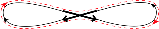
Abbildung 1: Sketch of a Sieber/Richter pair in configuration space: The partner orbits, depicted by solid and dashed lines, differ noticeably only inside an encounter of two orbit stretches (marked by opposite arrows, indicating the direction of motion). The sketch greatly exaggerates the difference between the two partner orbits in the loops outside the encounter and depicts the loops disproportionally short; similar remarks apply to all subsequent sketches of orbit pairs.

In a paradigmatic breakthrough, the first such family was identified by Sieber and Richter [14, 15], based on intuition drawn from quantum field theory [9, 10, 11]. Their original formulation is based on small-angle self-crossings in configuration space. Inside each Sieber/Richter pair ($\gamma$, $\gamma^{\prime}$), one orbit differs from its partner by narrowly avoiding one of its many self-crossings; see Fig. 1.

In phase-space language, both $\gamma$ and $\gamma^{\prime}$ contain a region (a so-called “encounter”) where two stretches of the same orbit are almost mutually time-reversed. Between the two encounter stretches, each orbit goes through two “loops”. The two orbits noticeably differ from each other only by their connections inside the encounter. In contrast, they practically coincide in one loop, and are mutually time-reversed in the other loop. The closer the stretches are, the smaller will be the resulting action difference $S_{\gamma}-S_{\gamma^{\prime}}$. Sieber/Richter pairs exist only for time-reversal invariant systems, where they give rise to the quadratic contribution to the form factor, $-2\tau^{2}$.

In this thesis, we will extend Sieber’s and Richter’s reasoning (first formulated for surfaces of constant negative curvature) to general chaotic dynamics and, moreover, extract all remaining terms in the power series of $K(\tau)$. To go beyond the quadratic approximation, we have to consider pairs of orbits differing in any number of encounters, with arbitrarily many stretches. For instance, the cubic contribution to the spectral form factor arises from pairs of orbits differing in either two close encounters each involving two stretches, or in one encounter of three stretches. See Fig. 2 for an example of an two partner orbits differing in one encounter of two and one encounter of three stretches, contributing to the order $\tau^{4}$.

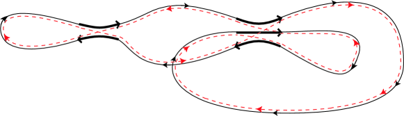
Abbildung 2: Periodic orbit $\gamma$ with one 2- and one 3-encounter highlighted, and a partner $\gamma^{\prime}$ obtained by reconnection.

We shall see how the classical signatures of chaos – hyperbolicity and ergodicity – determine the universal contributions of these orbit pairs to the spectral form factor. It is only due to hyperbolicity that we can obtain partner orbits via local reconnections inside encounters, leaving the intervening loops almost unaffected. Two different encounter stretches, respectively belonging to $\gamma$ and $\gamma^{\prime}$, may lead to approximately coinciding loops if their phase-space difference is close to the stable direction and thus shrinks exponentially in time. Hyperbolicity also determines the duration of an encounter. The stretches stay close as long as their exponential divergence permits. Hence, the duration of an encounter will be a logarithmic function of the smallest phase-space separations involved. Since the encounters relevant for spectral universality involve a separation of the order of a Planck cell, encounter durations will be of the order of Ehrenfest time $T_{E}\propto\ln\frac{\text{const.}}{\hbar}$ – divergent in the semiclassical limit, but much smaller than the orbit periods.

Furthermore, ergodicity determines the frequency of occurrence of close self-encounters inside long periodic orbits. We thus see that all system-specific properties fade away, leaving us indeed with universal contributions to the form factor. (The conditions mentioned here will be refined to guarantee that all classical time scales remain finite and thus negligible compared to $T_{H}$ and $T_{E}$.)

A second problem, decoupled from the phase-space considerations sketched above, is to systematically account for all families of orbit pairs differing in encounters. These families will be characterized not only by the number of related encounters and of the stretches involved, but also on the order in which stretches and loops are passed. To deal with this problem, we shall define the notion of “structures” of orbit pairs, and relate these structures to permutations. Roughly speaking, each structure corresponds to one way of reordering the loops $1,2,\ldots,L$ of $\gamma$ ($L$ denoting the total number of loops) to a new sequence in $\gamma^{\prime}$ – possibly changing the sense of traversal for dynamics with time-reversal invariance. Using the theory of permutations, we can determine by recursion the number of structures contributing to each order in $\tau$, and hence the Taylor coefficients of $K(\tau)$. The resulting series fully coincide with the predictions of random-matrix theory, both for systems with and without time-reversal invariance.

Our approach is closely related to the non-linear $\sigma$ model of quantum field theory. In its zero-dimensional version, that model provides an efficient way of implementing random-matrix averages of spectral correlators, or impurity averages for disordered rather than chaotic systems. An alternative approach to universality was even aimed at deriving a “ballistic” $\sigma$ model for individual chaotic systems, by investigating the underlying classical dynamics [8].

A perturbative implementation of the $\sigma$ model yields a diagrammatic expansion mirroring our expansion in terms of (families of) orbit pairs, with vertices corresponding to encounters and propagator lines corresponding to orbit loops. The present orbit pairs thus give a classical interpretation for Feynman diagrams. That said, it is no surprise that the importance of close self-encounters in periodic orbits was first realized in a field-theoretical context [9, 10, 11].

This thesis is organized as follows. To set up the stage we first want to review the necessary concepts from classical and quantum chaos.

We shall then move on to discuss the orbit pairs responsible for the two lowest orders of the spectral form factor. The treatment of Sieber/Richter pairs in Chapter 2 will exemplify the phase-space geometry of encounters. The separations between encounter stretches will be measured in a coordinate system spanned by the stable and unstable directions; Sieber’s and Richter’s original treatment in terms of crossing angles rather than phase-space coordinates, and our generalizations of this approach, will be the topic of a separate Appendix. The statistics of phase space-separation will be derived using (i) ergodicity and (ii) the necessity of having encounter stretches separated by non-vanishing loops. We shall see that indeed the leading off-diagonal contribution to the form factor, $-2\tau^{2}$, comes about.

In the fourth Chapter, we shall classify the orbit pairs responsible for the cubic contribution to $K(\tau)$, either involving two encounters of two, or one encounter of three orbit stretches. We will see that reconnections inside encounters may give rise to either one connected or several disjoint orbits; only connected partner orbits contribute to the form factor. We will summarize the lessons learned for more complicated orbit pairs, and precisely define the notion of “structures” of orbit pairs.

Thus prepared, we will attack the general problem in Chapters 4 and 5. In Chapter 4, we will investigate the phase-space geometry of encounters with arbitrarily many stretches. For each structure of orbit pairs, we will determine the corresponding density of phase-space separations. Integration leads to a simple formula for the contribution to the form factor arising from each structure.

Structures will be counted in Chapter 5 with the help of permutation theory, leading to a recursion for the Taylor coefficients of $K(\tau)$. In absence of time-reversal invariance, the contributions of all orbit pairs differing in encounters sum up to zero. For time-reversal invariant dynamics, we indeed recover the logarithmic behavior predicted by the GOE. This completes our semiclassical derivation of the random-matrix form factor.

In Chapter 6 we give a brief introduction to the bosonic replica variant of the nonlinear $\sigma$ model, and show that its perturbative implementation directly parallels our semiclassical treatment.

Conclusions will be presented in Chapter 7. We shall discuss open problems (such as the large-time behavior of $K(\tau)$), and point to interesting applications in mesoscopic physics.

Appendices will provide important details and extensions, e.g., an alternative treatment in terms of crossing angles, and generalizations to multidimensional and “inhomogeneously hyperbolic” systems. Moreover, we shall show that contributions to the form factor arise only from those encounters which have all their stretches separated by intervening loops.

Parts of the results of this thesis have been published in [17, 18, 19, 20, 21, 22].

Kapitel 1 Classical and quantum chaos

1 Classical chaos

In this thesis, we will be concerned with quantum properties of classically chaotic Hamiltonian systems. In particular, we need to introduce two notions of classical chaos: hyperbolicity and ergodicity; see [7] for a more detailed account.

1 Hyperbolicity

Roughly speaking, a system is hyperbolic if its time evolution depends sensitively on the initial conditions. To prepare for a more precise definition we introduce, for each phase-space point ${\bf x}=({\bf q},{\bf p})$, a Poincaré surface of section ${\cal P}$ orthogonal to the trajectory passing through ${\bf x}$. Assuming a Cartesian configuration space (and thus a Cartesian momentum space), ${\cal P}$ consists of all points ${\bf x}+\delta{\bf x}=({\bf q}+\delta{\bf q},{\bf p}+\delta{\bf p})$ in the same energy shell as ${\bf x}$ whose configuration-space displacement $\delta{\bf q}$ is orthogonal to ${\bf p}$. For systems with $f$ degrees of freedom, ${\cal P}$ is a $(2f-2)$-dimensional surface within the $2f-1$-dimensional energy shell. As long as two trajectories respectively passing through the points ${\bf x}$ and ${\bf x}+\delta{\bf x}$ in ${\cal P}$ remain sufficiently close, we may follow their separation by linearizing the equations of motion around one trajectory,

$$\delta{\bf x}(t)=M({\bf x}_{0},t)\delta{\bf x}(0).$$ (1)

Here $\delta{\bf x}(t)$ denotes the phase-space separation in a co-moving Poincaré section, transversal to ${\bf x}(t)$, the image of ${\bf x}(0)={\bf x}_{0}$ under time evolution over time $t$. The so-called stability matrix $M$ with $M_{ij}({\bf x}_{0},t)=\frac{\partial(\delta x_{i}(t))}{\partial(\delta x_{j}(0))}$ defines a linear map from the Poincaré section at ${\bf x}(0)$ to that at ${\bf x}(t)$.

We can now define hyperbolicity, first for systems with $f=2$ degrees of freedom. Given hyperbolicity, the (two-dimensional) Poincaré section ${\cal P}$ is spanned by one stable direction ${\bf e}^{s}({\bf x})$ and one unstable direction ${\bf e}^{u}({\bf x})$ [7]. We may thus decompose $\delta{\bf x}$ as

$$\delta{\bf x}={s}{\bf e}^{s}({\bf x})+{u}{\bf e}^{u}({\bf x})\,.$$ (2)

The linearized equations of motion now read

$$s(t) = \Lambda({\bf x}_{0},t)^{-1}s(0)$$

$$u(t) = \Lambda({\bf x}_{0},t)u(0)\,.$$ (3)

Here, ${s}(t)$ and ${u}(t)$ denote stable and unstable components in a co-moving Poincaré section at ${\bf x}(t)$. In the long-time limit, the fate of the stretching factor $\Lambda({\bf x}_{0},t)$ and thus of the stable and unstable components is governed by the (local) Lyapunov exponent $\lambda({\bf x}_{0})>0$

$$\Lambda({\bf x}_{0},t)\sim{\rm e}^{\lambda({\bf x}_{0})t}\,;$$ (4)

the stable components shrink exponentially, whereas the unstable ones grow exponentially. Indeed, this behavior leads to a sensitive dependence on initial conditions: Two trajectories whose initial difference has a non-vanishing unstable component will diverge exponentially fast.

Equation (1) implies that the stable and unstable coordinates change with velocities

$$\frac{ds}{dt} = -\chi({\bf x}(t))s$$

$$\frac{du}{dt} = \chi({\bf x}(t))u\,,$$ (5)

depending on the so-called local stretching rate $\chi({\bf x}(t))=\frac{d\ln|\Lambda({\bf x}_{0},t)|}{dt}$. Incidentally, the Lyapunov exponent $\lambda({\bf x}_{0})$ coincides with the average of the local stretching rate $\chi({\bf x}(t))$ over an infinite trajectory starting at ${\bf x}_{0}$, given that

$$\lambda({\bf x}_{0})\stackrel{{\scriptstyle(\ref{asymptotics})}}{{=}}\lim_{T\to\infty}\frac{1}{T}\ln|\Lambda({\bf x}_{0},T)|=\lim_{T\to\infty}\frac{1}{T}\int_{0}^{T}dt\,\chi({\bf x}(t))\,.$$ (6)

For so so-called homogeneously hyperbolic systems $\lambda$, $\Lambda$, and $\chi$ are independent of the point on the energy shell, i.e., $\chi({\bf x})=\lambda({\bf x})=\lambda$, $\Lambda({\bf x},t)={\rm e}^{\lambda t}$ for all ${\bf x}$. The ${\bf x}$ dependence of $\lambda$, $\Lambda$, and $\chi$ will be relevant only in Appendix 10.A, when dealing with certain subtle issues related to inhomogeneous hyperbolicity; until then, we may think of these quantities as constants.

As in [23, 24, 21], the directions ${\bf e}^{s}({\bf x})$ and ${\bf e}^{u}({\bf x})$ are mutually normalized by fixing their symplectic product as

$${\bf e}^{u}({\bf x})\land{\bf e}^{s}({\bf x})={\bf e}^{u}({\bf x})^{T}\left(\begin{array}[]{cc}0&1\\ -1&0\end{array}\right){\bf e}^{s}({\bf x})=1\,.$$ (7)

We note that (7) does not determine uniquely the norms of ${\bf e}^{s}({\bf x})$, ${\bf e}^{u}({\bf x})$ for a given dynamics. However, the following results are valid for any normalization respecting (7).

In hyperbolic systems with an arbitrary number $f$ of degrees of freedom, the Poincaré section ${\cal P}$ at point ${\bf x}$ is spanned by $f-1$ pairs of stable and unstable directions ${\bf e}^{s}_{m}({\bf x})$, ${\bf e}^{u}_{m}({\bf x})$ ($m=1,2,\ldots,f-1$). A displacement $\delta{\bf x}$ inside ${\cal P}$ may thus be decomposed as

$$\delta{\bf x}=\sum_{m=1}^{f-1}\left(s_{m}{\bf e}^{s}_{m}({\bf x})+u_{m}{\bf e}^{u}_{m}({\bf x})\right),$$ (8)

compare (2). Each pair of directions comes with a separate stretching factor $\Lambda_{m}({\bf x},t)$, Lyapunov exponent $\lambda_{m}({\bf x})$, and stretching rate $\chi_{m}({\bf x})$. In extension of Eq. (7), the directions will be mutually normalized as [21]

$${\bf e}^{u}_{m}({\bf x})\land{\bf e}^{s}_{n}({\bf x})=\delta_{mn}$$ (9)

$${\bf e}^{u}_{m}({\bf x})\land{\bf e}^{u}_{n}({\bf x})={\bf e}^{s}_{m}({\bf x})\land{\bf e}^{s}_{n}({\bf x})=0,$$

where ${\bf e}^{u}_{m}({\bf x})\land{\bf e}^{s}_{m}({\bf x})=1$ is a useful convention, whereas all other relations immediately follow from hyperbolicity.

2 Ergodicity

In ergodic systems, almost all trajectories fill the corresponding energy shell uniformly. The time average $\lim_{T\to\infty}\frac{1}{T}\int_{0}^{T}F({\bf x}(t))$ of any observable $F({\bf x})$ along such a trajectory coincides with an energy-shell average $\overline{F}=\int\frac{d\mu({\bf x})}{\Omega}F({\bf x})$ in the Liouville measure $\frac{d\mu({\bf x})}{\Omega}$. Here $d\mu({\bf x})$ is defined by $d\mu({\bf x})\equiv d^{2f}x\,\delta(H({\bf x})-E)$, with $\Omega=\int d\mu({\bf x})$ denoting the volume of the energy shell. As a consequence of ergodicity, the Lyapunov exponents $\lambda_{m}({\bf x})$ of almost all points ${\bf x}$ coincide with the so-called Lyapunov exponents of the system $\lambda_{m}$, i.e., the energy-shell averages of the local stretching rates $\chi_{m}({\bf x})$.

Mixing is a stronger requirement than ergodicity. A system is mixing if, for sufficiently large times $t$, we may neglect classical correlations between a phase-space point ${\bf x}(0)={\bf x}_{0}$ and its time-evolved ${\bf x}(t)$. Loosely speaking, a particle at ${\bf x}(t)$ does not “feel” where the trajectory has been at time 0. More rigorously, an average over ${\bf x}_{0}$ may be calculated by replacing ${\bf x}(t)$ with a phase-space point ${\bf x}^{\prime}$, and averaging separately over ${\bf x}_{0}$ and ${\bf x}^{\prime}$, as in

$$\overline{g({\bf x}_{0})h({\bf x}(t))}=\int\frac{d\mu({\bf x}_{0})}{\Omega}g({\bf x}_{0})h({\bf x}(t))$$

$$\ \ \ \ \ \xrightarrow[t\to\infty]{}\ \ \ \int\frac{d\mu({\bf x}_{0})}{\Omega}g({\bf x}_{0})\int\frac{d\mu({\bf x}^{\prime})}{\Omega}g({\bf x}^{\prime})=\overline{g}\,\overline{h}\,.$$ (10)

Periodic orbits are exceptional in the sense that they cannot visit the whole energy shell. Consequently, periodic orbits of inhomogeneously hyperbolic systems typically come with their own Lyapunov exponents $\lambda_{\gamma m}$ different from the Lyapunov exponent of the system $\lambda_{m}$.

However, ergodicity and mixing have important consequences on ensembles of long periodic orbits $\gamma$, weighted with the square of the factor

$${\cal A}_{\gamma}\equiv\frac{T_{\gamma}}{\sqrt{|\det(M_{\gamma}-1)|}}=\frac{T_{\gamma}}{\prod_{m}2\sinh\frac{\lambda_{\gamma m}T_{\gamma}}{2}}\,,$$ (11)

later to be identified with the absolute value of the so-called stability amplitude $A_{\gamma}$. The factor ${\cal A}_{\gamma}$ depends both on the period $T_{\gamma}$ and on the stability matrix $M_{\gamma}\equiv M({\bf x}_{0},T_{\gamma})$; it is independent of the initial point ${\bf x}_{0}$ chosen on $\gamma$. The second equality in (11) follows if we evaluate $\det(M_{\gamma}-1)$ in a basis given by the stable and unstable directions at ${\bf x}_{0}$.

Most importantly, the sum rule of Hannay and Ozorio de Almeida [25] guarantees that

$$\left\langle\sum_{\gamma}{\cal A}_{\gamma}^{2}\,\delta(T-T_{\gamma})\right\rangle=T$$ (12)

where the angular brackets denote averaging over a small time window around $T$. To prove (12), one shows that $\frac{1}{T}\sum_{\gamma}{\cal A}_{\gamma}^{2}\,\delta(T-T_{\gamma})$ can be identified with the trace of the Frobenius-Perron operator, guiding the time evolution of classical phase-space densities [2, 7]. The latter trace can be written as a sum over eigenvalues of the form ${\rm e}^{-\nu_{i}T}$. The leading eigenvalue, with $\nu_{1}=0$ and thus ${\rm e}^{-\nu_{1}t}=1$, corresponds to a stationary uniform distribution on the energy shell, according to the Liouville measure $\frac{d\mu({\bf x})}{\Omega}$. The remaining eigenvalues are related to phase-space distributions decaying with a rate given by the corresponding Ruelle-Pollicott resonances $\nu_{i}>0$. In the limit $T\to\infty$, the sum rule (12) is recovered if these resonances are bounded away from zero, i.e., if the associated classical time scales remain finite.

A generalization of the sum rule (12), the so-called equidistribution theorem [26], guarantees that the above ensembles of periodic orbits behave ergodically in the following sense: If an observable $F({\bf x})$ is averaged (i) along a periodic orbit $\gamma$, according to

$$[F]_{\gamma}\equiv\frac{1}{T_{\gamma}}\int_{0}^{T_{\gamma}}\!dt\,F({\bf x}(t))\,,$$ (13)

and (ii) over the ensemble of all such $\gamma$ with periods inside a small window $\Delta T$, as in $\frac{1}{T}\langle\sum_{\gamma}{\cal A}_{\gamma}^{2}\,\delta(T-T_{\gamma})\ldots\rangle_{\Delta T}$, we obtain an energy-shell average

$$\frac{1}{T}\!\left\langle\!\sum_{\gamma}{\cal A}_{\gamma}^{2}\,\delta(T-T_{\gamma})\big{[}F\big{]}_{\gamma}\!\right\rangle_{\!\!\!\Delta T}=\int\frac{d\mu({\bf x})}{\Omega}F({\bf x})\equiv\overline{F({\bf x})}\,.$$ (14)

In our semiclassical reasoning, we will invoke ergodicity twice: First, periodic orbits will be counted using Hannay’s and Ozorio de Almeida’s sum rule (12), which also requires that all resonances are bounded away form zero and thus all classical time scales are finite. Second, we need the probability for a trajectory starting at ${\bf x}(0)$ to pierce through a Poincaré section ${\cal P}$ (as defined in Subsection 1) in a time interval $(t,t+dt)$ with sufficiently large $t$ and stable and unstable components of, e.g., ${\bf x}(t)-{\bf x}(0)$ lying in intervals $(s,s+ds)$, $(u,u+du)$. That probability is given by $\frac{d{s}d{u}dt}{\Omega}$, which is nothing but the uniform Liouville measure, expressed in terms of stable and unstable coordinates; for $f>2$, the corresponding probability reads $\frac{1}{\Omega}\prod_{m=1}^{f-1}ds_{m}\prod_{m=1}^{f-1}du_{m}\,dt$. To treat ${\bf x}(0)$ and ${\bf x}(t)$ as uncorrelated, we need mixing; to apply our reasoning to (ensembles of) periodic orbits, we have to invoke the equidistribution theorem. A hyperbolic system satisfying all the above conditions will be referred to as “fully chaotic”.

3 Billiards

Two-dimensional billiards are among the simplest systems that can exhibit chaotic behavior. They consist of an area with zero potential, surrounded by a – sometimes complicated – boundary. The area outside that boundary is classically forbidden; it may be seen as having infinite potential. Inside the billiard, particles move on straight lines, until they are reflected from the boundary according to the reflection law known from geometrical optics.

The properties of a billiard are determined purely by the shape of the boundary. In this thesis, two kinds of billiards will occasionally serve as examples: semidispersing billiards and the so-called cardioid billiard. For both of them, hyperbolic and ergodic behavior was rigorously established. For further literature on the ergodic theory of billiards, we refer to [27] and references therein.

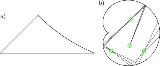
Abbildung 1: Two billiard systems: a) the desymmetrized diamond billiard; b) the cardioid billiard, with a fan of trajectories focusing in a “braid” of mutually conjugate points (marked by circles).

In semidispersing billiards, the boundary consists of locally concave and straight lines. For instance, the desymmetrized diamond billiard, see Fig. 1a, is surrounded by a part of a circle and by two straight lines. It can be seen as originating from a diamond-shaped billiard (the Sinai billiard with overlapping disks), cut into eight equal pieces.

The cardioid billiard has a heart-shaped boundary, defined by the equation $(q_{1}^{2}+q_{2}^{2}-q_{1})^{2}-(q_{1}^{2}+q_{2}^{2})=0$. The boundary is locally convex; hence the cardioid belongs to the family of focusing billiards. A particular characteristic of this family is the existence of conjugate points. A fan of trajectories (with an infinitesimal opening angle) starting from one point in configuration space may focus again in a second one after the next reflection. The latter point is called conjugate to the initial one. There may even be whole “braids” of mutually conjugate points, as in Fig. 1b.

4 Symbolic dynamics

One of the nice features of the billiards introduced is symbolic dynamics. In systems with symbolic dynamics, periodic orbits are fixed by certain sequences of numbers. For instance, in semidispersing billiards these numbers denote the segments of the boundary where the orbit is reflected [30, 32]. For the desymmetrized diamond billiard, there will be three symbols for the three parts of the boundary, see Fig. 2a, and the symbol sequence corresponding to an orbit will just enumerate all reflections inside that orbit. For each sequence of symbols, there is at most one orbit; sequences without an associated orbit are called “pruned”. Obviously, symbol sequences of periodic orbits are defined modulo cyclic permutations of their members.

Periodic orbits of the cardioid can be described in an alphabet of two symbols, representing the orbit segments between two reflections [31, 32]. “Clockwise” segments are denoted by $A$. More precisely, as sketched in Fig. 2b, the symbol $A$ refers to clockwise motion in the vicinity of the boundary, segments leading to a point just below the cusp, and everything in between. Similarly, “counter-clockwise” segments are labelled by $B$.

More generally, symbolic dynamics can be defined by introducing a Poincaré section, e.g., consisting of all phase-space points with configuration-space coordinates on the boundary of a billiard. This section is then divided into several regions, and we assign one symbol to each of them. The symbol sequence of an orbit now depends on the points of piercing through that section; for each piercing, the symbol of the corresponding region is added to the sequence. However, the symbolic dynamics thus defined will be useful only if there is (at most) one orbit per symbol sequence.

In time-reversal invariant systems, one can typically also define a time-reversal operation acting on symbol sequences. In the example of the desymmetrized diamond, time reversal simply means that the ordering of symbols is reversed. In the cardioid billiard, time reversal both inverts the order of symbols and interchanges $A\leftrightarrow B$.

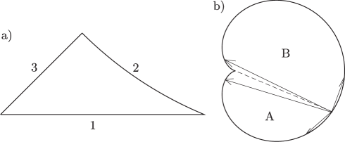
Abbildung 2: Symbolic dynamics: a) In the desymmetrized diamond, symbols label boundary segments 1,2, and 3; b) in the cardioid, $A$ denotes “clockwise” orbit segments and $B$ “counter-clockwise” ones, as explained in the text.

2 Level density à la Gutzwiller and Weyl

In the semiclassical limit, quantum spectra can be approximately determined from information about the pertaining classical dynamics. The level density $\rho(E)=\sum_{j}\delta(E-E_{j})$ of a bounded quantum system ($E_{j}$ denoting the energy levels) may be split into a local average $\overline{\rho}(E)$ and an oscillatory part $\rho_{\rm osc}(E)$ describing fluctuations around that average. As shown by Weyl, the smooth part $\overline{\rho}(E)$ is given by the number of Planck cells $(2\pi\hbar)^{f}$ inside the energy shell; we thus obtain

$$\overline{\rho}(E)\sim\frac{\Omega(E)}{(2\pi\hbar)^{f}},$$ (15)

with $\Omega(E)$ again denoting the volume of the energy shell.

On the other hand, the oscillatory contribution to the level density depends on the classical periodic orbits of the system in question. For the case of isolated periodic orbits, this relation was discovered by Gutzwiller; his results mainly cover hyperbolic systems (with all orbits isolated and unstable), but also exceptional dynamics with isolated stable orbits. Gutzwiller showed that $\rho_{\rm osc}(E)$ is given by a sum over periodic orbits $\gamma$

$$\rho_{\rm osc}(E)\sim\frac{1}{\pi\hbar}\operatorname{Re}\sum_{\gamma}A_{\gamma}{\rm e}^{{\rm i}S_{\gamma}/\hbar},$$ (16)

each orbit contributing with a phase determined by its classical (reduced) action $S_{\gamma}=\oint_{\gamma}{\bf p}\cdot d{\bf q}$ and with a stability “amplitude”

$$A_{\gamma}=\frac{T_{\gamma}^{\rm prim}}{\sqrt{|\det(M_{\gamma}-1)|}}{\rm e}^{-{\rm i}\mu_{\gamma}\frac{\pi}{2}}.$$ (17)

Here, $T_{\gamma}^{\rm prim}$ is the primitive period of $\gamma$; hence if $\gamma$ consists only of multiple repetitions of a shorter orbit, we have to use the period of the latter. Apart from the case of repetitions, $|A_{\gamma}|^{2}$ coincides with the factor ${\cal A}_{\gamma}^{2}$, see Eq. (11), appearing in the sum rule (12) of Hannay and Ozorio de Almeida and in the equidistribution theorem (14). Since among all orbits, such repetitions form a set of measure zero, we may safely replace ${\cal A}_{\gamma}^{2}\to|A_{\gamma}|^{2}$ in the sum rules (12) and (14).

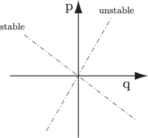
Abbildung 3: Stable and unstable directions, visualized by straight dash-dotted lines, in a Poincaré section ${\cal P}$ parametrized by configuration-space and momentum coordinates $q$ and $p$.

The so-called Maslov index $\mu_{\gamma}$ has an interesting geometrical interpretation [33], which will be exploited later. As in Section 1, let us consider a Poincaré section ${\cal P}$ orthogonal to the orbit in an arbitrary point on $\gamma$. For simplicity, we assume two degrees of freedoms. If we parametrize ${\cal P}$ by configuration-space and momentum coordinates $q$ and $p$, the stable and unstable directions can be visualized by straight lines through the origin, see Fig. 3. If we move ${\cal P}$ along the orbit, these lines will rotate around the origin, returning to their initial position after each half-rotation. Given that the orbit is periodic, they both have to come back to their initial position after one period. Hence, the number of (clockwise) half-rotations along the orbit is integer and will be referred to as the Maslov index $\mu_{\gamma}$ of that orbit.

We want to sketch the main ideas needed to derive (16). The level density may be obtained from the trace of the time evolution operator $\operatorname{Tr}\,\hat{U}(T)=\sum_{j}{\rm e}^{-{\rm i}E_{j}T/\hbar}$ as the imaginary part of the one-sided Fourier transform $\frac{\rm i}{\pi\hbar}\int_{0}^{\infty}dT\,{\rm e}^{{\rm i}Et/\hbar}\operatorname{Tr}\,\hat{U}(T)$ (hence the name “trace formula” for (16)). We now express the diagonal elements $\langle{\bf q}_{0}|\hat{U}(T)|{\bf q}_{0}\rangle$ as path integrals over trajectories closed in configuration space with ${\bf q}(0)={\bf q}(T)={\bf q}_{0}$, the integrand ${\rm e}^{{\rm i}F[{\bf q}(t)]/\hbar}$ depending on the (full) action $F[{\bf q}(t)]=\int_{0}^{T}L({\bf q}(t),\dot{\bf q}(t))dt$ of the trajectory in question. This path integral is evaluated in a stationary-phase approximation, leading to a sum over classical orbits which start and end at ${\bf q}_{0}$ and have stationary action, i.e., solve the canonical equations of motion. If we subsequently integrate over ${\bf q}_{0}$ and perform the Fourier transformation, further stationary-phase approximations lead to the sum (16) over orbits periodic in phase space, contributing with their reduced action $S[{\bf q}(t)]=F[{\bf q}(t)]-ET=\oint{\bf p}\cdot d{\bf q}$.

3 Universal spectral statistics

In the semiclassical limit, fully chaotic quantum systems display universal properties, only depending on their symmetries. One example stands out and will be the object of our investigation: According to the Bohigas-Giannoni-Schmit (BGS) conjecture put forward about two decades ago [5, 6], highly excited energy levels of generic fully chaotic systems have universal spectral statistics. As a preparation, we need to investigate the symmetries of classical and quantum dynamics, and show how to characterize the statistics of energy levels.

1 Symmetry classes

To bar unnecessary difficulties, we will consider only dynamics without conserved quantities; hence there may be no Hermitian observables $\hat{A}$ commuting with the Hamiltonian $\hat{H}$. In particular, this excludes any geometric symmetries, such as reflection symmetry.

The systems may, however, be invariant with respect to time reversal. Typically, if we traverse a trajectory with opposite sense, the momentum will change its sign. This defines the conventional time-reversal operator acting on phase-space coordinates ${\bf x}=({\bf q},{\bf p})$ as ${\cal T}({\bf q},{\bf p})=({\bf q},-{\bf p})$. A given classical dynamics is called conventionally time-reversal invariant if the Hamiltonian is even in the momentum, i.e., if $H({\bf q},-{\bf p})=H({\bf q},{\bf p})$. In this case each trajectory ${\bf x}(t)$ solving the canonical equations of motion yields a second solution via time reversal, given by ${\cal T}{\bf x}(-t)$.

For the quantum dynamics, conventional time reversal amounts to complex conjugation of the wavefunction ${\cal T}(\psi)=\psi^{*}$. A Hamiltonian is time-reversal invariant if it commutes with ${\cal T}$, i.e., if it is real (and thus symmetric). In this case, it is easy to show that each solution $\psi({\bf q},t)$ of the Schrödinger equation $\hat{H}\psi({\bf q},t)=i\hbar\partial_{t}\psi({\bf q},t)$ gives rise to a second one, namely ${\cal T}({\bf q},-t)=\psi^{*}({\bf q},-t)$.

A more general notion of time reversal includes operators ${\cal T}$ which are both antilinear and antiunitary. Hence, for all $a_{1},a_{2}\in\mathbb{C}$ and all wavefunctions $\psi_{1},\psi_{2}$, we must have

$${\cal T}(a_{1}\psi_{1}+a_{2}\psi_{2}) = a_{1}^{*}{\cal T}\psi_{1}+a_{2}^{*}{\cal T}\psi_{2},$$

$$\langle{\cal T}\psi_{1}|{\cal T}\psi_{2}\rangle = \langle\psi_{1}|\psi_{2}\rangle^{*}.$$ (18)

For example, ${\cal T}$ may refer to conventional time reversal, accompanied by a reflection in configuration space. Systems with non-conventional time-reversal invariance essentially show the same properties as conventionally time-reversal invariant ones, and can even be brought to conventional form by a suitable canonical transformation.

A time-reversal operator may square either to 1 or to $-1$, where the latter case is possible only for systems with spin. Hamiltonian dynamics can thus be divided into the three symmetry classes introduced by Wigner and Dyson:

• the unitary class containing systems without time-reversal invariance,

• the orthogonal class of dynamics invariant under a time-reversal operator ${\cal T}$ with ${\cal T}^{2}=1$,

• and the symplectic class of ${\cal T}$-invariant (spin) systems with ${\cal T}^{2}=-1$.

Since we expect universal behavior only for fully chaotic dynamics without conserved quantities, we restrict membership of the above three classes to only such systems.

Recently, Wigner’s and Dyson’s “threefold way” was extended by seven new classes [34] connected to further symmetries, such as symmetry with respect to charge conjugation. These new classes are of experimental relevance, e.g., for normal-metal/superconductor heterostructures and in quantum chromodynamics.

2 Spectral statistics

Level statistics can be characterized by the two-point correlation function of the level density, proportional to $\rho_{\rm osc}(E+\frac{\epsilon}{2})\rho_{\rm osc}(E-\frac{\epsilon}{2})$. To obtain a plottable function, two averages (to be denoted by $\langle\ldots\rangle$) are necessary, like over windows of the center energy $E$ and the energy difference $\epsilon$. Moreover, it is convenient to make the energy difference dimensionless by referral to the mean level spacing $\frac{1}{\overline{\rho}}$, setting $s\equiv\pi\overline{\rho}\epsilon$. We thus define the two-point correlator as

$$R(s)\equiv\left\langle\frac{\rho_{\rm osc}(E+\frac{s}{2\pi\overline{\rho}})\rho_{\rm osc}(E-\frac{s}{2\pi\overline{\rho}})}{\overline{\rho}(E)^{2}}\right\rangle\ =\left\langle\frac{\rho(E+\frac{s}{2\pi\overline{\rho}})\rho(E-\frac{s}{2\pi\overline{\rho}})}{\overline{\rho}(E)^{2}}\right\rangle-1\,,$$ (19)

where the last equality follows from $\langle\rho_{\rm osc}\rangle=0$.

The prime object of our investigation will be the Fourier transform of $R(s)$, the so-called spectral form factor

$$K(\tau)=\frac{1}{\pi}\int_{-\infty}^{\infty}ds\,e^{2{{\rm i}}s\tau}R(s)\,.$$ (20)

The variable $\tau>0$, conjugate to $s$, denotes the time measured in units of the Heisenberg time

$$T_{H}=2\pi\hbar\overline{\rho}(E)=\frac{\Omega(E)}{(2\pi\hbar)^{f-1}}.$$ (21)

By combining Eqs. (19-21), we may represent the form factor as

$$K(\tau)=\left\langle\int d\epsilon\,{\rm e}^{{\rm i}\epsilon\tau T_{H}/\hbar}\frac{\rho_{\rm osc}(E+\frac{\epsilon}{2})\rho_{\rm osc}(E-\frac{\epsilon}{2})}{\overline{\rho}(E)}\right\rangle\,,$$ (22)

where we have replaced the average over the energy difference by an average over a small window of $\tau$, and kept the average over $E$. Since the study of high-lying states justifies the semiclassical limit, we may take $\hbar\to 0,T_{H}\to\infty$, for fixed $\tau$.

Given full chaos, $K(\tau)$ is found to have a universal form, as obtained by averaging over certain ensembles of random matrices [1, 2, 3, 4]. Choosing an arbitrary orthonormal basis, the Hamiltonian may be written as an infinite matrix. For systems without symmetries (unitary class), we only know that this matrix must be Hermitian, whereas for time-reversal invariant dynamics with ${\cal T}^{2}=1$ (orthogonal class) it must be real and symmetric. Rather than considering an individual Hamiltonian, we now average over the ensembles of all Hermitian or real symmetric matrices, integrating over all independent matrix elements and taking the limit of infinite matrix dimension $N\to\infty$. The weight must be chosen invariant under transformations that leave these sets of matrices invariant; not surprisingly, these are orthogonal transformations for the orthogonal class and unitary transformations for the unitary class. To furthermore guarantee matrix elements to be uncorrelated, we need a Gaussian weight ${\cal A}\,{\rm e}^{-{\cal B}\operatorname{Tr}\,\hat{H}^{2}}$, ${\cal A},{\cal B}=\mbox{const}$. Hence we speak of the Gaussian Unitary and Orthogonal Ensembles (GUE and GOE); a Gaussian Symplectic Ensemble (GSE) may be defined similarly. For the three Gaussian ensembles, random-matrix averages yield the following predictions for the spectral form factor

$$K(\tau)=\begin{cases}\tau&\mbox{GUE,\ $\tau\leq 1$}\\ 1&\mbox{GUE,\ $\tau>1$}\\ 2\tau-\tau\ln(1+2\tau)=2\tau-2\tau^{2}+2\tau^{3}-\ldots&\mbox{GOE,\ $\tau\leq 1$}\\ 2-\tau\ln\frac{2\tau+1}{2\tau-1}&\mbox{GOE,\ $\tau>1$}\\ \frac{\tau}{2}-\frac{\tau}{4}\ln(1-\tau)=\frac{\tau}{2}+\frac{\tau^{2}}{4}+\frac{\tau^{3}}{8}+\ldots&\mbox{GSE,\ $\tau\leq 2$}\\ 1&\mbox{GSE,\ $\tau>2$;}\end{cases}$$ (23)

the $\tau$ expansions for the orthogonal and the symplectic case respectively converge for $0<\tau<\frac{1}{2}$ and $0<\tau<1$.

A further indicator of level statistics is the so-called level spacing distribution $P(s)$, i.e., the distribution of differences $s$ between neighboring energy levels, measured in units of the mean level spacing. Random-matrix theory (RMT) yields

$$P(s)\propto s^{\beta}{\rm e}^{-\alpha s^{2}}$$ (24)

with $\beta=2,1,4$ for the GUE, GOE, and GSE, respectively; the factor $\alpha$ depends on the symmetry class as well. Most importantly, $P(s)\to 0$ for $s\to 0$ implies the energy levels of chaotic systems have a tendency to repel each other.

According to the BGS conjecture, the level statistics of individual chaotic dynamics is faithful to the predictions, like (23) and (24), of the pertaining random-matrix ensembles. A proof of this conjecture, and even the precise assumptions required for a proof, have thus far remained a challenge. In the present thesis, we take up the challenge, and derive the small-$\tau$ expansion of $K(\tau)$ for individual systems; as our main assumptions, we employ ergodicity and hyperbolicity of the classical dynamics. Large $\tau$ will not be considered.

Our approach will be based on periodic-orbit theory, following previous work in [12, 13, 14, 15]. Earlier approaches followed different strategies. For example, in an ansatz known as parametric level dynamics [2], the quantum spectrum is modeled as a fictitious gas, with levels as particles; equilibration then gives rise to universal statistics. Field-theoretical methods were employed in a non-perturbative setting in [8], and perturbatively in [9, 10, 11].

4 Diagonal approximation

Using Gutzwiller’s trace formula, the form factor is expressed as a double sum over orbits $\gamma$, $\gamma^{\prime}$,

$$K(\tau)\sim\frac{1}{T_{H}}\left\langle\sum_{\gamma,\gamma^{\prime}}A_{\gamma}A_{\gamma^{\prime}}^{*}{\rm e}^{{\rm i}(S_{\gamma}-S_{\gamma^{\prime}})/\hbar}\delta\left(\tau T_{H}-\frac{T_{\gamma}+T_{\gamma^{\prime}}}{2}\right)\right\rangle\,.$$ (25)

To obtain this expression, we have to combine (16) and (22), expand the action to linear order $S_{\gamma}(E\pm\frac{\epsilon}{2})\approx S_{\gamma}(E)\pm T_{\gamma}(E)\frac{\epsilon}{2}$ and leave out oscillatory terms $\propto\exp\left(\pm\frac{{\rm i}}{\hbar}(S_{\gamma}+S_{\gamma^{\prime}})\right)$.

Most importantly, (25) implies that for $\hbar\to 0$, only families of orbit pairs with small action difference $|S_{\gamma}-S_{\gamma^{\prime}}|\hbox{$<\kern-10.00002pt{\lower 4.30554pt\hbox{$\sim$}}$\thinspace}\hbar$ can give a systematic contribution to the form factor. For all others, the phase in (25) oscillates rapidly, and the contribution is killed by the averages indicated. Correlations of quantum spectra are thus related to correlations among the actions of classical orbits [13].

The simplest approximation is to keep only “diagonal” pairs of coinciding ($\gamma^{\prime}=\gamma$) and, for time $\cal T$-invariant dynamics, mutually time-reversed ($\gamma^{\prime}={\cal T}\gamma$) orbits, which obviously are identical in action. Indeed, Berry [12] showed that these pairs give rise to the leading term in the power series of $K(\tau)$. Restricting ourselves to diagonal pairs, we obtain the single sum

$$K_{\rm diag}(\tau)=\frac{\kappa}{T_{H}}\left\langle\sum_{\gamma}|A_{\gamma}|^{2}\delta(\tau T_{H}-T_{\gamma})\right\rangle,$$ (26)

with $\kappa=1$ in the unitary case. For ${\cal T}$-invariant dynamics belonging to the orthogonal class, we also have to account for mutually time-reversed orbits; hence we have to multiply with $\kappa=2$. Using the sum rule of Hannay and Ozorio de Almeida [25], see Eq. (12), the sum in Eq. (26) is easily evaluated to give

$$K_{\rm diag}(\tau)=\kappa\tau,$$ (27)

as predicted by RMT; compare (23).

One may expect that higher-order contributions to the form factor arise from further families of orbit pairs. Indeed, using the predictions for $K(\tau)$, Argaman et al. [13] derived a random-matrix expression for classical correlations between actions of periodic orbits. For several systems, the existence of additional correlations could be confirmed numerically, motivating further studies in [35, 36, 37, 38, 39]. The orbit pairs giving rise to the $\tau^{2}$ contribution to the spectral form factor were recently identified by Sieber and Richter. They will be the subject of the following Chapter.

5 Summary

In this chapter, we introduced basic notions of classical and quantum chaos. Classically, fully chaotic systems are characterized by hyperbolicity and ergodicity. Due to hyperbolicity, small phase-space separations may be decomposed into an unstable component (growing exponentially in time) and a stable component (shrinking exponentially in time). Ergodicity implies that long trajectories uniformly fill the energy shell. Prominent examples are chaotic billiards, whose orbits may be conveniently described by sequences of symbols.

On the quantum-mechanical side, energy levels of fully chaotic systems have universal statistics, characterized for example by the spectral form factor $K(\tau)$, the Fourier transform of the two-point correlation function of the level density. According to the so-called BGS conjecture, the form factor depends only on whether the system in question has no time-reversal (${\cal T}$) invariance (unitary class), or is ${\cal T}$ invariant with either ${\cal T}^{2}=1$ (orthogonal class) or ${\cal T}^{2}=-1$ (symplectic class); $K(\tau)$ is found to agree with averages over the pertaining Gaussian ensembles of random matrices.

To explain the universal statistics of quantum spectra, we will employ results from classical chaos. Hyperbolicity allows to represent the fluctuating part of the level density as a sum over periodic orbits, with an amplitude depending on their classical stability and a phase involving their classical action (divided by $\hbar$). The form factor may thus be written as a double sum over periodic orbits, the phase of each pair given by the difference between actions (again divided by $\hbar$). As shown by Berry, the leading contribution to the $\tau$ expansion of $K(\tau)$ originates from pairs of orbits identical up to time-reversal.

Kapitel 2 $\tau^{2}$ contribution to the spectral form factor

1 Preliminaries

The family of orbit pairs responsible for the next-to-leading order of $K(\tau)$ was identified in Sieber’s and Richter’s seminal papers [14, 15] for a homogeneously hyperbolic system, the so-called Hadamard-Gutzwiller model (geodesic motion on a tesselated surface of negative curvature with genus 2). In each Sieber/Richter pair, one orbit narrowly avoids one of the many small-angle self-crossings of its partner; see Fig. 1 or Fig. 1.

We have already sketched the phase-space description of these orbit pairs. Both orbits $\gamma$ and $\gamma^{\prime}$ contain an “encounter” of two almost time-reversed orbit stretches. These encounter stretches divide the remainder of $\gamma$ and $\gamma^{\prime}$ into two “loops”. The two orbits are distinguished only by different connections inside the encounter. The partner $\gamma^{\prime}$ almost coincides with $\gamma$ in one loop, whereas it is nearly time-reversed with respect to $\gamma$ in the other loop. Sieber/Richter pairs may exist only in time-reversal invariant systems, since it must be possible to traverse an orbit loop with opposite sense of motion.

For systems with symbolic dynamics, Sieber/Richter pairs can be characterized by their symbol sequences. To do so, we assign a symbol sequence to each encounter stretch and each loop. Note that two close stretches or loops have the same symbol string since they will, e.g., bounce from the same parts of the boundary with the same ordering. Likewise, two approximately time-reversed stretches or loops are described by exactly time-reversed sequences. Thus, the two almost time-reversed stretches will have symbol sequences ${\cal E}$ and $\bar{{\cal E}}$, the overbar denoting time reversal. If we label the intervening loops by sequences ${\cal L}$ and ${\cal R}$, the whole orbit $\gamma$ will be described by the sequence ${\cal L}{\cal E}{\cal R}\bar{{\cal E}}$. The partner $\gamma^{\prime}$ must have the symbol string of one loop, say ${\cal R}$, reverted in time; the overall sequence will thus read $\gamma^{\prime}={\cal L}{\cal E}\bar{{\cal R}}\bar{{\cal E}}$ [17, 18, 40].

To show that the contribution of these orbit pairs agrees with the second term in the power series of the GOE form factor, $-2\tau^{2}$, two key ingredients are needed. First, Sieber and Richter showed that the action difference between the two partner orbits is determined by the crossing angle $\epsilon$ as $\Delta S\propto\frac{\epsilon^{2}}{2}+O(\epsilon^{3})$. Second, they investigated the statistics of self-crossings. The density of crossing angles contains a term logarithmic in $\epsilon$, which (although of subleading order in the orbit period) is crucial for spectral universality. Upon integrating over $\epsilon$, the latter term indeed gives rise to the anticipated contribution $-2\tau^{2}$.

This result was extended to general fully chaotic two-freedom systems in [18], connecting the treatment of self-crossings in configuration space with an analysis of the invariant manifolds in phase space. Sieber’s and Richter’s approach was subsequently reformulated purely in terms of phase-space coordinates by Spehner [23] and by Turek and Richter [24]. This formulation could, in an improved version, also be extended to systems with more than two degrees of freedom, as shown in a joint publication with these authors [21].

In contrast to the historical development, we here want to start with a treatment in terms of phase-space separations since that language will also be used when deriving higher-order contributions to the spectral form factor. The results for configuration-space crossings of [14, 15] and [18] will be reviewed in Appendix 8. That Appendix will also contain numerical investigations on billiards and more rigorous results on the Hadamard-Gutzwiller model, which are easier explained in the language of crossings.

Most of the reasoning in this and the following Chapters applies to general fully chaotic dynamics. For complete generality, just two points are missing: First, when showing that certain terms do not contribute to the form factor, we assume “homogeneously” hyperbolic dynamics, i.e., Lyapunov exponents of all orbits (and local stretching rates of all phase-space points) coinciding. The necessary modifications for general hyperbolic systems will be presented in Appendix 10.A, for all orders of $K(\tau)$. Second, for simplicity we restrict ourselves to systems with $f=2$ degrees of freedom. The results carry over to $f>2$ if we read the stable and unstable coordinates $s$, $u$ as $(f-1)$-dimensional vectors; the resulting changes will be listed in Appendix 10.B.

2 Encounters

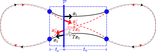
Abbildung 1: Configuration-space sketch of a Sieber/Richter pair of orbits $\gamma$ (full line) and $\gamma^{\prime}$ (dashed line). The orbits differ by their connections inside the encounter (thick lines, marked by a box). Both orbits pierce twice through a Poincaré section ${\cal P}$ inside the encounter; the piercing points ${\bf x}_{1},{\bf x}_{2},{\bf x}_{1}^{\prime},{\bf x}_{2}^{\prime}$ and the time-reversed piercing points ${\cal T}{\bf x}_{2},{\cal T}{\bf x}_{2}^{\prime}$ are marked by arrows pointing in the direction of motion. The times $t_{u}$ and $t_{s}$ are the durations of the “head” and “tail” of the encounter.

We will describe encounters by phase-space coordinates. To do so, we introduce a Poincaré surface of section ${\cal P}$ orthogonal to the orbit at an arbitrary phase-space point ${\bf x}_{1}$ (passed at time $t_{1}$) inside one of the encounter stretches, as in Fig. 1. The exact location of ${\cal P}$ inside the encounter is not important. The second stretch pierces through ${\cal P}$ at a time $t_{2}$ in an almost time-reversed point ${\bf x}_{2}$. The small difference ${\cal T}{\bf x}_{2}-{\bf x}_{1}$ can be decomposed in terms of the stable and unstable directions at ${\bf x}_{1}$,

$${\cal T}{\bf x}_{2}-{\bf x}_{1}=s{\bf e}^{s}({\bf x}_{1})+u{\bf e}^{u}({\bf x}_{1})\;.$$ (1)

The stable and unstable components $s$, $u$ depend on the location ${\bf x}_{1}$ of the Poincaré section ${\cal P}$ chosen within the encounter. If we shift ${\cal P}$ through the encounter, the stable components will asymptotically decrease and the unstable components will asymptotically increase with growing $t_{1}$, according to Eqs. (1) and (4).

We can now refine our definition of an encounter. To guarantee that both stretches are almost mutually time-reversed, we demand both $|s|$ and $|u|$ to be smaller than a constant $c$. The bound $c$ must be chosen small enough for the motion around the two orbit stretches to allow for the mutually linearized treatment (1); however, the exact value of $c$ is not important for the following considerations.

By definition, the encounter begins when the stable component $|s|$ falls below $c$, and ends when the unstable component $|u|$ reaches $c$. The duration of an encounter is thus obtained by summing the durations of the “head” of the encounter (i.e., the time $t_{u}$ until the unstable component $|u|$ reaches $c$) and its “tail” (i.e., the time $t_{s}$ passed since the stable components $|s|$ has fallen below $c$) as depicted in Fig. 1. Given that the unstable components grow exponentially in time, we have $|u|{\rm e}^{\lambda t_{u}}\sim c$ and thus

$$t_{u}\sim\frac{1}{\lambda}\ln\frac{c}{|u|}.$$ (2)

Similarly, the “tail” has the duration

$$t_{s}\sim\frac{1}{\lambda}\ln\frac{c}{|s|}.$$ (3)

The overall duration of the encounter is thus given by

$$t_{\rm enc}=t_{s}+t_{u}\sim\frac{1}{\lambda}\ln\frac{c^{2}}{|su|}\,.$$ (4)

Reassuringly, (1) guarantees that the product $su$ and hence the duration $t_{\rm enc}$ remain invariant if the Poincaré section ${\cal P}$ is shifted through the encounter.

Note that we here described the local divergence inside the encounter through the global Lyapunov of the system $\lambda$. For inhomogeneously hyperbolic systems, this is only an approximation (to be avoided in Appendix 10.A), but rather accurate for typical long encounters, which can be expected to explore the energy shell approximately uniformly.

3 Partner orbits

Each encounter of two antiparallel stretches inside a periodic orbit $\gamma$ gives rise to a partner orbit $\gamma^{\prime}$. The partner $\gamma^{\prime}$ is distinguished from $\gamma$ by differently connecting the “ports” (i.e., the initial and final points) of the encounter stretches, marked by dots in Fig. 1. Moreover, $\gamma^{\prime}$ has one, say, the “right” loop reversed in time.

1 Partner piercings

The partner $\gamma^{\prime}$ also pierces through the Poincaré section ${\cal P}$ in two almost mutually time-reversed phase-space points ${\bf x}_{1}^{\prime}$ and ${\bf x}_{2}^{\prime}$, with ${\bf x}_{1}^{\prime}\approx{\cal T}{\bf x}_{2}^{\prime}\approx{\bf x}_{1}$. These piercings are determined by those of $\gamma$.

Let us first consider ${\bf x}_{1}^{\prime}$. The stretches passing through ${\bf x}_{1}^{\prime}$ and ${\cal T}{\bf x}_{2}$ lead to (practically) the same port. Two trajectories starting at ${\bf x}_{1}^{\prime}$ and ${\cal T}{\bf x}_{2}$ thus approach each other for a long time, at least until the end of the encounter and half-way through the subsequent loop; in fact we shall see that the durations of the relevant encounters diverge in the limit $\hbar\to 0$. Hence, the difference between ${\bf x}_{1}^{\prime}$ and ${\cal T}{\bf x}_{2}$ must be close to the stable manifold, and their unstable coordinates practically coincide. Similarly, the stretches passing through ${\bf x}_{1}^{\prime}$ and ${\bf x}_{1}$ start from the same port and thus approach for large negative times. Hence, their difference is close to the unstable direction, and the corresponding stable coordinates coincide. We can draw the location of the corresponding piercing points in our Poincaré section, spanned by stable and unstable directions (Fig. 2). If we choose ${\bf x}_{1}$ as the origin of that section, ${\cal T}{\bf x}_{2}$ will have the stable coordinate $s$ and the unstable coordinate $u$. The piercing point ${\bf x}_{1}^{\prime}$ must have the same stable coordinate as ${\bf x}_{1}$ and the same unstable coordinate as ${\cal T}{\bf x}_{2}$, i.e.,

$$s_{1}^{\prime}=0,\;u_{1}^{\prime}=u.$$ (5a)

Similarly, one can show that $${\cal T}{\bf x}_{2}^{\prime}$$ has the coordinates

$$s_{2}^{\prime}=s,\;u_{2}^{\prime}=0.$$ (5b)

Thus, the piercings of $\gamma$ and $\gamma^{\prime}$ together span a parallelogram in ${\cal P}$ [41] (depicted as a rectangle in Fig. 2). The uniqueness of (5) implies that there is exactly one partner orbit per encounter.

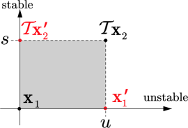
Abbildung 2: Piercing points of the original orbit $\gamma$ and its partner $\gamma^{\prime}$ through a Poincaré section, parametrized by stable and unstable coordinates. The area of the rectangle coincides with the action difference $\Delta S$. (Note that the Sieber/Richter pair in Fig. 1 has an action difference $\Delta S=S_{\gamma}-S_{\gamma^{\prime}}<0$ and thus either $s$ or $u$ negative.)

2 Action difference

We can now determine the difference between the actions of the two partner orbits. Generalizing the results for configuration-space crossings in [14, 15, 18], we will show that the action difference is just the symplectic area of the rectangle in Fig. 2 [23, 24]. Consider two segments of the encounter stretches leading from the port on the upper left side in Fig. 1 to the piercing point ${\bf x}_{1}$ of $\gamma$, and to the piercing point ${\bf x}_{1}^{\prime}$ of $\gamma^{\prime}$, respectively. Since the action variation brought about by a shift $d{\bf q}$ of the final coordinate is ${\bf p}\cdot d{\bf q}$, the action difference between the two segments will be given by $\Delta S^{(1)}=\int_{{\bf x}_{1}^{\prime}}^{{\bf x}_{1}}{\bf p}\cdot d{\bf q}$. The integration line may be chosen to lie in the Poincaré section; then it coincides with the unstable axis. Repeating the same reasoning for the remaining segments, we obtain the overall action difference $\Delta S\equiv S_{\gamma}-S_{\gamma^{\prime}}$ as the line integral $\Delta S=\oint{\bf p}\cdot d{\bf q}$ along the contour of the parallelogram ${\bf x}^{\prime}_{1}\to{\bf x}_{1}\to{\cal T}{\bf x}^{\prime}_{2}\to{\cal T}{\bf x}_{2}\to{\bf x}^{\prime}_{1}$, spanned by ${\bf x}_{1}^{\prime}-{\bf x}_{1}={u}{\bf e}^{u}({\bf x}_{1})$ and ${\cal T}{\bf x}_{2}^{\prime}-{\bf x}_{1}={s}{\bf e}^{s}({\bf x}_{1})$. This integral indeed gives the symplectic area

$$\Delta S={u}{\bf e}^{u}({\bf x}_{1})\land{s}{\bf e}^{s}({\bf x}_{1})={s}{u}\,,$$ (6)

where we used the normalization in Eq. (7). If the above parallelogram is depicted as a rectangle, like in Fig. 2, the action difference can simply be interpreted as a geometric area.

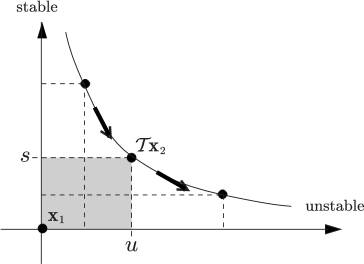
Abbildung 3: As ${\cal P}$ is shifted through the encounter, the piercing point ${\cal T}{\bf x}_{2}$ travels on a hyperbola with $\Delta S=su$ constant.

We have already revealed $su$ as independent of the location of ${\cal P}$. If we shift ${\cal P}$ through the encounter, ${\cal T}{\bf x}_{2}$ will travel on a hyperbola with $\Delta S=su$ fixed, with unstable coordinates growing and stable coordinates shrinking asymptotically; see Fig. 3. As ${\cal T}{\bf x}_{2}$ moves, the rectangle in ${\cal P}$ is deformed, but its symplectic area is conserved (as it should be, given a Hamiltonian flow).

At this point, we can finally appreciate that the encounters relevant for spectral universality have a duration of the order of the Ehrenfest time. The form factor is determined by orbit pairs with an action difference $\Delta S=su$ of order $\hbar$; hence indeed $t_{\rm enc}\sim\frac{1}{\lambda}\ln\frac{c^{2}}{|su|}=\frac{1}{\lambda}\ln\frac{c^{2}}{|\Delta S|}\sim\frac{1}{\lambda}\ln\frac{c^{2}}{\hbar}$.

3 Stability amplitudes

It remains to be shown that the relative difference between the stability amplitudes (see (11) and (17)) of $\gamma$,

$$A_{\gamma}=\frac{T_{\gamma}^{\rm prim}}{2\sinh\frac{\lambda_{\gamma}T_{\gamma}}{2}}{\rm e}^{-{\rm i}\mu_{\gamma}\frac{\pi}{2}},$$ (7)

and $\gamma^{\prime}$ vanishes as the stable and unstable separations inside the encounter go to zero.

First, we want to demonstrate that both orbits have the same Maslov index. We use the geometrical interpretation of the Maslov index introduced in Section 2: As the Poincaré section ${\cal P}$ is shifted along the orbit, the stable and unstable manifolds rotate around the origin, relative to the configuration-space and momentum axes. The Maslov index of a periodic orbit counts the number of clockwise half-rotations. For our argument, we also define a Maslov index for non-periodic pieces of trajectory, as the sum of rotation angles of the stable and the unstable manifold, divided by $2\pi$. The Maslov index thus defined is invariant under time reversal. Obviously, time reversal leaves the absolute value of a rotation angle invariant. The same is true for the sense of rotation, since time reversal inverts the motion on the Poincaré section in direction (turning a clockwise rotation into a counter-clockwise one and vice versa), but also changes the sign of the momentum (turning the sense of rotation back to the original one). In addition, time reversal exchanges the stable and unstable manifolds, which also cannot affect the sum of their rotation angles. Thus, the Maslov index is time-reversal invariant. (An alternative proof for the Maslov index of a periodic orbit is given in [42].)

The Maslov index of $\gamma$ is now obtained by summing the Maslov indices of the encounter stretches and loops. To obtain a partner orbit, we invert the direction of motion on one loop, leaving $\mu_{\gamma}$ invariant, and reconnect the orbit inside the encounter. The latter reconnections could at most lead to a small change of $\mu_{\gamma}$, vanishing for phase-space separations going to zero. Given that $\mu_{\gamma}$ and $\mu_{\gamma^{\prime}}$ have to be integer, reconnections cannot affect the Maslov index at all; hence indeed $\mu_{\gamma^{\prime}}=\mu_{\gamma}$.

Trivially, the primitive periods $T_{\gamma}^{\rm prim}$ and $T_{\gamma^{\prime}}^{\rm prim}$ approximately coincide, since the duration of orbit loops and encounter stretches is invariant under time reversal, and only slightly changed by reconnections. (Incidentally, for billiards the periods of $\gamma$ and $\gamma^{\prime}$ are proportional to the almost coinciding actions.)

The Lyapunov exponents $\lambda_{\gamma}$ and $\lambda_{\gamma^{\prime}}$ exactly coincide for homogeneously hyperbolic dynamics. For inhomogeneously hyperbolic systems, recall that the Lyapunov exponent $\lambda_{\gamma}$ is obtained by averaging the local stretching rate $\chi({\bf x}(t))$ over the orbit $\gamma$, i.e., $\lambda_{\gamma}T_{\gamma}=\int_{0}^{T_{\gamma}}dt\,\chi({\bf x}(t))$. In similar vein as above, time reversal of an orbit loop leaves $\lambda_{\gamma}T_{\gamma}$ unchanged, since $\chi({\bf x}(t))$ is time-reversal invariant. Reconnections inside the encounter may only lead to a small change, vanishing for $s,u\to 0$. Therefore, we indeed have $A_{\gamma^{\prime}}\approx A_{\gamma}$.

In contrast to the action difference, the difference between stability amplitudes or periods will never be referred to a small quantum scale. Since the relative differences between the amplitudes and periods of both partner orbits are small, we replace $A_{\gamma^{\prime}}\to A_{\gamma}$, $T_{\gamma^{\prime}}\to T_{\gamma}$. A rigorous justification of these approximations can be given for the Hadamard-Gutzwiller model, where the small difference between $A_{\gamma^{\prime}}$ and $A_{\gamma}$ can be evaluated analytically; see Appendix 8.C.

4 Necessity of non-vanishing loops

It is important to consider only encounters with stretches separated by non-vanishing loops. Only for such encounters, the two stretches will begin and end in four different ports, and reconnections between these ports give rise to a partner orbit. To be certain, we shall check in the following Subsection that our prescription for determining partner orbits cannot be extended to work in case of missing loops. Afterwards, we will formulate the condition of non-vanishing loops as a restriction on the piercing times $t_{1}$ and $t_{2}$.

1 Almost self-retracing encounters

How do we have to imagine an encounter without an external loop? If, say, the right loop in Fig. 1 is shrunk away, we will obtain an encounter as depicted in Fig. 4a. Somewhere within the encounter the orbit undergoes a nearly self-retracing reflection from a hard wall. After the reflection, the particle will for some time travel close to the pre-collision trajectory, such that technically an encounter of two antiparallel orbit pieces is formed. In some systems, such as the Hadamard-Gutzwiller model, reflections like this never take place, because there are no reflecting walls. In contrast, almost self-retracing encounters appear frequently in billiards, see Fig. 4b-c for two examples. Since there are only two ports, the encounter effectively has to be considered as one single stretch folded back upon reflection, and no partner can be obtained by reconnecting the two ports.

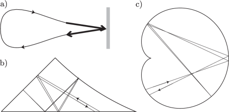
Abbildung 4: Almost self-retracing encounters: a) schematic sketch, b) example for the desymmetrized diamond billiard, c) example for the cardioid billiard.

To verify this intuitive picture, let us first consider systems with symbolic dynamics. The symbol sequences of the two partner orbits $\gamma={\cal L}{\cal E}{\cal R}\bar{{\cal E}}$, $\gamma^{\prime}={\cal L}{\cal E}\bar{{\cal R}}\bar{{\cal E}}$ turn out equal if the right loop with symbol sequence ${\cal R}$ is absent. Since pairs of identical (or mutually time-reversed) orbits are already included in the diagonal approximation, encounters without intervening loops give no off-diagonal contribution to the form factor.

To generalize this result to systems without symbolic dynamics, we first need to find an equation for the piercing points of the partner orbit $\gamma^{\prime}$ which remains valid even in absence of intervening loops. Let us again consider a Poincaré section ${\cal P}$ placed somewhere inside the encounter. This section divides the orbit into two parts (respectively containing the left and right loops, if present, and the “tail” and “head” of the encounter) whose stability matrices will be denoted by $L$ and $R$. Note that we do not require these orbit parts to be long. We assume that $\gamma^{\prime}$ approximately follows the “left” part of $\gamma$ in the same direction, and the “right” part with opposite direction. Clearly, this generalizes our previous prescription for finding partners: Rather than reverting one loop in time and changing connections between ports, we revert one orbit part; to obtain a classical periodic orbit, we then must change connections between the ends of the two orbit parts, and slightly deform the resulting trajectory. As in Fig. 1, the piercings of $\gamma$ and $\gamma^{\prime}$ will be denoted by ${\bf x}_{1}$, ${\bf x}_{2}$, ${\bf x}_{1}^{\prime}$, and ${\bf x}_{2}^{\prime}$. Since $\gamma$ and $\gamma^{\prime}$ are close in the left part leading from ${\bf x}_{2}$ to ${\bf x}_{1}$, we may linearize

$${\bf x}_{1}^{\prime}-{\bf x}_{1}=L({\bf x}_{2}^{\prime}-{\bf x}_{2}).$$ (8a)

The two orbits are almost mutually time-reversed in the right part, leading from $${\bf x}_{1} {\bf x}_{2} \gamma {\cal T}{\bf x}_{2} {\cal T}{\bf x}_{1} \gamma {\bf x}_{1}^{\prime} {\bf x}_{2}^{\prime} \gamma^{\prime} R^{\cal T}={\cal T}R^{-1}{\cal T}$$ to in . The time-reversed of that part leads from to in , and from to in ; it has the stability matrix . We thus obtain

$${\bf x}_{2}^{\prime}-{\cal T}{\bf x}_{1}=R^{\cal T}({\bf x}_{1}^{\prime}-{\cal T}{\bf x}_{2}).$$ (8b)

With $\delta{\bf x}_{1}={\bf x}_{1}^{\prime}-{\bf x}_{1}$, $\delta{\bf x}_{2}={\bf x}_{2}^{\prime}-{\bf x}_{2}$, $\delta{\bf x}={\cal T}{\bf x}_{2}-{\bf x}_{1}$, (8) simplifies to

$$\delta{\bf x}_{1} = L\delta{\bf x}_{2}$$

$$\delta{\bf x}_{2}+{\cal T}\delta{\bf x} = R^{\cal T}(\delta{\bf x}_{1}-\delta{\bf x}).$$ (9)

This system of equations uniquely determines the partner orbit $\gamma^{\prime}$. If the encounter stretches are separated by intervening loops, Eq. (9) will entail the solution (5) derived previously.

In contrast, if e.g. the “right” loop is absent, the right orbit part will remain inside the encounter for its whole duration. The phase-space separations inside that part may thus be followed in a linear approximation. We may, for instance, linearize the equations of motion around the trajectory leading from ${\cal T}{\bf x}_{2}$ to ${\cal T}{\bf x}_{1}$, with the stability matrix $R^{\cal T}$. During the same time, the piercing point ${\bf x}_{1}$ is carried into ${\bf x}_{2}$. Linearizing with the help of $R^{\cal T}$, we obtain (up to quadratic order in ${\cal T}{\bf x}_{2}-{\bf x}_{1}$)

$${\bf x}_{2}-{\cal T}{\bf x}_{1}=R^{\cal T}({\bf x}_{1}-{\cal T}{\bf x}_{2})$$ (10)

or, equivalently,

$${\cal T}\delta{\bf x}=-R^{\cal T}\delta{\bf x}.$$ (11)

Inserting the latter result into the second equation in (9), we see that (9) has the trivial solution $\delta{\bf x}_{1}=\delta{\bf x}_{2}=0$. Thus, the “partner” with time-reversed right loop coincides with the initial orbit. Conversely, if the left loop were absent, the corresponding “partner” would coincide with the time-reversed of the initial orbit. Again, we see that almost self-retracing encounters do not yield off-diagonal orbit pairs and therefore do not contribute to the spectral form factor.

2 Minimal distances

To give rise to a partner orbit, two encounter stretches need to be separated by intervening loops. Such loops exist if the times $t_{1}$ and $t_{2}$ (when the stretches pass through the section ${\cal P}$) observe certain minimal distances. To show this, we first have to fix notation. The times $t_{1}$ and $t_{2}$ are well defined only modulo the period of the orbit $T_{\gamma}$. In the sequel, it will be convenient to take $0<t_{1}<T_{\gamma}$ and $t_{1}<t_{2}<t_{1}+T_{\gamma}$.

To allow for a non-vanishing loop, the orbit part to the right of ${\cal P}$ (leading from $t_{1}$ to $t_{2}$) must exceed twice the duration of the head of the encounter. Only then it is long enough to contain (i) the head of the first encounter stretch with duration $t_{u}$, (ii) a loop of positive duration, and (iii) a piece of the second stretch again with duration $t_{u}$. Hence we have to demand that

$$t_{1}+2t_{u}<t_{2}$$ (12)

Similarly, the orbit part to the left of ${\cal P}$ (from $t_{2}$ to $t_{1}+T_{\gamma}$) must be longer than $2t_{s}$, to leave time for two traversals of the “tail” of the encounter, separated by a non-vanishing loop. We thus need to have

$$t_{2}<t_{1}+T_{\gamma}-2t_{s}$$ (13)

Altogether (12) and (13) imply that the time interval accessible to the second piercing is given by

$$(t_{1}+T_{\gamma}-2t_{s})-(t_{1}+2t_{u})=T_{\gamma}-2(t_{s}+t_{u})=T_{\gamma}-2t_{\rm enc};$$ (14)

i.e., it is reduced by the overall duration of both encounter stretches, $2t_{\rm enc}$.

5 Statistics of encounters

To determine the contribution of Sieber/Richter pairs to the spectral form factor, we need to count orbit pairs and thus encounters. More precisely, we have to determine the average number $P_{T}(\Delta S)d\Delta S$ of encounters inside orbits $\gamma$ with period $T$ leading to Sieber/Richter partners $\gamma^{\prime}$ with action difference $S_{\gamma}-S_{\gamma^{\prime}}$ inside $(\Delta S,\Delta S+d\Delta S)$. Given that the contribution of each orbit pair is proportional to $|A_{\gamma}|^{2}$, $P_{T}(\Delta S)$ has to be understood as averaged over the ensemble of all $\gamma$ with periods inside a time window around $T$, weighted with $|A_{\gamma}|^{2}$.

To evaluate $P_{T}(\Delta S)$, we introduce an auxiliary density $w_{T}(s,u)$ of stable and unstable separations inside encounters. Recall that these separations depend on the location of our Poincaré section. The density $w_{T}(s,u)$ will be normalized to guarantee that after integration over $s$ and $u$ each encounter is counted exactly once. Hence, we have to demand that

$$P_{T}(\Delta S)=\int_{-c}^{c}dsdu\,w_{T}(s,u)\delta(\Delta S-su).$$ (15)

To establish $w_{T}(s,u)$, we need only two ingredients: ergodicity and the necessity of having encounter stretches separated by non-vanishing loops. Note that even though individual periodic orbits need not be ergodic, the equidistribution theorem (Subsection 2) allows to invoke ergodicity when averaging over the ensembles of orbits introduced above.

Let us first fix one location of the section ${\cal P}$, at a point ${\bf x}_{1}$ (passed at time $t_{1}$) somewhere along the orbit. We now have to count all further piercings through this section in phase-space points ${\bf x}_{2}$ (passed at times $t_{2}$) almost time-reversed with respect to ${\bf x}_{1}$. Each of these piercing points will correspond to a different encounter, with ${\bf x}_{1}$ forming part of one stretch, and ${\bf x}_{2}$ belonging to the other one. Due to ergodicity, the expected number of piercings at times inside $(t_{2},t_{2}+dt_{2})$ with stable and unstable components of ${\cal T}{\bf x}_{2}-{\bf x}_{1}$ in intervals $(s,s+ds)$ and $(u,u+du)$ is given by the Liouville measure, expressed in terms of times and stable and unstable coordinates (see Subsection 2)

$$\frac{1}{\Omega}dsdudt_{2},$$ (16)

$\Omega$ denoting the volume of the energy shell.

The total number of piercing points inside intervals $ds$ and $du$ on our Poincaré section is obtained by integration over $t_{2}$. To guarantee that the encounter stretches are separated by intervening loops we have to restrict ourselves to $t_{1}+2t_{u}<t_{2}<t_{1}+T-2t_{s}$, i.e., an interval of width $T-2t_{\rm enc}$. Since the integrand is independent of $t_{2}$, the resulting density of piercing through one section is simply given by

$$\frac{1}{\Omega}(T-2t_{\rm enc}).$$ (17)

We have to keep into account all encounters along the orbit in question, and hence all possible Poincaré sections. Given that ${\cal P}$ is placed at a point ${\bf x}_{1}$, passed at time $t_{1}$, we thus have to integrate over all possible piercing times $0<t_{1}<T$, leading to a factor $T$. Note that ${\cal P}$ may be moved freely throughout each encounter without changing the partner orbit. Hence, when integrating over $t_{1}$ each encounter is counted for a time $t_{\rm enc}$. To avoid weighting each encounter with its duration, we have to divide out $t_{\rm enc}$.

Still, each encounter is counted twice, since any of the two encounter stretches may be considered as “the first”. Both choices give separate contributions to the above integrals. Dividing out 2, the desired density $w_{T}(s,u)$ is finally obtained as

$$w_{T}(s,u)=\frac{T(T-2t_{\rm enc}(s,u))}{2\Omega t_{\rm enc}(s,u)}.$$ (18)

We need to discuss two small corrections to (18). First, for loops shorter than a classical relaxation time $t_{\rm cl}$ describing the decay of correlations, the two piercings ${\bf x}_{1}$ and ${\bf x}_{2}$ will be correlated, leading to corrections to the piercing probability (16) and thus to (17) and (18). However, these corrections are negligible for $\hbar\to 0$, when $t_{\rm cl}$ vanishes compared to $T\sim T_{H}$ and $t_{\rm enc}\sim T_{E}$. Second, for inhomogeneously hyperbolic systems, the formula (4) used for the encounter duration $t_{\rm enc}(s,u)$ is only an approximation. We shall see in Appendix 10.A that the contribution to the form factor remains unaffected if we avoid that approximation.

6 Contribution to the spectral form factor

We can now determine the contribution to the spectral form factor arising from the Sieber/Richter family of orbit pairs. We start from the double sum over orbits in (25) and, as explained in Subsection 3, replace $T_{\gamma^{\prime}}\to T_{\gamma}$ and $A_{\gamma^{\prime}}\to A_{\gamma}$. Organizing the sum over partners $\gamma^{\prime}$ of an orbit $\gamma$ of period $T_{\gamma}=\tau T_{H}$ as an integral over the density of action differences $P_{\tau T_{H}}(\Delta S)$, we obtain

$$K_{\rm SR}(\tau)=\mbox{Re}\frac{2}{T_{H}}\left\langle\sum_{\gamma}|A_{\gamma}|^{2}\delta(\tau T_{H}-T_{\gamma})\int\Delta S\,P_{\tau T_{H}}(\Delta S){\rm e}^{{\rm i}\Delta S/\hbar}\right\rangle\,,$$ (19)

where we multiplied with 2 since each encounter of $\gamma$ gives rise to two mutually time-reversed partner orbits.

Evaluating the sum over $\gamma$ using the sum rule of Hannay and Ozorio de Almeida (12), and expressing $P_{\tau T_{H}}(\Delta S)$ via $w_{\tau T_{H}}(s,u)$ as in (15), we are led to the following integral over stable and unstable coordinates

$$K_{\rm SR}(\tau)=2\tau\left\langle\int_{-c}^{c}dsdu\,w_{\tau T_{H}}(s,u){\rm e}^{{\rm i}su/\hbar}\right\rangle.$$ (20)

The periods of the relevant orbits are of the order Heisenberg time $T_{H}\sim\hbar^{-1}$, whereas the durations of the encounters are of the order Ehrenfest time $T_{E}\sim\ln\frac{{\rm const.}}{\hbar}$. The density $w_{\tau T_{H}}(s,u)$ can thus be split into a leading term $\frac{\tau^{2}T_{H}^{2}}{2\Omega t_{\rm enc}(s,u)}$ of order $\frac{T_{H}^{2}}{T_{E}}$ and a correction $-\frac{\tau T_{H}}{\Omega}$ of order $T_{H}$, both giving separate contributions to the integral (20).

The contribution of the leading term is proportional to

$$\left\langle\int_{-c}^{c}dsdu\frac{1}{t_{\rm enc}(s,u)}{\rm e}^{{\rm i}su/\hbar}\right\rangle\,.$$ (21)

We will see that (21) effectively vanishes, since the integral over $s$ and $u$ oscillates rapidly in the semiclassical limit and is therefore annihilated by averaging. To show this, we shall restrict ourselves to homogeneously hyperbolic systems, with stretching factors $\Lambda({\bf x},t)={\rm e}^{\lambda t}$ for all ${\bf x}$ and $t$ (see Subsection 1); general hyperbolic dynamics will be discussed in Appendix 10.A. We now split the integral in two parts $I^{+}$ and $I^{-}$ corresponding to positive and negative values of $u$. Both $I^{+}$ and $I^{-}$ are evaluated by transforming to new integration variables: (i) the duration of the encounter head $t_{u}=\frac{1}{\lambda}\ln\frac{c}{|u|}$, and (ii) the stable coordinate in the end of the encounter $s^{\rm e}=s{\rm e}^{-\lambda t_{u}}$. Using that the unstable coordinate in the end of the encounter is given by $\pm c$, we can write $\Delta S=\pm s^{\rm e}c$ and $t_{\rm enc}=\frac{1}{\lambda}\ln\frac{c^{2}}{|\Delta S|}=\frac{1}{\lambda}\ln\frac{c}{|s^{\rm e}|}$. The Jacobian of the above transformation is given by $\lambda c$, and the resulting variables are restricted to the ranges $-c<s^{\rm e}<c$ and $0<t_{u}<t_{\rm enc}(s^{\rm e})$. We thus obtain

$$I^{\pm}=\lambda c\int_{-c}^{c}ds^{\rm e}{\rm e}^{\pm{\rm i}s^{\rm e}c/\hbar}\frac{1}{t_{\rm enc}(s^{\rm e})}\int_{0}^{t_{\rm enc}(s^{\rm e})}dt_{u}=2\lambda\hbar\sin\frac{c^{2}}{\hbar}\,;$$ (22)

note that the two occurrences of $t_{\rm enc}(s^{\rm e})$ mutually cancel. In the semiclassical limit, $\sin\frac{c^{2}}{\hbar}$ oscillates rapidly as $\hbar$ or $c$ are varied. Both integrals therefore vanish after averaging over either of these quantities.

Consequently, the correction term – stemming from our condition of having encounter stretches separated by loops – becomes important. Since the latter correction is independent of $s$ and $u$, the resulting contribution to the form factor is easily evaluated as

$$K_{\rm SR}(\tau)=-2\tau^{2}\frac{T_{H}}{\Omega}\int_{-c}^{c}dsdu\,{\rm e}^{{\rm i}su/\hbar}\xrightarrow[\hbar\to 0]{}-2\tau^{2},$$ (23)

where we met with the simple integral

$$\int_{-c}^{c}dsdu\,{\rm e}^{{\rm i}su/\hbar}\xrightarrow[\hbar\to 0]{}2\pi\hbar,$$ (24)

and used that $T_{H}=\frac{\Omega}{2\pi\hbar}$. Indeed, $K_{\rm SR}(\tau)$ reproduces the next-to-leading contribution to the form factor for the Gaussian Orthogonal Ensemble. We have thus verified that individual fully chaotic dynamics are faithful to random-matrix theory, at least up to quadratic order in $\tau$.

In the following Chapters, this result will be extended to arbitrary order in $\tau$. Interestingly, the universal contributions to the form factor will always originate from statistical corrections reflecting the necessity of non-vanishing loops.

7 Summary

Following Sieber and Richter, we showed that the partner orbits $\gamma$, $\gamma^{\prime}$ responsible for the next-to-leading order of the spectral form factor differ noticeably only by their connections inside an “encounter” of two almost time-reversed orbit stretches. These encounter stretches need to be separated by non-vanishing loops. If we place a Poincaré section inside the encounter, each stretch will pierce through that section once. The separation between the two piercings can be decomposed into stable and unstable components, determining both the duration of the encounter (of order Ehrenfest time) and the action difference between $\gamma$ and $\gamma^{\prime}$. Ergodicity allows to determine the number of encounters in long orbits and to evaluate their contribution to the form factor.

Kapitel 3 Orbit pairs responsible for $\tau^{3}$ and beyond

We set out to identify the families of orbit pairs responsible for all orders of the $\tau$ expansion of $K(\tau)$. The key point is that long orbits have a huge number of close self-encounters which may involve arbitrarily many orbit stretches. We thus have to consider pairs of orbits differing in any number of encounters, with any number of stretches. Generalizing the language of the previous chapter, we speak of an $l$-encounter whenever $l$ stretches of an orbit get close in phase space (up to time-reversal). The partner orbits are distinguished only by their reconnections inside such encounters. In contrast, the orbit loops in between encounters are almost identical or mutually time-reversed. Like in case of 2-encounters, the relevant encounters will turn out to have durations of the order of the Ehrenfest time, while the orbit periods are of the order of the Heisenberg time.

We will start with the example of orbit pairs differing either in two 2-encounters or in one encounter involving 3 orbit stretches; these pairs, analogous to field theoretical diagrams discussed in [10, 11] and orbit pairs in quantum graphs studied in [43], give rise to the cubic term in $K(\tau)$. We shall then generalize to all other pairs in Subsection 4.

1 Pairs of 2-encounters

Let us first consider orbit pairs differing in a pair of 2-encounters. The two stretches of each encounter may be either close in phase space (depicted by nearly parallel arrows $\mathrel{\,\lower 0.6458pt\hbox{\begin{picture}(4.0,3.0)\put(0.0,0.8){\vector(1,0){4.0}}\put(0.0,2.0){\vector(1,0){4.0}} \end{picture}}\,}$ or $\mathrel{\,\lower 0.6458pt\hbox{\begin{picture}(4.0,3.0)\put(0.0,2.4){\vector(2,-1){4.0}}\put(0.0,0.4){\vector(2,1){4.0}} \end{picture}}\,}$), or almost mutually time-reversed (like in $\mathrel{\,\lower 0.6458pt\hbox{\begin{picture}(4.0,3.0)\put(4.0,0.8){\vector(-1,0){4.0}}\put(0.0,2.0){\vector(1,0){4.0}} \end{picture}}\,}$ or $\mathrel{\,\lower 0.6458pt\hbox{\begin{picture}(4.0,3.0)\put(4.0,0.4){\vector(-2,1){4.0}}\put(0.0,0.4){\vector(2,1){4.0}} \end{picture}}\,}$). We already met with antiparallel 2-encounters when deriving the $\tau^{2}$ contribution to the form factor. We have seen that such encounters can only exist in time-reversal invariant systems, since we have to require that the time-reversed of a classical encounter stretch, or an orbit loop, again solves the Hamiltonian equations of motion.

In contrast, parallel 2-encounters $\mathrel{\,\lower 0.6458pt\hbox{\begin{picture}(4.0,3.0)\put(0.0,0.8){\vector(1,0){4.0}}\put(0.0,2.0){\vector(1,0){4.0}} \end{picture}}\,}$ do not require time-reversal invariance. However, reconnections inside one single such encounter will never lead to a partner orbit. As shown in Fig. 1, we rather obtain two disjoint periodic orbits (depicted by dashed and dotted lines, respectively). Thus, the partner can be seen as a “pseudo-orbit” decomposing into two periodic orbits. Given that such pseudo-orbits are not admitted in the Gutzwiller trace formula, they do not contribute to the spectral form factor. However, we will see that reconnections inside parallel 2-encounters may well yield a periodic orbit if combined with reconnections inside further encounters.

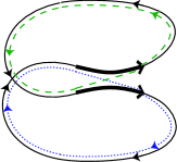
Abbildung 1: Reconnections inside a parallel 2-encounter yield a pseudo-orbit decomposing into two separate periodic orbits.

Considering orbit pairs that differ in two 2-encounters, we may thus allow for (i) both encounters being parallel, (ii) one being parallel and one antiparallel, and (iii) two antiparallel 2-encounters. Moreover, the encounters may be ordered in two different ways. In a “serial” ordering, the two stretches of each encounter follow each other immediately after an intervening loop. In an “intertwined” ordering, stretches of both encounters are traversed in alternation. Altogether, this leaves six different ways of drawing pairs of 2-encounters, as shown in Fig. 2.

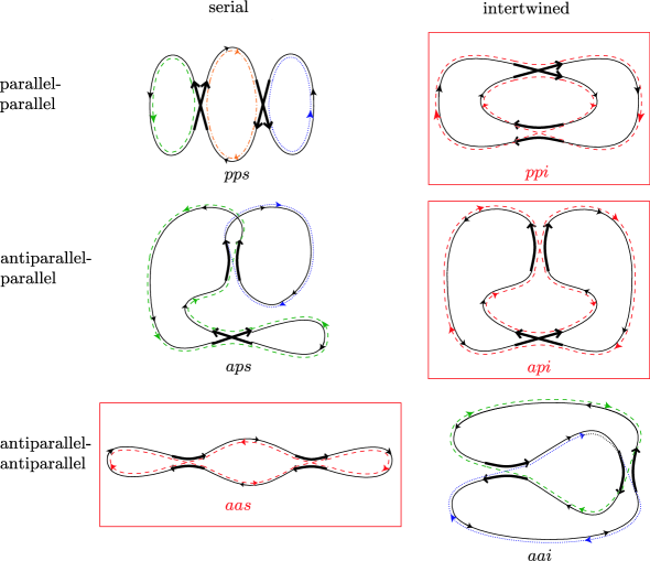
Abbildung 2: Six classes of pairs of 2-encounters, distinguished by parallel vs. antiparallel orientation of stretches, and serial vs. intertwined ordering. Reconnections inside the encounters give rise to a connected partner orbit (dashed line) only for the three cases highlighted by boxes. Otherwise the partner decomposes into several orbits, respectively depicted by dashed, dotted, and dash-dotted lines.

Reconnections inside these encounters lead either to a connected periodic orbit, or to a pseudo-orbit decomposing into several periodic orbits (depicted by dashed, dotted, and dash-dotted lines in Fig. 2). For example, two parallel encounters give rise to a connected partner only if their ordering is intertwined. If they are ordered in series, we obtain a pseudo-orbit decomposing into three disjoint orbits; this pseudo-orbit does not contribute to the form factor. One easily sees that among the six cases depicted in Fig. 2, only three (marked by boxes) lead to a connected partner orbit, namely

• two intertwined parallel encounters (abbreviated by ppi for parallel-parallel intertwined),

• pairs of one antiparallel and one parallel encounter with intertwined ordering (api), and

• two antiparallel encounters in series (aas).

Time-reversal invariant systems allow for all three kinds of encounter pairs. Apart from the partner orbits drawn in Fig. 2, we then also need to account their time-reversed versions. In contrast, for systems without time-reversal invariance only parallel encounters, and thus case ppi, need to be considered, giving rise only to the one partner orbit depicted in 2.

Incidentally, the partner orbit will always have a pair of encounters of exactly the same class as the original orbit, i.e., ppi, api, and aas, respectively. However, for api reconnections turn the antiparallel encounter into a parallel one and vice versa.

To systematically classify orbit pairs, we have to number all (at present four) encounter stretches in order of traversal by the original orbit $\gamma$, starting with one arbitrary stretch. The numbers $1,2,3,4$ are then divided into groups, one corresponding to each encounter, and we have to fix the mutual orientation of stretches inside each group. We are interested only in those divisions which give rise to a connected partner orbit; they will be referred to as “structures” of orbit pairs.

For example, in the case ppi, we will have stretches 1 and 3 forming a parallel encounter, and stretches 2 and 4 forming one further such encounter. This statement is true regardless of which stretch is chosen as the first. For instance, if we rename stretch 1 as stretch 2, we have to cyclically permute the four numbers $1\to 2\to 3\to 4\to 1$. Afterwards, we will still find one encounter of parallel stretches 1 and 3 (the former stretches 2 and 4), and one parallel encounter of stretches 2 and 4 (the former stretches 1 and 3). In this sense, all four stretches are indistinguishable. We have thus shown that ppi corresponds to one structure as defined above.

The situation becomes more complex for api. If one of the two parallel stretches is chosen as the first, we obtain a parallel encounter of stretches 1 and 3, and an antiparallel encounter of 2 and 4. However, taking one stretch of the antiparallel encounter as a reference, we obtain a parallel encounter of 2 and 4, and an antiparallel encounter of 1 and 3. Therefore, api encounters have two different structures. Both structures refer to the same orbit pairs, but differ in which of the stretches is taken as the first. The two structures may also be understood as follows: If the orbits $\gamma$ and $\gamma^{\prime}$ are cut open inside the loop preceding the “first” stretch, each structure gives rise to topologically different trajectory pairs. For api, the trajectories associated to one structure will first traverse a stretch of the parallel encounter, whereas trajectories of the second structure first traverse a stretch of the antiparallel encounter. Intuitively, the appearance of two different structures implies that api encounters are “less symmetric” than ppi encounters, since one encounter is parallel, whereas the other one involves two antiparallel stretches.

We shall see that if a family of orbit pairs is associated with several equivalent structures, all yield separate (and equal) contributions to the form factor.

Finally, for aas two among the four stretches are followed by stretches of the same encounter. If one of these two is chosen as a reference, we obtain two antiparallel encounters of stretches 1 and 2, and stretches 3 and 4, respectively. In contrast, if one of the other two stretches is considered the first, there are antiparallel encounters of stretches 1 and 4, and 2 and 3. Again, we end up with two equivalent structures.

Altogether, given time-reversal invariance, pairs of 2-encounters can have 5 different structures, one single structure related to ppi, and two structures each for api and for aas. In systems without time-reversal invariance, only parallel encounters are possible. Hence, only one among the above structures remains, the one related to (intertwined) pairs of parallel encounters.

2 Triple encounters

We now turn to pairs of orbits differing in one 3-encounter. Here, in both partner orbits, three stretches come close up to time reversal. These stretches are separated by three intervening loops, which can be arranged to form a “cloverleaf” (see Fig. 3).

We have to distinguish between two special cases. First, all three stretches may be close in phase space $\mathrel{\,\lower 0.6458pt\hbox{\begin{picture}(4.0,3.0)\put(0.0,0.3){\vector(1,0){4.0}}\put(0.0,1.5){\vector(1,0){4.0}} \put(0.0,2.7){\vector(1,0){4.0}} \end{picture}}\,}$. In this case, we speak of a “parallel cloverleaf” (pc). Obviously, pc encounters may exist even in absence of time-reversal invariance.

Partner orbits are again obtained by reshuffling intra-encounter connections. In principle, the ports can be reconnected in five different ways, depicted by $\mathrel{\,\lower 0.6458pt\hbox{\begin{picture}(4.0,3.0)\put(0.0,0.3){\vector(1,0){4.0}}\put(0.0,1.0){\vector(2,1){4.0}} \put(0.0,3.0){\vector(2,-1){4.0}} \end{picture}}\,}$ , $\mathrel{\,\lower 0.6458pt\hbox{\begin{picture}(4.0,3.0)\put(0.0,0.0){\vector(4,3){4.0}}\put(0.0,1.5){\vector(1,0){4.5}} \put(0.0,3.0){\vector(4,-3){4.0}} \end{picture}}\,}$ , $\mathrel{\,\lower 0.6458pt\hbox{\begin{picture}(4.0,3.0)\put(0.0,0.0){\vector(2,1){4.0}}\put(0.0,2.0){\vector(2,-1){4.0}} \put(0.0,2.7){\vector(1,0){4.0}} \end{picture}}\,}$ , $\mathrel{\,\lower 0.6458pt\hbox{\begin{picture}(4.0,3.0)\put(0.0,3.0){\vector(2,-1){4.0}}\put(0.0,2.0){\vector(2,-1){4.0}} \put(0.0,0.0){\vector(4,3){4.0}} \end{picture}}\,}$ , and $\mathrel{\,\lower 0.6458pt\hbox{\begin{picture}(4.0,3.0)\put(0.0,0.0){\vector(2,1){4.0}}\put(0.0,1.0){\vector(2,1){4.0}} \put(0.0,3.0){\vector(4,-3){4.0}} \end{picture}}\,}$ . However, in the first three cases only two stretches take part in the reconnection whereas the third one remains unaffected. A potential partner orbit could thus also be obtained by reconnections inside a 2-encounter. This implies that the possibilities $\mathrel{\,\lower 0.6458pt\hbox{\begin{picture}(4.0,3.0)\put(0.0,0.3){\vector(1,0){4.0}}\put(0.0,1.0){\vector(2,1){4.0}} \put(0.0,3.0){\vector(2,-1){4.0}} \end{picture}}\,}$ , $\mathrel{\,\lower 0.6458pt\hbox{\begin{picture}(4.0,3.0)\put(0.0,0.0){\vector(4,3){4.0}}\put(0.0,1.5){\vector(1,0){4.5}} \put(0.0,3.0){\vector(4,-3){4.0}} \end{picture}}\,}$ , and $\mathrel{\,\lower 0.6458pt\hbox{\begin{picture}(4.0,3.0)\put(0.0,0.0){\vector(2,1){4.0}}\put(0.0,2.0){\vector(2,-1){4.0}} \put(0.0,2.7){\vector(1,0){4.0}} \end{picture}}\,}$ have to be disregarded; the corresponding orbit pairs were already taken into account when summing over Sieber/Richter pairs in Chapter 2. In similar vein, we will always require reconnections to involve all stretches of an encounter. Among the remaining two options, $\mathrel{\,\lower 0.6458pt\hbox{\begin{picture}(4.0,3.0)\put(0.0,0.0){\vector(2,1){4.0}}\put(0.0,1.0){\vector(2,1){4.0}} \put(0.0,3.0){\vector(4,-3){4.0}} \end{picture}}\,}$ leads to a “partner” decomposing into three disjoint periodic orbits; see Fig. 3. Only reconnections according to by $\mathrel{\,\lower 0.6458pt\hbox{\begin{picture}(4.0,3.0)\put(0.0,3.0){\vector(2,-1){4.0}}\put(0.0,2.0){\vector(2,-1){4.0}} \put(0.0,0.0){\vector(4,3){4.0}} \end{picture}}\,}$  give rise to a connected partner orbit, shown in the same picture.

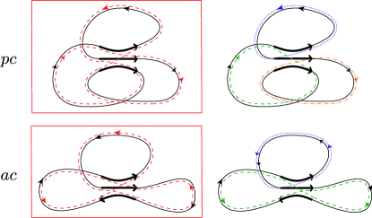
Abbildung 3: Examples for 3-encounters of type pc and ac. The reconnections on the left-hand side. give rise to a connected partner orbit (dashed lines), whereas those on the right-hand side. yield a partner decomposing into two or three periodic orbits, respectively.

One easily sees that pc encounters may have only one structure. Again numbering all encounter stretches in order of traversal, we may say that stretches 1,2, and 3 are close in phase space, irrespective of which stretch is chosen as the first.

For time-reversal invariant dynamics, there is one further way of forming 3-encounters. Instead of having three stretches close in phase space, these encounters involve only two almost parallel stretches, and a third one approximately time-reversed with respect to the initial two. In this case, we speak of an “antiparallel cloverleaf” (ac), depicted by $\mathrel{\,\lower 0.6458pt\hbox{\begin{picture}(4.0,3.0)\put(4.0,0.3){\vector(-1,0){4.0}}\put(0.0,1.5){\vector(1,0){4.0}} \put(0.0,2.7){\vector(1,0){4.0}} \end{picture}}\,}$. Since ac encounters exist only in time-reversal invariant systems, we may also read a as “anti-unitary symmetry required”.

Again, we obtain a connected partner orbit by reshuffling intra-encounter connections according to $\mathrel{\,\lower 0.6458pt\hbox{\begin{picture}(4.0,3.0)\put(0.0,3.0){\line(2,-1){4.0}}\put(0.0,2.0){\line(2,-1){4.0}} \put(0.0,0.0){\line(4,3){4.0}} \end{picture}}\,}$ ; compare Fig. 3. Here, we momentarily dropped the arrows; the encounter stretches of the partner orbit may either be close or time-reversed with respect to those of the original orbit. By reasoning analogous to pc encounters, we see that the reconnections $\mathrel{\,\lower 0.6458pt\hbox{\begin{picture}(4.0,3.0)\put(0.0,0.3){\line(1,0){4.0}}\put(0.0,1.0){\line(2,1){4.0}} \put(0.0,3.0){\line(2,-1){4.0}} \end{picture}}\,}$ , $\mathrel{\,\lower 0.6458pt\hbox{\begin{picture}(4.0,3.0)\put(0.0,0.0){\line(4,3){4.0}}\put(0.0,1.5){\line(1,0){4.5}} \put(0.0,3.0){\line(4,-3){4.0}} \end{picture}}\,}$ , and $\mathrel{\,\lower 0.6458pt\hbox{\begin{picture}(4.0,3.0)\put(0.0,0.0){\line(2,1){4.0}}\put(0.0,2.0){\line(2,-1){4.0}} \put(0.0,2.7){\line(1,0){4.0}} \end{picture}}\,}$ could equivalently be described in terms of a 2-encounter, and that $\mathrel{\,\lower 0.6458pt\hbox{\begin{picture}(4.0,3.0)\put(0.0,0.0){\line(2,1){4.0}}\put(0.0,1.0){\line(2,1){4.0}} \put(0.0,3.0){\line(4,-3){4.0}} \end{picture}}\,}$ would lead to a pseudo-orbit, this time containing two separate periodic orbits. Again, the time-reversed versions of the partners depicted in Fig. 3 also form valid partner orbits.

Orbit pairs of type ac can be described by three equivalent structures. To show this, we again number the stretches in order of traversal by $\gamma$, starting from an arbitrary one. If that reference stretch is the one approximately time-reversed with respect to the others, we have stretch 1 antiparallel to 2 and 3, which are mutually close. Choosing a different reference, we are led to two further structures, with 2 antiparallel to 1 and 3, and 3 antiparallel to 1 and 2. Again, if the orbits $\gamma$ and $\gamma^{\prime}$ are cut open in the loop preceding the first stretch, each structure gives rise to topologically different trajectory pairs.

To summarize, systems without time-reversal invariance allow for one “cloverleaf” structure, related to pc, whereas in presence of time-reversal invariance we observe 4 such structures, including 3 stemming from ac encounters.

3 Symbolic dynamics

Given symbolic dynamics, the orbit pairs introduced in the preceding Sections can be characterized through their symbols sequences. Within each encounter, stretches are either very close in phase space and thus labelled by the same symbol sequence ${\cal E}_{\alpha}$, or almost mutually time-reversed and thus denoted by mutually time-reversed sequences ${\cal E}_{\alpha}$ and $\bar{{\cal E}}_{\alpha}$. Each of the intervening loops comes with its own symbol sequence, to be denoted by ${\cal A},{\cal B},\ldots$. The symbol strings of the orbits $\gamma$ and $\gamma^{\prime}$ are built as alternating series of encounter and loop sequences. If a given loop ${\cal A}$ of $\gamma$ connects, say, stretches with symbol sequences ${\cal E}_{1}$ and ${\cal E}_{2}$, the corresponding loop of $\gamma^{\prime}$ must either connect stretches with the same sequences, as in $\ldots{\cal E}_{1}{\cal A}{\cal E}_{2}\ldots$, or appear in time-reversed form, like $\ldots\bar{{\cal E}}_{2}\bar{{\cal A}}\bar{{\cal E}}_{1}\ldots$.

For instance, two intertwined parallel 2-encounters ${\cal E}_{1}\ldots{\cal E}_{1}$ and ${\cal E}_{2}\ldots{\cal E}_{2}$ entail the symbol sequence $\gamma={\cal E}_{1}{\cal A}{\cal E}_{2}{\cal B}{\cal E}_{1}{\cal C}{\cal E}_{2}{\cal D}$. Reconnections yield a partner with the symbol sequence $\gamma^{\prime}={\cal E}_{1}{\cal A}{\cal E}_{2}{\cal D}{\cal E}_{1}{\cal C}{\cal E}_{2}{\cal B}$. Likewise, intertwined parallel and antiparallel 2-encounters ${\cal E}_{1}\ldots{\cal E}_{1}$ and ${\cal E}_{2}\ldots\bar{{\cal E}}_{2}$ lead to $\gamma={\cal E}_{1}{\cal A}{\cal E}_{2}{\cal B}{\cal E}_{1}{\cal C}\bar{{\cal E}}_{2}{\cal D}$ and a partner orbit $\gamma^{\prime}={\cal E}_{1}{\cal A}{\cal E}_{2}\bar{{\cal C}}\bar{{\cal E}}_{1}\bar{{\cal D}}{\cal E}_{2}{\cal B}$ with loops ${\cal C}$ and ${\cal D}$ reversed in time. Two serial antiparallel encounters ${\cal E}_{1}\ldots\bar{{\cal E}}_{1}$ and ${\cal E}_{2}\ldots\bar{{\cal E}}_{2}$ can be combined into the sequences $\gamma={\cal E}_{1}{\cal A}\bar{{\cal E}}_{1}{\cal B}{\cal E}_{2}{\cal C}\bar{{\cal E}}_{2}{\cal D}$ and $\gamma^{\prime}={\cal E}_{1}{\cal A}\bar{{\cal E}}_{1}\bar{{\cal D}}{\cal E}_{2}{\cal C}\bar{{\cal E}}_{2}\bar{{\cal B}}$.

Parallel 3-encounters ${\cal E}\ldots{\cal E}\ldots{\cal E}$ lead to orbit pairs $\gamma={\cal E}{\cal A}{\cal E}{\cal B}{\cal E}{\cal C}$, $\gamma^{\prime}={\cal E}{\cal A}{\cal E}{\cal C}{\cal E}{\cal B}$, whereas ${\cal E}\ldots{\cal E}\ldots\bar{{\cal E}}$ denotes an encounter with the third stretch antiparallel to the first two. In the latter case, orbit pairs have symbol sequences of the form $\gamma={\cal E}{\cal A}{\cal E}{\cal B}\bar{{\cal E}}{\cal C}$, $\gamma^{\prime}={\cal E}{\cal A}{\cal E}\bar{{\cal B}}\bar{{\cal E}}\bar{{\cal C}}$.

4 Orbit pairs responsible for all orders in $\tau$

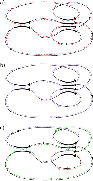
Abbildung 4: a) Solid line: Periodic orbit $\gamma$ with one 4-encounter and one 2-encounter highlighted by bold arrows. Dashed line: Partner $\gamma^{\prime}$ differing from $\gamma$ by connections in these encounters. b) Dotted line: One further orbit, differing from $\gamma$ in the same set of encounters. c) Other reconnections yield a pseudo-orbit decomposing into three periodic orbits (dashed, dotted, and dash-dotted).

To obtain all orders of the power series of $K(\tau)$, we have to account for orbit pairs differing in any number of $l$-encounters, with arbitrary $l\geq 2$.

Let us first sketch two more examples. Fig. 4a highlights two encounters inside a periodic orbit, one 2-encounter and one 4-encounter. The stretches involved can be reconnected in several different ways. Some of these reconnections, like in Fig. 4a or b, yield connected partner orbits. Other reconnections, as in Fig. 4c, give rise to a pseudo-orbit decomposing into a number of disjoint periodic orbits, and thus do not contribute to the form factor. Since both encounters involve only parallel stretches, orbit pairs as in Fig. 4a and b exist both in systems with and without time-reversal invariance.

For time-reversal invariant dynamics, we also must allow for encounters whose stretches get close only up to time reversal. Correspondingly, loops inside mutual partner orbits may be related by time reversal. See Fig. 5a for an example of two orbits differing in encounters $\mathrel{\,\lower 0.6458pt\hbox{\begin{picture}(4.0,3.0)\put(4.0,0.8){\vector(-1,0){4.0}}\put(0.0,2.0){\vector(1,0){4.0}} \end{picture}}\,}$ and $\mathrel{\,\lower 0.6458pt\hbox{\begin{picture}(4.0,3.0)\put(4.0,0.3){\vector(-1,0){4.0}}\put(0.0,1.5){\vector(1,0){4.0}} \put(0.0,2.7){\vector(1,0){4.0}} \end{picture}}\,}$. The pseudo-orbit obtained in Fig. 5b does not contribute to the form factor.

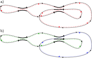
Abbildung 5: a) Periodic orbit $\gamma$ with one 2- and one 3-encounter highlighted, and a partner $\gamma^{\prime}$ obtained by reconnection; the encounters depicted exist only in time-reversal invariant systems. b) Again, different reconnections lead to a ”pseudo-orbit”, this time decomposing into two separate periodic orbits (dashed and dotted).

We thus obtain a natural extension of Berry’s diagonal approximation. Instead of considering only pairs of orbits which exactly coincide (or are mutually time-reversed), we employ all pairs whose members are composed of similar (up to time reversal) loops.

We have to classify these orbit pairs. The two orbits of each pair differ in a number $v_{l}$ of $l$-encounters; we shall assemble these numbers to a “vector” $\vec{v}=(v_{2},v_{3},\ldots)$. The total number of encounters is given by $V(\vec{v})=\sum_{l\geq 2}v_{l}$. The number of orbit stretches involved in encounters, coinciding with the number of intervening loops, reads $L(\vec{v})=\sum_{l\geq 2}lv_{l}$.

As we have seen for orbit pairs differing in two 2-encounters or in one 3-encounter, orbit pairs related to the same $\vec{v}$ may have different structures. In general, structures are defined as follows: Starting from an arbitrarily chosen reference stretch, the $L(\vec{v})$ encounter stretches are numbered in order of traversal by $\gamma$. Each structure now corresponds to one way of

1. assembling the $L(\vec{v})$ labels into groups, each corresponding to one encounter,

2. fixing the mutual orientation of stretches in each group, like $\mathrel{\,\lower 0.6458pt\hbox{\begin{picture}(4.0,3.0)\put(0.0,0.8){\vector(1,0){4.0}}\put(0.0,2.0){\vector(1,0){4.0}} \end{picture}}\,}$ vs. $\mathrel{\,\lower 0.6458pt\hbox{\begin{picture}(4.0,3.0)\put(4.0,0.8){\vector(-1,0){4.0}}\put(0.0,2.0){\vector(1,0){4.0}} \end{picture}}\,}$, or $\mathrel{\,\lower 0.6458pt\hbox{\begin{picture}(4.0,3.0)\put(0.0,0.3){\vector(1,0){4.0}}\put(0.0,1.5){\vector(1,0){4.0}} \put(0.0,2.7){\vector(1,0){4.0}} \end{picture}}\,}$ vs. $\mathrel{\,\lower 0.6458pt\hbox{\begin{picture}(4.0,3.0)\put(4.0,0.3){\vector(-1,0){4.0}}\put(0.0,1.5){\vector(1,0){4.0}} \put(0.0,2.7){\vector(1,0){4.0}} \end{picture}}\,}$ (if the system is time-reversal invariant), and

3. reconnecting the stretches to form a non-decomposing partner orbit.

The third point is particularly important if several reconnections in the same set of encounters lead to different connected partner orbits, as in Figs. 4a and b. In this case, each such reconnection gives rise to an orbit pair of a different structure. We did not meet this situation in the examples of Subsections 1-3. (Note that for time-reversal invariant systems, orbit pairs $(\gamma,\gamma^{\prime})$ and $(\gamma,{\cal T}\gamma^{\prime})$ distinguished only by time-reversal of the partner orbit are considered as belonging to the same structure.)

Again, some orbit pairs can be described in terms of several equivalent structures, depending on which stretch is taken as the first. If we, however, imagine the orbits $\gamma,\gamma^{\prime}$ cut open in the loop preceding the first stretch, each structure gives rise to a topologically different class of trajectory pairs. Another alternative definition of structures uses (numbered) loops rather than encounter stretches: Each structure corresponds to a different ordering – and, given time-reversal invariance, different sense of traversal – of the loops of $\gamma$ inside the partner orbit $\gamma^{\prime}$.

To evaluate the spectral form factor, we need to determine the number $N(\vec{v})$ of structures related to the same $\vec{v}$.

Apart from vectors $\vec{v}$ and structures, orbit pairs can be characterized by the phase-space separations between encounter stretches. In Chapter 2, we introduced stable and unstable coordinates $s,u$ measuring the separation between stretches of a 2-encounter. We have to define similar coordinates for arbitrary $l$-encounters, and derive a density $w_{T}(s,u)$ of phase-space separations analogous to (18). The double sum (25) over orbits defining the spectral form factor will then be written as a sum of contributions from families of orbit pairs, with a weight proportional to $N(\vec{v})w_{T}(s,u)$.

In the following Chapter, we will study the phase-space geometry of encounters and determine the density $w_{T}(s,u)$. The purely combinatorial task of determining the number of structures $N(\vec{v})$ for arbitrary $\vec{v}$ is attacked in Chapter 5 with the help of permutation theory. We will then obtain expansions of $K(\tau)$ for individual chaotic systems, in line with the respective predictions of the GUE and the GOE.

5 Summary

We define $l$-encounters as regions inside an orbit $\gamma$ where $l$ orbit stretches are mutually close up to time reversal. We consider orbit pairs differing by reconnections inside an arbitrary number $v_{l}$ of $l$-encounters; both partners must be connected periodic orbits. The orbit pairs are further classified by “structures” (i.e., ordering and mutual orientation of stretches, and reconnections) and phase-space separations. The $\tau^{3}$-contribution originates from orbit pairs differing in two 2-encounters (1 structure for systems without ${\cal T}$ invariance, altogether 5 structures in presence ${\cal T}$ invariance) or in one 3-encounter (1 structure without ${\cal T}$ invariance, 4 structures with ${\cal T}$ invariance).

Kapitel 4 Phase-space geometry of encounters

In the present Chapter, we want to determine the contribution to the form factor originating from all orbit pairs of a given structure. To that end, we have to extend the results of Chapter 2, and describe the phase-space geometry of encounters with arbitrary number of stretches $l$.

1 Encounters

We first need to introduce suitable stable and unstable coordinates. To do so, we again consider a Poincaré surface of section ${\cal P}$ orthogonal to the orbit at an arbitrary phase-space point ${\bf x}_{1}$ (passed at time $t_{1}$) inside one of the encounter stretches. The remaining stretches pierce through ${\cal P}$ at times $t_{j}$ ($j=2,\ldots,l$) in points ${\bf x}_{j}$. If the $j$-th encounter stretch is close to the first one in phase space, we must have ${\bf x}_{j}\approx{\bf x}_{1}$; if it is almost time-reversed with respect to the first one, we have ${\cal T}{\bf x}_{j}\approx{\bf x}_{1}$. In the following, we shall use the shorthand ${\bf y}_{j}\approx{\bf x}_{1}$ with ${\bf y}_{j}$ either ${\bf x}_{j}$ or ${\cal T}{\bf x}_{j}$.

The small displacement ${\bf y}_{j}-{\bf x}_{1}$ can be decomposed into components along the stable and unstable directions at ${\bf x}_{1}$,

$${\bf y}_{j}-{\bf x}_{1}=\hat{s}_{j}{\bf e}^{s}({\bf x}_{1})+\hat{u}_{j}{\bf e}^{u}({\bf x}_{1})\,.$$ (1)

Thus, each encounter is described by $l-1$ pairs of stable coordinates $\hat{s}_{j}$ and unstable coordinates $\hat{u}_{j}$. These coordinates depend on the location of ${\cal P}$; as $t_{1}$ grows, stable coordinates asymptotically decrease and unstable coordinates asymptotically increase. We will later subject $\hat{s}_{j}$, $\hat{u}_{j}$ to a coordinate transformation yielding new coordinates to be denoted by $s_{j}$, $u_{j}$; hence the “hats” in (1).

By definition, an $l$-encounter lasts as long as all $l$ stretches are mutually close. We thus have to demand the stable and unstable differences $|\hat{s}_{j}|$, $|\hat{u}_{j}|$ of all stretches from the first one to be smaller than our constant $c$. As a consequence, the mutual difference between two stretches different from the first one is limited by $2c$. “Fringes” where only a few stretches remain close are not regarded as part of the encounter.

We can now generalize the formula (4) for the duration $t_{\rm enc}$ of an encounter. Each of the unstable coordinates $|\hat{u}_{j}|$ needs the time $\frac{1}{\lambda}\ln\frac{c}{|\hat{u}_{j}|}$ to reach $c$. The encounter ends as soon as the first of these components passes the threshold, i.e., after a time

$$t_{u}\sim\min_{j}\left\{\frac{1}{\lambda}\ln\frac{c}{|\hat{u}_{j}|}\right\}\,.$$ (2)

Similarly, the time since the beginning of the encounter (i.e., since the last of the stable coordinates has fallen below $c$) can be estimated as

$$t_{s}\sim\min_{j}\left\{\frac{1}{\lambda}\ln\frac{c}{|\hat{s}_{j}|}\right\}\,.$$ (3)

As for 2-encounters, we will refer to $t_{u}$ and $t_{s}$ as the durations of the “head” and the “tail” of the encounter. Both quantities sum up to the overall duration of the encounter

$$t_{\rm enc}=t_{s}+t_{u}\sim\frac{1}{\lambda}\ln\frac{c^{2}}{\max_{i}\{|\hat{s}_{i}|\}\max_{j}\{|\hat{u}_{j}|\}}\,;$$ (4)

in view of Eq. (1), $t_{\rm enc}$ remains invariant if the Poincaré section ${\cal P}$ is shifted through the encounter.

An $l$-encounter involves $l$ different orbit stretches whose initial and final phase-space points will be referred to as “entrance” and “exit ports”. If all encounter stretches are (almost) parallel, as in $\mathrel{\,\lower 0.6458pt\hbox{\begin{picture}(4.0,3.0)\put(0.0,0.3){\vector(1,0){4.0}}\put(0.0,1.5){\vector(1,0){4.0}} \put(0.0,2.7){\vector(1,0){4.0}} \end{picture}}\,}$, all entrance ports are located on the same side of the encounter, and the exit ports are located on the opposite side. If the encounter involves mutually time-reversed orbit stretches like $\mathrel{\,\lower 0.6458pt\hbox{\begin{picture}(4.0,3.0)\put(4.0,0.3){\vector(-1,0){4.0}}\put(0.0,1.5){\vector(1,0){4.0}} \put(0.0,2.7){\vector(1,0){4.0}} \end{picture}}\,}$, this is no longer the case. Thus, it is useful to introduce the following convention: All ports on the side where the (arbitrarily chosen) first stretch begins are called “left ports”, while those on the opposite side are “right ports”. For parallel encounters, “entrance” and “left” are synonymous, as well as “exit” and “right”.

2 Partner orbits

The partner orbits $(\gamma,\gamma^{\prime})$ differ from one another only inside the encounters, by their connections between left and right ports. We shall number these ports in order of traversal by $\gamma$, such that the $j$-th encounter stretch of $\gamma$ connects left port $j$ to right port $j$. Inside $\gamma^{\prime}$, the left port $j$ is connected to a different right port $k$; see Figs. 1a and b for possible reconnections in a 3- and a 6-encounter.

When reshuffling connections, we must mix all stretches of a given encounter. In contrast, Fig. 1c shows reconnections only between stretches 1 and 2, 3 and 4, and stretches 5 and 6 of a 6-encounter which therefore decomposes into three separate 2-encounters.

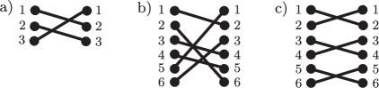
Abbildung 1: Possible connections between left and right ports in partner orbits $\gamma^{\prime}$. In c), the encounter splits into three pieces respectively containing the two upper, middle, and lower stretches.

1 Piercing points

Abbildung 2: Piercing points of orbits $\gamma$,$\gamma^{\prime}$ differing in a 3-encounter; inside $\gamma^{\prime}$, the left ports 1, 2, 3 are connected to the right ports 2, 3, 1, respectively. a) Sketch in configuration space. b) Stable and unstable coordinates in a Poincaré section ${\cal P}$.

The partner $\gamma^{\prime}$ also pierces through our Poincaré section ${\cal P}$. The piercing point of the stretch connecting left port $j$ to right port $k$ will be denoted by ${\bf x}_{j}^{\prime}$. Similarly as for the piercings of $\gamma$, the shorthand ${\bf y}_{j}^{\prime}$ will represent either ${\bf x}_{j}^{\prime}$ or ${\cal T}{\bf x}_{j}^{\prime}$, depending on whether the stretch in question is parallel or antiparallel with respect to the first one. See Fig. 2a for the example of a 3-encounter $\mathrel{\,\lower 0.6458pt\hbox{\begin{picture}(4.0,3.0)\put(4.0,0.3){\vector(-1,0){4.0}}\put(0.0,1.5){\vector(1,0){4.0}} \put(0.0,2.7){\vector(1,0){4.0}} \end{picture}}\,}$.

Like in case of 2-encounters the piercing points of $\gamma^{\prime}$ are determined by those of $\gamma$. In particular, the unstable coordinates of a point ${\bf y}_{j}^{\prime}$ always depend on the following right port. If two stretches of $\gamma$ and $\gamma^{\prime}$ lead to the same right port, they have to approach each other at least for the duration of the encounter head; for the relevant encounters this duration is of the order $T_{E}\to\infty$. Since the phase-space difference shrinks in time, it may have only a very small unstable component, meaning that the unstable coordinates of ${\bf y}_{j}$ and ${\bf y}_{j}^{\prime}$ practically coincide. Likewise, the stable coordinate of ${\bf y}_{j}^{\prime}$ is determined by the previous left port, since stretches with the same left port approach for large negative times. If a stretch of $\gamma^{\prime}$ connects left port $j$ to right port $k$, it thus pierces through our Poincaré section with stable and unstable coordinates approximately given by

$$\hat{s}_{j}^{\prime}=\hat{s}_{j},\ \ \ \ \hat{u}_{j}^{\prime}=\hat{u}_{k}\,;$$ (5)

this generalizes the relation (5) for 2-encounters.

For the 3-encounter of Fig. 2a, the partner orbit $\gamma^{\prime}$ has left ports 1, 2, and 3 of $\gamma$ respectively connected to the right ports 2, 3, and 1. The first stretch of $\gamma^{\prime}$ connects left port 1 to right port 2 and pierces through ${\cal P}$ in ${\bf y}_{1}^{\prime}$ with $\hat{s}_{1}^{\prime}=\hat{s}_{1}=0$, $\hat{u}_{1}^{\prime}=\hat{u}_{2}$. The second stretch pierces through ${\cal P}$ in ${\bf y}_{2}^{\prime}$ with $\hat{s}_{2}^{\prime}=\hat{s}_{2}$, $\hat{u}_{2}^{\prime}=\hat{u}_{3}$, and the third one in ${\bf y}_{3}^{\prime}$ with $\hat{s}_{3}^{\prime}=\hat{s}_{3}$, $\hat{u}_{3}^{\prime}=\hat{u}_{1}=0$; see Fig. 2b.

2 Action difference

We have already seen that for $\gamma$, $\gamma^{\prime}$ differing in one 2-encounter, the action difference is given by the product of the stable and unstable separations between the two encounter stretches. In order to generalize to $\gamma$, $\gamma^{\prime}$ differing in an $l$-encounter, we can imagine the partner orbit $\gamma^{\prime}$ constructed out of $\gamma$ by $l-1$ successive steps. For a 3-encounter $\mathrel{\,\lower 0.6458pt\hbox{\begin{picture}(4.0,3.0)\put(0.0,0.3){\line(1,0){4.0}}\put(0.0,1.5){\line(1,0){4.0}} \put(0.0,2.7){\line(1,0){4.0}} \end{picture}}\,}$, we may first reconnect the two upper stretches as in $\mathrel{\,\lower 0.6458pt\hbox{\begin{picture}(4.0,3.0)\put(0.0,0.3){\line(1,0){4.0}}\put(0.0,1.0){\line(2,1){4.0}} \put(0.0,3.0){\line(2,-1){4.0}} \end{picture}}\,}$, and then the stretches starting from the second and third left port as in $\mathrel{\,\lower 0.6458pt\hbox{\begin{picture}(4.0,3.0)\put(0.0,3.0){\line(2,-1){4.0}}\put(0.0,2.0){\line(2,-1){4.0}} \put(0.0,0.0){\line(4,3){4.0}} \end{picture}}\,}$. One further example, involving a 4-encounter, is given in Fig. 3. Each step interchanges the right ports of two encounter stretches and contributes to the action difference an amount given by the product of their stable and unstable separations. At the same time, the two piercing points change their position as discussed in Subsection 2.

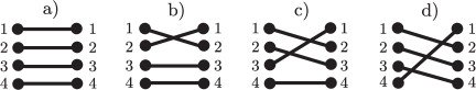
Abbildung 3: Steps from connections in $\gamma$ (depicted in a) to those in $\gamma^{\prime}$ (shown in d), in each step interchanging right ports of two encounter stretches.

This step-by-step process suggests a useful transformation of coordinates. Let $s_{j}$, $u_{j}$ denote the stable and unstable differences between the two stretches affected by the $j$-th step. Note that in contrast to $\hat{s}_{j}$, $\hat{u}_{j}$ the index $j$ no longer represents encounter stretches $2,\ldots,l$ but steps $1,\ldots,(l-1)$. Now, the change of action in each step is simply given by $s_{j}u_{j}$. Summing over all steps, we obtain a total action difference

$$\Delta S=\sum_{j=1}^{l-1}s_{j}u_{j}\,.$$ (6)

The transformation leading from $\hat{s}_{j}$, $\hat{u}_{j}$ to $s_{j}$, $u_{j}$ is linear and volume-preserving. To explicitly express $s_{j}$, $u_{j}$ as a function of $\hat{s}_{j}$ and $\hat{u}_{j}$, we first consider reconnections as given above for $l=3$, or depicted in Fig. 3d for $l=4$. We proceed from Fig. 3a to 3d in $l-1=3$ steps. In the $j$-th step, we change connections between left ports $j$ and $j+1$, and right ports 1 and $j+1$. Recall that stable and unstable coordinates of piercing points are determined by the left and right ports, respectively. Thus, the separation between the stretches affected has a stable component $s_{j}=\hat{s}_{j+1}-\hat{s}_{j}$ and an unstable component $u_{j}=\hat{u}_{j+1}-\hat{u}_{1}=\hat{u}_{j+1}$. The Jacobian of the transformation $\hat{s},\hat{u}\to s,u$ is equal to 1. All other permissible reconnections can be brought to a form similar to Fig. 3d, albeit with different $l$, by appropriately changing the numbering of stretches; hence they allow for the same step-by-step procedure. (An interpretation of this procedure in the context of permutations will be given in Subsection 1.)

Due to the elegant form of Eq. (6), it will be convenient to use $s_{j}$, $u_{j}$ rather than $\hat{s}_{j}$, $\hat{u}_{j}$ in defining the encounter regions, demanding all $|s_{j}|$, $|u_{j}|$ to be smaller than our bound $c$; the encounter duration (4) is changed accordingly.

Employing Eq. (1), one easily shows that $\Delta S$ remains invariant if the Poincaré section ${\cal P}$ is shifted through the encounter. Moreover, if the orbits $\gamma$ and $\gamma^{\prime}$ differ in several encounters (labeled by $\alpha=1,\ldots,V$), the total action difference is additive in their contributions, and each is given by Eq. (6); i.e., we have

$$\Delta S=\sum_{\alpha,j}s_{\alpha j}u_{\alpha j}\,.$$ (7)

Like in case of Sieber/Richter pairs, the relevant orbit pairs with $\Delta S\sim\hbar$ have stable and unstable coordinates of the order $\sqrt{\hbar}$, and hence encounter durations (4) of the order of the Ehrenfest time.

Finally, the relative difference between the stability amplitudes of the relevant partner orbits $\gamma$, $\gamma^{\prime}$ can be neglected in the semiclassical limit. The arguments used in Subsection 3 immediately carry over, given that the two partner orbits $\gamma$, $\gamma^{\prime}$ are close everywhere up to time reversal.

3 Necessity of non-vanishing loops

Contributions to the form factor arise only from sets of encounters whose stretches are separated by non-vanishing loops, i.e., do not overlap. After all, we obtained partner orbits by reshuffling connections between ports, where the orbit either enters an encounter stretch coming from an intervening loop, or leaves the encounter to follow an intervening loop. This procedure requires separated encounter stretches.

Like for Sieber/Richter pairs, we need to check whether our method of “generating” partner orbits can be extended to encounters with overlapping stretches, i.e., whether with the above prescription we miss any orbit pairs related to encounters. This question is investigated in detail in Appendix 11, showing that no such orbit pairs are missed, and that overlapping stretches indeed do not contribute to the form factor. Here we just want to list the main ideas.

First, assume that two stretches of different encounters overlap. In this case, the two encounters effectively merge, leaving one larger encounter with more internal stretches, see Fig. 4. The partners are thus seen as differing in one larger encounter (e.g., a 3-encounter), rather than in two smaller ones (e.g., two overlapping 2-encounters).

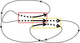
Abbildung 4: Two 2-encounters (marked by boxes) overlap in one stretch and thus merge to a 3-encounter (solid bold arrows)

As in Subsection 4, overlapping antiparallel stretches have to be regarded as one single stretch reflected at a hard wall. There is no way to reconnect such stretches to form a partner orbit.

Finally, we shall see that parallel stretches can overlap (or come very close in time) only if they follow multiple revolutions of a shorter orbit $\tilde{\gamma}$. In this case, several different encounters may lead to the same partner orbit. We will show in Appendix 11.C how to select one of these encounters. The resulting condition will be slightly more complicated than just leaving out encounters with overlapping stretches but in the semiclassical limit leads to the same contributions to the form factor.

4 Statistics of encounter sets

The statistics of close self-encounters inside periodic orbits can now be established using the same two ingredients as in the case of 2-encounters: the ergodicity of the classical motion, and the requirement of non-vanishing loops.

We will consider sets of encounters within orbit pairs $(\gamma,\gamma^{\prime})$ with fixed $\vec{v}$ and fixed structure. Each of the $V$ encounters of $\gamma$ is parametrized with the help of a Poincaré section ${\cal P}_{\alpha}$ ($\alpha=1,\ldots,V$) crossing the orbit at an arbitrary phase-space point inside the encounter, traversed at time $t_{\alpha 1}$. The orbit again pierces through these sections at times $t_{\alpha j}$ with $j=2,\ldots,l_{\alpha}$ numbering the remaining stretches of the $\alpha$-th encounter. The first piercing may occur anywhere inside the orbit at a time $0<t_{11}<T$, $T$ denoting the period. The remaining $t_{\alpha j}$ follow in an order fixed by the structure at times $t_{11}<t_{\alpha j}<T+t_{11}$. Each of the $v_{l}$ $l$-encounters is characterized by $l-1$ pairs of stable and unstable coordinates $s_{\alpha j}$, $u_{\alpha j}$ ($j=1,\ldots,l-1$), which in total make for $2\sum_{l\geq 2}(l-1)v_{l}=2(L-V)$ components.

We proceed to derive a density $w_{T}(s,u)$ of phase-space separations $s$, $u$. To understand the normalization of $w_{T}(s,u)$, recall that the separations $s$ and $u$ depend on the location of the Poincaré sections ${\cal P}_{\alpha}$. If ${\cal P}_{\alpha}$ is shifted through the corresponding encounter, the stable and unstable coordinates change while the contributions to the action difference $\Delta S_{\alpha j}=s_{\alpha j}u_{\alpha j}$ remain invariant. To make sure that each encounter is counted exactly one, we demand that the integral $\int d^{L-V}s\,d^{L-V}u\,w_{T}(s,u)\prod_{\alpha j}\delta(\Delta S_{\alpha j}-s_{\alpha j}u_{\alpha j})$ yields the density of encounter sets in an orbit $\gamma$ leading to orbit pairs $(\gamma,\gamma^{\prime})$ with given structure and action difference components $\Delta S_{\alpha j}$. We have to understand $w_{T}(s,u)$ as averaged over the ensemble of all periodic orbits $\gamma$ with period $T$ in a given time window, weighted with $|A_{\gamma}|^{2}$. Again, such averaging allows us to invoke ergodicity even for periodic orbits. (A more careful implementation will be given in Appendix 10.A.)

To determine $w_{T}(s,u)$, we need to count piercings through the Poincaré sections ${\cal P}_{\alpha}$. We first assume that all times $t_{\alpha 1}$ and thus all sections ${\cal P}_{\alpha}$ are fixed. Ergodicity then implies that for each section, the probability of a further piercing occurring in a time interval $(t_{\alpha j},t_{\alpha j}+dt_{\alpha j})$ with stable and unstable coordinates inside $(\hat{s}_{\alpha j},\hat{s}_{\alpha j}+d\hat{s}_{\alpha j})\times(\hat{u}_{\alpha j},\hat{u}_{\alpha j}+d\hat{u}_{\alpha j})$ is given by $\frac{1}{\Omega}d\hat{s}_{\alpha j}d\hat{u}_{\alpha j}dt_{\alpha j}$. This probability holds for all $l_{\alpha}-1$ additional piercings ($j=2,\ldots,l_{\alpha}$) through each of the $V$ sections. Since the transformation leading from $\hat{s}$, $\hat{u}$ to $s$, $u$ is volume-preserving, the same uniform probability applies to the components $s_{\alpha j}$, $u_{\alpha j}$. We can therefore determine the number $\rho_{T}(s,u)\,d^{L-V}s\,d^{L-V}u\,d^{L-V}t$ of sets of $L-V$ piercings through our sections ${\cal P}_{\alpha}$ occurring in time intervals $(t_{\alpha j},t_{\alpha j}+dt_{\alpha j})$, $j=2,\ldots,l_{\alpha}$, with stable and unstable coordinates inside $(s_{\alpha j},s_{\alpha j}+ds_{\alpha j})$, $(u_{\alpha j},u_{\alpha j}+du_{\alpha j})$, $j=1,\ldots,l_{\alpha}-1$; we may expect $\rho_{T}(s,u)$ equal to $1/\Omega^{L-V}$.

However, recall that we are only interested in encounters separated by non-vanishing loops. To implement that restriction, we employ a suitable characteristic function $\Theta_{T}(s,u,t)$ which vanishes if the piercings described by $s$, $u$ and $t$ correspond to overlapping stretches, and otherwise equals $1$. We thus obtain

$$\rho_{T}(s,u,t)=\Theta_{T}(s,u,t)\frac{1}{\Omega^{L-V}}\,.$$ (8)

Proceeding towards $w_{T}(s,u)$ we integrate over the $L-V$ piercing times $t_{\alpha j}$, $j\geq 2$, still for fixed Poincaré sections ${\cal P}_{\alpha}$. The integral yields a density for sets of $L-V$ piercings, characterized only by their stable and unstable coordinates $s$, $u$.

To finally get to $w_{T}$, we must keep track of all encounters along the orbits in question. To that end we have to consider all possible positions of Poincaré sections and hence integrate over the $V$ times $t_{\alpha 1}$ (of the reference piercings) as well. Doing so, we count each encounter for a time $t_{\rm enc}^{\alpha}$, since we may move each Poincaré section to any position inside the duration of the encounter. Each set of encounters is thus weighted with the product of all durations $\prod_{\alpha}t_{\rm enc}^{\alpha}$. In order to count each encounter set exactly once, we divide out the factor $\prod_{\alpha}t_{\rm enc}^{\alpha}$, and arrive at the desired density

$$w_{T}(s,u)=\frac{\int d^{L}t\,\Theta_{T}(s,u,t)}{\Omega^{L-V}\prod_{\alpha}t_{\rm enc}^{\alpha}}\,.$$ (9)

Again, loops shorter than the classical relaxation time $t_{\rm cl}$ will entail small corrections to the uniform piercing probability and therefore to (9); in the semiclassical limit these corrections are negligible due to $t_{\rm cl}\ll T_{E},T_{H}$.

It remains to evaluate the $L$-fold time integral in Eq. (9). The integration over $t_{11}$ runs from 0 to $T$; it will be done as the last integral and then give a factor $T$. The $L-1$ other $t_{\alpha j}$ must lie inside the interval $(t_{11},t_{11}+T)$ and respect the ordering dictated by the structure in question.

Moreover, we only consider encounter stretches separated by intervening loops. As a consequence, the piercing times $t_{\alpha j}$ of subsequent stretches need to respect certain minimal (time) distances. Let us first assume that all encounters are parallel such that the orbit passes through each stretch from tail to head. In this case, the time between the piercings of two subsequent stretches must be so large as to contain both the head of the first stretch and, after a non-vanishing loop, the tail of the second stretch. For time-reversal invariant systems, encounter stretches may also be time-reversed compared to the first stretch of the respective encounter; in this case head and tail of the corresponding stretch switch their roles. If we sum up all minimal distances between subsequent piercings, each stretch will appear in that sum once with head and tail, and thus give a contribution $t_{\rm enc}^{\alpha}=t_{s}^{\alpha}+t_{u}^{\alpha}$. Altogether, the minimal distances sum up to the total duration of all encounter stretches $\sum_{\alpha}l_{\alpha}t_{\rm enc}^{\alpha}$, regardless of the structure considered.

The minimal distances effectively reduce the integration range, as we may proceed to a new set of times $\tilde{t}_{\alpha j}$ obtained by subtracting from $t_{\alpha j}$ both $t_{11}$ and the sum of minimal distances between $t_{11}$ and $t_{\alpha j}$. The $\tilde{t}_{\alpha j}$ just have to obey the same ordering as the times $t_{\alpha j}$, and lie in an interval $(0,T-\sum_{\alpha}l_{\alpha}t_{\rm enc}^{\alpha})$, where the subtrahend is the total sum of minimal distances. If we choose to label the $L-1$ times $\tilde{t}_{\alpha j}$ not by $\alpha$ and $j$, but in order of traversal (indexed by one subscript $m=1,2,\ldots,L-1$), the integration range may simply be written as $0<\tilde{t}_{1}<\tilde{t}_{2}<\ldots<\tilde{t}_{L-1}<T-\sum_{\alpha}l_{\alpha}t_{\rm enc}^{\alpha}$. We are therefore left with a trivial $(L-1)$-fold integral over unity, yielding the density

$$w_{T}(s,u) = \frac{T}{\Omega^{L-V}\prod_{\alpha}t_{\rm enc}^{\alpha}}\int_{0}^{T-\sum_{\alpha}l_{\alpha}t_{\rm enc}^{\alpha}}d\tilde{t}_{L-1}\int_{0}^{\tilde{t}_{L-1}}d\tilde{t}_{L-2}\ldots\int_{0}^{\tilde{t}_{2}}d\tilde{t}_{1}$$ (10)

$$= \frac{T(T-\sum_{\alpha}l_{\alpha}t_{\rm enc}^{\alpha})^{L-1}}{(L-1)!\;\Omega^{L-V}\prod_{\alpha}t_{\rm enc}^{\alpha}}\,.$$

Crucially, $w_{T}(s,u)$ depends only on $\vec{v}$ but not on the structure considered, and that fact strongly simplifies our treatment.

We can now determine the (average) number $P_{T}^{\vec{v}}(\Delta S)d\Delta S$ of partners differing from $\gamma$ in $v_{l}$ $l$-encounters, with action difference in the interval $(\Delta S,\Delta S+d\Delta S)$. It is convenient to include each partner $\gamma^{\prime}$ $L$ times, each time considering a different encounter stretch of $\gamma$ as the first. Different such choices may lead to either different or coinciding structures for the orbit pair $(\gamma,\gamma^{\prime})$. In any case, the separations $s_{\alpha j}$, $u_{\alpha j}$ (and the components $\Delta S_{\alpha j}=s_{\alpha j}u_{\alpha j}$ used for normalizing $w_{T}(s,u)$) will differ, since they depend on the numbering of encounters and stretches. To take into account all possibilities, we sum over all structures related to $\vec{v}$ and integrate over all phase-space separations $s$, $u$ leading to the same overall action difference $\Delta S=\sum_{\alpha j}s_{\alpha j}u_{\alpha j}$, and thus count each partner orbit exactly $L$ times. Given that $w_{T}(s,u)$ is the same for all structures related to the same $\vec{v}$, summation over all structures is equivalent to multiplication with the number $N(\vec{v})$ of structures related to $\vec{v}$. Dividing out the factor $L$, we end up with the number of partner orbits

$$P_{T}^{\vec{v}}(\Delta S)d\Delta S=d\Delta S\frac{N(\vec{v})}{L}\int d^{L-V}s\,d^{L-V}u\,\delta\Big{(}\Delta S-\sum_{\alpha j}s_{\alpha j}u_{\alpha j}\Big{)}w_{T}(s,u)\,.$$ (11)

5 Contribution of each structure

To determine the spectral form factor, we have to evaluate the double sum over periodic orbits $\gamma$, $\gamma^{\prime}$ in Eq. (25). In doing so, we will account for all families of orbit pairs whose members are composed of loops similar up to time reversal, i.e., both “diagonal” pairs and orbit pairs differing in encounters. We assume that these are the only orbit pairs to give rise to a systematic contribution (an assumption that will be further discussed in the conclusions). Neglecting the differences between the stability amplitudes and periods of $\gamma$, $\gamma^{\prime}$ as explained above, we many simplify the double sum (25) as

$$K(\tau)=\frac{1}{T_{H}}\left\langle\sum_{\gamma,\gamma^{\prime}}|A_{\gamma}|^{2}{\rm e}^{{\rm i}(S_{\gamma}-S_{\gamma^{\prime}})/\hbar}\delta\left(\tau T_{H}-T_{\gamma}\right)\right\rangle\,.$$ (12)

The sum over $\gamma$ is evaluated using the rule of Hannay and Ozorio de Almeida (12). The diagonal pairs contribute $\kappa\tau$, with $\kappa=1$ in the unitary and $\kappa=2$ in the orthogonal case. The sum over partners $\gamma^{\prime}$ differing from $\gamma$ in encounters can be performed with the help of the density $P_{T}^{\vec{v}}(\Delta S)$, where $T=\tau T_{H}$. We thus find

$$K(\tau)=\kappa\tau+\kappa\tau\left\langle\sum_{\vec{v}}\int d\Delta S\;P_{T}^{\vec{v}}(\Delta S){\rm e}^{{\rm i}\Delta S/\hbar}\right\rangle\,.$$ (13)

The factor $\kappa$ in the second member is inserted since for time-reversal invariant systems, each reconnection gives rise to two mutually time-reversed partner orbits; a further factor $\tau T_{H}$ is provided by the sum rule. Substituting Eq. (11) for $P_{T}^{\vec{v}}(\Delta S)$, we get

$$K(\tau)=\kappa\tau+\kappa\tau\left\langle\sum_{\vec{v}}N(\vec{v})\int d^{L-V}s\;d^{L-V}u\;\frac{w_{T}(s,u)}{L}\;{\rm e}^{\frac{\rm i}{\hbar}\sum_{\alpha j}s_{\alpha j}u_{\alpha j}}\right\rangle\,.$$ (14)

Here, the orbit pairs with fixed $\vec{v}$, structures, and separations $s,u$ appear with the weight $N(\vec{v})\frac{w_{T}(s,u)}{L}$.

The integral over $s$ and $u$, multiplied with $\kappa\tau$, yields the contribution to the form factor from each structure associated to $\vec{v}$. The integral is surprisingly simple to do. Consider the multinomial expansion of $(T-\sum_{\alpha}l_{\alpha}t_{\rm enc}^{\alpha})^{L-1}$ in our expression (10) for the density $w_{T}(s,u)$. We shall show that only a single term of that expansion contributes, the one which involves a product of all $t_{\rm enc}^{\alpha}$,

$$\frac{(L-1)!}{(L-V-1)!}T^{L-V-1}\prod_{\alpha}(-l_{\alpha}t_{\rm enc}^{\alpha})\,,$$ (15)

canceling with the corresponding product in the denominator of (10). The contributing term of $w_{T}(s,u)$ is thus given by

$$\frac{w_{T}^{\rm contr}}{L} = \frac{T\frac{(L-1)!}{(L-V-1)!}T^{L-V-1}\prod_{\alpha}(-l_{\alpha})}{L!\;\Omega^{L-V}}=h(\vec{v})\left(\frac{T}{\Omega}\right)^{L-V}\,,$$

$$h(\vec{v}) \equiv \frac{(-1)^{V}\prod_{l}l^{v_{l}}}{L(L-V-1)!}\,.$$ (16)

Due to the cancellation of $t_{\rm enc}^{\alpha}$, $w_{T}^{\rm contr}$ does not depend on the stable and unstable coordinates and therefore the remaining integral over $s$ and $u$ is easily calculated,

$$\kappa\tau\int d^{L-V}s\;d^{L-V}u\;\frac{w_{T}^{\rm contr}}{L}\;{\rm e}^{\frac{\rm i}{\hbar}\sum_{\alpha j}s_{\alpha j}u_{\alpha j}}$$ (17)

$$= \kappa\tau h(\vec{v})\left(\frac{T}{\Omega}\right)^{L-V}\int_{-c}^{c}d^{L-V}s\;d^{L-V}u\;{{\rm e}}^{\frac{\rm i}{\hbar}\sum_{\alpha j}s_{\alpha j}u_{\alpha j}}$$

$$\to \kappa h(\vec{v})\;\tau^{L-V+1}\,;$$

here, we have met with the $(L-V)$-fold power of the integral $\int_{-c}^{c}ds\;du\;{\rm e}^{{\rm i}su/\hbar}\to 2\pi\hbar$, see Eq. (24), and used that $2\pi\hbar\frac{T}{\Omega}=\frac{T}{T_{H}}=\tau$. In the semiclassical limit, the contributions of all other terms in the multinomial expansion vanish for one of two possible reasons:

First, consider terms in which at least one encounter duration $t_{\rm enc}^{\alpha}$ in the denominator is not compensated by a power of $t_{\rm enc}^{\alpha}$ in the numerator. The corresponding contribution to the form factor is proportional to

$$\left\langle\int_{-c}^{c}\prod_{j}ds_{\alpha j}du_{\alpha j}\frac{1}{t_{\rm enc}^{\alpha}}{\rm e}^{\frac{\rm i}{\hbar}\sum_{j}s_{\alpha j}u_{\alpha j}}\right\rangle\,,$$ (18)

similar to Eq. (21). As shown in Appendix 9, such integrals oscillate rapidly and effectively vanish in the semiclassical limit, as $\hbar\to 0$.

Second, there are terms with all encounter durations in the denominator canceled but, say, $p$ factors $t_{\rm enc}^{\alpha}$ in the numerator left uncanceled. To show that such terms do not contribute we employ a scaling argument. Obviously, the considered terms may involve only a smaller order of $T$ than $w_{T}^{\rm contr}$; they are of order $T^{L-V-p}$. However, $\Omega$ still appears in the same order $\frac{1}{\Omega^{L-V}}$. To study the scaling with $\hbar$, we transform to variables $\tilde{s}_{\alpha j}=\frac{s_{\alpha j}}{\sqrt{\hbar}}$, $\tilde{u}_{\alpha j}=\frac{u_{\alpha j}}{\sqrt{\hbar}}$, eliminating the $\hbar$-dependence in the phase factor of Eq. (14). The resulting expression is proportional to $\hbar^{L-V}$ due to the Jacobian of the foregoing transformation, and proportional to $(\ln\hbar)^{p}$ due to the $p$ remaining encounter durations $\sim\ln\hbar$. Together with the factor $\tau$ originating from the sum rule, the corresponding contribution to the form factor scales like

$$\tau T^{L-V-p}\left(\frac{\hbar}{\Omega}\right)^{L-V}\!(\ln\hbar)^{p}\propto\tau\frac{T^{L-V-p}}{T_{H}^{L-V}}(\ln\hbar)^{p}\propto\left(\frac{\ln\hbar}{T_{H}}\right)^{p}\tau^{L-V+1-p},$$ (19)

and thus disappears as $\hbar\to 0$, $T_{H}\propto\hbar^{-1}\to\infty$.

Therefore, the contribution to the form factor arising from each structure with the same $\vec{v}$ is indeed determined by Eq. (17). Remarkably, this result is due to a subleading term in the multinomial expansion of $w_{T}(s,u)$, originating only from the small corrections due to the ban of encounter overlap. Summing over all structures as in (14), the spectral form factor is determined as

$$K(\tau)=\kappa\tau+\kappa\sum_{\vec{v}}N(\vec{v})h(\vec{v})\tau^{L-V+1}\,.$$ (20)

The calculation of $K(\tau)$ is now reduced to the purely combinatorial task of determining the numbers $N(\vec{v})$ of structures. The $n$-th term in the series $K(\tau)=\kappa\tau+\sum_{n\geq 2}K_{n}\tau^{n}$ is exclusively determined by structures with $\nu(\vec{v})\equiv L(\vec{v})-V(\vec{v})+1=n$,

$$K_{n}=\kappa\sum_{\vec{v}}^{\nu(\vec{v})=n}N(\vec{v})h(\vec{v})\,;$$ (21)

it will be convenient to represent $K_{n}$ as

$$K_{n} = \frac{\kappa}{(n-2)!}\sum_{\vec{v}}^{\nu(\vec{v})=n}\tilde{N}(\vec{v})\,,$$ (22)

$$\tilde{N}(\vec{v}) \equiv N(\vec{v})\frac{(-1)^{V}\prod_{l}l^{v_{l}}}{L(\vec{v})}\,.$$ (23)

The present reasoning can be generalized to general hyperbolic systems (avoiding the approximation (4) for $t_{\rm enc}$) with arbitrary number of degrees of freedoms, again yielding Eqs. (22) and (23); the changes arising are listed in Appendix 10.

6 $\tau^{3}$-contribution to the spectral form factor

We are now equipped to determine the cubic contribution to the spectral form factor. There are two kinds of orbit pairs contributing to $\tau^{3}$, i.e., $n=L-V+1=3$: those with $v_{2}=2$ (and all other $v_{l}$ zero) and thus $L=4$ and $V=2$, and those with $v_{3}=1$ and thus $L=3$ and $V=1$. These are precisely the orbit pairs described in Sections 1 and 2. The corresponding proportionality factors $h(\vec{v})$ read

$$h(v_{2}=2)=1\ \ \ \ \mbox{and}\ \ \ \ h(v_{3}=1)=-1\,;$$ (24)

hence each structure respectively contributes $\kappa\tau^{3}$ or $-\kappa\tau^{3}$. Without time-reversal invariance, there is one structure associated to $v_{2}=2$ (ppi) and one structure related to $v_{3}=1$ (pc). Their contributions mutually cancel. Hence no correction to the diagonal contribution $\tau$ arises, in agreement with the RMT prediction for the GUE. In presence of time-reversal invariance, we found 5 structures with $v_{2}=2$ and 4 structures with $v_{3}=1$, leading to an overall contribution $2\tau^{3}$, in line with the corresponding terms of the GOE form factor.

For the fourth and higher orders of the spectral form factor, the task of enumerating structures is too cumbersome to be done by hand. In the following Chapter, we will rather analytically derive a recursion for $N(\vec{v})$, which will provide us with all further Taylor coefficients.

7 Summary

Reconnections inside an $l$-encounter can be performed in $l-1$ steps, each involving two stretches. We thus characterize $l$-encounters by $l-1$ stable and $l-1$ unstable coordinates $s_{j}$, $u_{j}$ measuring the phase-space separations between the stretches involved in the $j$-th step. The formulas for the action difference and the encounter duration of Chapter 2 immediately generalize. For each structure of orbit pairs, we determined the density $w_{T}(s,u)$ of stable and unstable separations in orbits of period $T$. To arrive at this density, we (i) used ergodicity, and (ii) took into account only encounter stretches separated by non-vanishing loops. With the help of $w_{T}(s,u)$, we determined the contribution to the form factor arising from each structure, leaving only the combinatorial problem of counting structures. Interestingly, the latter contribution is due to a correction term inside $w_{T}(s,u)$ which is subleading in $T$ and originates from the necessity of non-vanishing loops.

Kapitel 5 Combinatorics

1 Unitary case

1 Structures and permutations

To determine the combinatorial numbers $N(\vec{v})$, first for systems without time-reversal invariance, we must relate structures of orbit pairs to permutations. Mathematically speaking, permutations are bijective mappings between a finite number of discrete objects, like the natural numbers $1,2,\ldots,L$. We may denote a permutation of $L$ objects by $\{a\to P(a),a=1\ldots L\}$ or $P=\left({1\atop P(1)}{2\atop P(2)}{\ldots\atop}{L\atop P(L)}\right)$.

Each permutation contains one or more cycles [44]. We may start with some object $a_{1}$ and note the sequence of successors, $a_{1}\to a_{2}=P(a_{1})\to a_{3}=P(a_{2})\to\ldots$; if that sequence first returns to the starting object $a_{1}$ after precisely $L$ steps one says that the permutation in question is a single cycle, denotable simply as $(a_{1},a_{2},\ldots,a_{L})$. If the above sequence returns to the initial object $a_{1}$ before exhausting all elements $1,2,\ldots,L$, i.e., after $l_{1}<L$ steps, the permutation falls into several cycles. One of these cycles is given by $(a_{1},a_{2},\ldots a_{l_{1}})$. A second cycle can be obtained if we choose an arbitrarily element $b_{1}$ not included in the first cycle, and follow the sequence of its successors until it returns to $b_{1}$. This procedure can be continued until all elements $1,2,\ldots,L$ are grouped into cycles. The permutation $P$ can then be characterized by writing down all of its cycles, as in $P=(a_{1},a_{2},\ldots,a_{l_{1}})(b_{1},b_{2},\ldots,b_{l_{2}})\ldots$. A cycle is defined up to cyclic permutations of its member objects. The number of objects in a cycle is called the length of that cycle. Of course, the lengths of all cycles of $P$ sum up to the total number $L$ of permuted objects.

We now turn to applying the notion of cycles to self-encounters of long periodic orbits. An orbit $\gamma$ and its partner orbit(s) differ in a set of encounters. The $L$ encounter stretches of $\gamma$ will be labelled by $1,2,\ldots,L$ starting from an arbitrary reference stretch. Inside $\gamma$ the $a$-th encounter stretch connects the $a$-th entrance port and the $a$-th exit port; the permutation defining which entrance port (upper line) is connected to which exit port (lower line) thus trivially reads $P_{\rm enc}^{\gamma}=\left({1\atop 1}{2\atop 2}{\ldots\atop\ldots}{L\atop L}\right)$.

A partner orbit $\gamma^{\prime}$ differing from $\gamma$ in the said encounters has the ports differently connected: The $a$-th entrance is now connected to an exit $P_{\rm enc}(a)\neq a$. This reconnection can be expressed in terms of a different permutation $P_{\rm enc}=\left({1\atop P_{\rm enc}(1)}{2\atop P_{\rm enc}(2)}{\ldots\atop\ldots}{L\atop P_{\rm enc}(L)}\right)$; e.g., reconnections as in Fig. 1b are described by the permutation $P_{\rm enc}=\left({1\atop 2}{2\atop 6}{3\atop 4}{4\atop 5}{5\atop 1}{6\atop 3}\right)$. Note that we refrain from indexing the latter permutation by a superscript $\gamma^{\prime}$.

A permutation $P_{\rm enc}$ accounting for a single $l$-encounter is a single cycle of length $l$, e.g. $(1,2,6,3,4,5)$ in the above example. This is easily understood as follows: To allow for reconnections, the entrance port $a$ and the exit port $P_{\rm enc}(a)$ have to form part of the same encounter of $\gamma$, and so do the corresponding stretches $a$ and $P_{\rm enc}(a)$. Thus, acting on a stretch $a$, $P_{\rm enc}$ always returns a stretch of the same encounter. By repeatedly applying $P_{\rm enc}$, we obtain a list $a,P_{\rm enc}(a),P_{\rm enc}^{2}(a),P_{\rm enc}^{3}(a),\ldots$ of stretches all belonging to the same encounter. Continuing to iterate, we will finally return to the first element $a$. Then, we have enumerated all stretches of the encounter in question. Missing stretches would belong to a different encounter since they may not be involved in reconnections with any stretch on the list. Moreover, by returning to the first element, our list has turned into a cycle of the permutation $P_{\rm enc}$. Given an $l$-encounter, that cycle must have $l$ elements. If there are no further encounters, $l$ will coincide with the total number of permuted elements $L$.

If $P_{\rm enc}$ has multiple cycles, there are several disjoint encounters, and the connections between entrance and exit ports are reshuffled separately within these encounters. For example, Fig. 1c visualizes a permutation with three cycles $(1,2)$, $(3,4)$, and $(5,6)$. As already mentioned, reconnections take place only between stretches 1 and 2, stretches 3 and 4, and stretches 5 and 6, which thus have to be considered as three independent encounters.

If $\gamma$ and $\gamma^{\prime}$ differ in several encounters, the corresponding permutation $P_{\rm enc}$ has precisely one $l$-cycle corresponding to each of the $v_{l}$ $l$-encounters, for all $l\geq 2$, the total number of permuted objects being $L=\sum_{l\geq 2}lv_{l}$.

We also have to account for the orbit loops. The $a$-th loop connects the exit of the $(a-1)$-st encounter stretch with the entrance of the $a$-th one. These connections can be associated with the permutation $P_{\rm loop}=\left({1\atop 2}{2\atop 3}{\ldots\atop\ldots}{L\atop 1}\right)$, where the upper line refers to exit ports and the lower line to entrance ports. Obviously, $P_{\rm loop}$ consists of a single cycle $(1,2,\ldots,L)$. Since the loops of $\gamma$ and $\gamma^{\prime}$ coincide, they are characterized by one and the same permutation $P_{\rm loop}$.

As a whole, the orbit $\gamma$ is now described by the product $P^{\gamma}=P_{\rm loop}P_{\rm enc}^{\gamma}=P_{\rm loop}$. That product gives the order in which entrance ports (and thus loops) are traversed in $\gamma$: Acting on the label of an entrance port $a$, $P_{\rm enc}^{\gamma}$ will return the following exit port; subsequent application of $P_{\rm loop}$ then gives the next entrance port. The permutation $P^{\gamma}$ is single-cycle – as it should be, because $\gamma$ is a periodic orbit and hence returns to the first entrance port only after traversing all others.

Similarly, the sequence of entrance ports (or, equivalently, loops) traversed by $\gamma^{\prime}$ is represented by the product of “loop” and “encounter permutations”

$$P=P_{\rm loop}P_{\rm enc}$$ (1)

with the same $P_{\rm loop}$ as above. We must demand $P$ to be a single cycle for $\gamma^{\prime}$ to be a connected periodic orbit. If $P$ decomposes into several cycles, $\gamma^{\prime}$ will decompose into several disjoint periodic orbits, as in Fig. 4c.

The permutations $P_{\rm enc}$ are in one-to-one correspondence to the structures of orbit pairs introduced in Chapter 3. When defining structures, we numbered the encounter stretches $1,2,\ldots,L$ in order of traversal by $\gamma$, starting from an arbitrary reference stretch – just like in the present Chapter. For systems without time-reversal invariance, each structure corresponds to one way of (i) dividing the labels $1,2,\ldots,L$ into groups (each corresponding to one encounter), and (ii) producing a non-decomposing partner orbit by reshuffling connections between these encounters. The cycles of $P_{\rm enc}$ are just the above groups. The ordering of elements inside each cycle determines the connections inside $\gamma^{\prime}$, which may not decompose due to our restriction on $P$.

We shall denote by ${\cal M}(\vec{v})$ the set of permutations $P_{\rm enc}$ which have $v_{l}$ $l$-cycles, for each $l\geq 2$, and upon multiplication with $P_{\rm loop}$ yield single-cycle permutations as in Eq. (1). The number of elements of ${\cal M}(\vec{v})$ coincides with the number $N(\vec{v})$ of structures related to $\vec{v}$.

2 Examples

The numbers $N(\vec{v})$ can be determined numerically, by generating all possible permutations $P_{\rm enc}$ with $v_{l}$ $l$-cycles and counting only those for which $P=P_{\rm loop}P_{\rm enc}$ is single-cycle. The $P_{\rm enc}$’s contributing to the orders $n=3$, $5$, and $7$ of the spectral form factor are shown in Table 1.

order	$\vec{v}$	$L$	$V$	$N(\vec{v})$	$\tilde{N}(\vec{v})$	contribution
$\tau^{3}$	$(2)^{2}$	4	2	1	1	$1\tau^{3}$
	$(3)^{1}$	3	1	1	$-1$	$-1\tau^{3}$
					0	0$\tau^{3}$
$\tau^{5}$	$(2)^{4}$	8	4	21	42	$7\tau^{5}$
	$(2)^{2}(3)^{1}$	7	3	49	$-84$	$-14\tau^{5}$
	$(2)^{1}(4)^{1}$	6	2	24	32	$\frac{16}{3}\tau^{5}$
	$(3)^{2}$	6	2	12	18	$3\tau^{5}$
	$(5)^{1}$	5	1	8	$-8$	$-\frac{4}{3}\tau^{5}$
					0	0$\tau^{5}$
$\tau^{7}$	$(2)^{6}$	12	6	1485	7920	$66\tau^{7}$
	$(2)^{4}(3)^{1}$	11	5	5445	$-23760$	$-198\tau^{7}$
	$(2)^{3}(4)^{1}$	10	4	3240	10368	$\frac{432}{5}\tau^{7}$
	$(2)^{2}(3)^{2}$	10	4	4440	15984	$\frac{666}{5}\tau^{7}$
	$(2)^{2}(5)^{1}$	9	3	1728	$-3840$	-32$\tau^{7}$
	$(2)^{1}(3)^{1}(4)^{1}$	9	3	2952	$-7872$	$-\frac{328}{5}\tau^{7}$
	$(3)^{3}$	9	3	464	$-1392$	$-\frac{58}{5}\tau^{7}$
	$(2)^{1}(6)^{1}$	8	2	720	1080	$9\tau^{7}$
	$(3)^{1}(5)^{1}$	8	2	608	1140	$\frac{19}{2}\tau^{7}$
	$(4)^{2}$	8	2	276	552	$\frac{23}{5}\tau^{7}$
	$(7)^{1}$	7	1	180	$-180$	$-\frac{3}{2}\tau^{7}$
					0	0$\tau^{7}$

Tabelle 1: Permutations, and thus structures of orbit pairs, giving rise to orders $\tau^{3}$, $\tau^{5}$, and $\tau^{7}$ of the form factor, for systems without time-reversal invariance. We represent $\vec{v}$ by $(2)^{v_{2}}(3)^{v_{3}}\ldots$. The order of each contribution is given by $n=L-V+1$. We see that contributions add up to zero for odd $n$, whereas there are no permutations for even $n$.

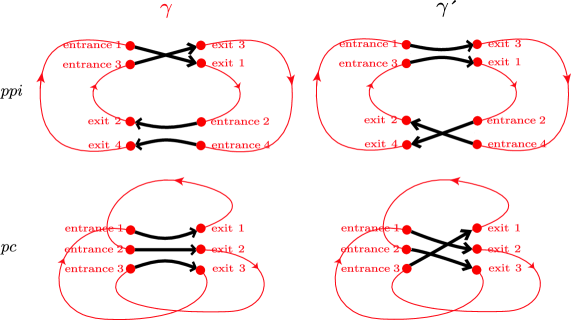
Abbildung 1: Connections between entrance and exit ports for orbit pairs $(\gamma,\gamma^{\prime})$ of structures ppi and pc, existing both for systems with and without time-reversal invariance.

Interestingly, no qualifying $P_{\rm enc}$’s exist for even $L-V+1=n$. For example, the only candidate for $n=2$ would be $P_{\rm enc}=\left({1\atop 2}{2\atop 1}\right)$, describing reconnections inside an encounter of two parallel orbit stretches $\mathrel{\,\lower 0.6458pt\hbox{\begin{picture}(4.0,3.0)\put(0.0,0.8){\vector(1,0){4.0}}\put(0.0,2.0){\vector(1,0){4.0}} \end{picture}}\,}$. As shown in Fig. 1, the corresponding partner decomposes into two separate periodic orbits (corresponding to the cycles $(1)$ and $(2)$ of $P=P_{\rm loop}P_{\rm enc}=\left({1\atop 1}{2\atop 2}\right)$).

The same happens for all other permutations with $n$ even. This can be proven based on the parities of the permutations involved. A permutation is said to have parity 1 if it can be written as a product of an even number of transpositions (i.e., permutations interchanging two elements and leaving all others invariant), and to be of parity $-1$ if it is a product of an odd number of transpositions. Parity is given by $(-1)^{L-V}$, where $L$ is the number of permuted elements and $V$ the number of cycles, and the parity of a product of permutations equals the product of parities of the factors. Since $P$ and $P_{\rm loop}$ both consist of one single cycle, they are of the same parity. Therefore, $P=P_{\rm loop}P_{\rm enc}$ implies that all allowed $P_{\rm enc}$ need to have parity 1, i.e., $n=L-V+1$ must be odd.

For $n$ odd, the individual numbers $N(\vec{v})$ and $\tilde{N}(\vec{v})$, see Eq. (23), do not vanish, indicating that there are orbit pairs contributing to the odd powers of $\tau$. However, their contributions mutually cancel. We see in Table 1 that the $\tilde{N}(\vec{v})$ related to the same $n$, and thus the corresponding contributions to $K(\tau)$, sum up to zero. That cancellation is the reason why all off-diagonal contributions to the spectral form factor vanish in the unitary case.

For example, the two permutations listed for $n=3$ correspond to the structures ppi and pc introduced in Chapter 3. For ppi, $\gamma^{\prime}$ reconnects entrance and exit ports according to the permutation $P_{\rm enc}=\left({1\atop 3}{2\atop 4}{3\atop 1}{4\atop 2}\right)$; compare Fig. 1. This permutation falls into two 2-cycles $(1,3)$ and $(2,4)$ representing one parallel encounter of stretches 1 and 3, and one parallel encounter of stretches 2 and 4. For ${\it pc}$, the encounter connections can be read off from Fig. 1 as $P_{\rm enc}=\left({1\atop 2}{2\atop 3}{3\atop 1}\right)$, which contains one single 3-cycle $(1,3,2)$ representing a parallel encounter of stretches 1, 3, and 2. We have already seen that the resulting contributions mutually cancel.

In the following Subsections, we will show that the same cancellation occurs for arbitrary $n$. To that end we first need to derive a recursion for $N(\vec{v})$.

3 Recursion relation for $N(\vec{v})$

To find a recursion formula for $N(\vec{v})$, we will imagine one loop (e.g. the one with index $L$) removed from both $\gamma$ and $\gamma^{\prime}$ and study the consequences on the encounters. We shall mostly reason with permutations but the translation rule cycle $\to$ encounter yields an interpretation for orbits. Readers wanting to skip the reasoning may jump to the result in Eq. (14).

As a preparation, let us introduce a subset ${\cal M}(\vec{v},l)$ of ${\cal M}(\vec{v})$ containing all those permutations for which the largest of the permuted numbers, i.e., $L(\vec{v})=\sum_{k}kv_{k}$ belongs to a cycle of length $l$ (it is assumed that $v_{l}>0$). The number of elements in ${\cal M}(\vec{v},l)$ will be denoted by $N(\vec{v},l)$. One can show that the sizes of ${\cal M}(\vec{v})$ and ${\cal M}(\vec{v},l)$ are related as

$$N(\vec{v},l)=\frac{lv_{l}}{L(\vec{v})}N(\vec{v})\,.$$ (2)

To derive (2), we use that all $P_{\rm enc}\in{\cal M}(\vec{v})$ can be brought to the form required for ${\cal M}(\vec{v},l)$ by applying a cyclic permutation. We have to consider the cycle representation of $P_{\rm enc}$, and rename each element $a$ as $(a+\Delta a)\mod L$ with $\Delta a$ fixed. For each $\Delta a$, a different element of $P_{\rm enc}$ will be renamed as $L$. We are interested only in those cyclic permutations which place $L$ inside an $l$-cycle and therefore lead to a member of ${\cal M}(\vec{v},l)$. For each $P_{\rm enc}\in{\cal M}(\vec{v})$, there are $lv_{l}$ such possibilities. Since each member of ${\cal M}(\vec{v},l)$ can be accessed using $L(\vec{v})$ different cyclic permutations, we have $lv_{l}N(\vec{v})=L(\vec{v})N(\vec{v},l)$ and thus (2).

Mapping between permutations

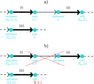
Abbildung 2: a) Thick lines: Three encounter stretches of an orbit $\gamma^{\prime}$, connecting entrance ports to exit ports. The stretches depicted may belong to either the same or different encounters. Thin line: Loop connecting exit $L-1$ to exit $L$. In b), the above loop is removed, and exit $L$ is renamed as exit $L-1$.

We need a mapping that leads from a given permutation $P_{\rm enc}\in{\cal M}(\vec{v},l)$ to a permutation $Q_{\rm enc}$ of smaller size, with a different cycle structure. To motivate such a mapping, we formally remove one orbit loop of $\gamma$ and $\gamma^{\prime}$. Let us consider the sequence of entrance and exit ports traversed by the partner orbit $\gamma^{\prime}$, as depicted in Fig. 2a. Entrance ports are connected to exit ports through encounter stretches visualized by thick arrows, e.g. leading (i) from entrance $P_{\rm enc}^{-1}(L-1)$ to exit $L-1$, (ii) from entrance $L$ to exit $P_{\rm enc}(L)$, and (iii) from entrance $P_{\rm enc}^{-1}(L)$ to exit $L$. It is easy to show that the stretches (i)-(iii) may not mutually coincide. In contrast, loops – depicted by thin arrows – lead from exit ports to entrance ports, e.g. from exit $L-1$ to entrance $L$.

We now remove the orbit loop with index $L$ leading from exit $L-1$ to entrance $L$ (including the latter ports!). The remaining exit $L$ has to be renamed as exit $L-1$; see Fig. 2b. As a consequence, entrance $P_{\rm enc}^{-1}(L-1)$ is now connected to exit $P_{\rm enc}(L)$, and entrance $P_{\rm enc}^{-1}(L)$ is connected to exit $L-1$. All other intra-encounter connections remain unaffected. The resulting encounter permutation $Q_{\rm enc}$ thus acts on the elements $a=1,2,\ldots,L-1$ as

$$Q_{\rm enc}(a)=\begin{cases}P_{\rm enc}(L)&\text{if $a=P_{\rm enc}^{-1}(L-1)$}\\ L-1&\text{if $a=P_{\rm enc}^{-1}(L)$}\\ P_{\rm enc}(a)&\text{otherwise}\;.\end{cases}$$ (3)

Since we only removed an orbit loop, both $\gamma$ and $\gamma^{\prime}$ remain connected periodic orbits. The ordering of entrance ports in $\gamma$ and $\gamma^{\prime}$ is given by single-cycle permutations $Q^{\gamma}=Q_{\rm loop}$ and $Q$, obtained from $P^{\gamma}=P_{\rm loop}$ and $P$ by simply removing the entrance port $L$; in particular $Q_{\rm loop}=(1,2,\ldots,L-1)$. Thus, $Q_{\rm enc}$ automatically satisfies the restriction of producing a single-cycle permutation $Q=Q_{\rm loop}Q_{\rm enc}$.

We need to connect the cycle structures of $Q_{\rm enc}$ and $P_{\rm enc}$, in particular the corresponding vectors $\vec{v}$ and the placement of the largest permuted number. To do so, we shall assume $P_{\rm enc}\in{\cal M}(\vec{v},l)$ with arbitrary $l$ and distinguish between two cases. (For the unitary form factor, we only need $l=2$ and the first case, but the remaining considerations are an essential preparation for the treatment of time-reversal invariant systems.)

First case: $L-1$ and $L$ belong to different cycles

Let us first consider the case that the element $L-1$ of the permutation $P_{\rm enc}$ belongs to a different cycle than $L$, say a $k$-cycle. ($k$ may be equal to $l$.) Hence, $P_{\rm enc}$ has the form

$$P_{\rm enc}=[\ldots](L-1,a_{2},a_{3},\ldots a_{k})(L,b_{2},b_{3},\ldots b_{l})$$ (5)

where the two aforementioned cycles are written in round brackets, and $[\ldots]$ stands for all other cycles. Then, the $Q_{\rm enc}$ given in (3) differs from $P_{\rm enc}$ by mapping $P_{\rm enc}^{-1}(L-1)=a_{k}$ to $P_{\rm enc}(L)=b_{2}$, and $P_{\rm enc}^{-1}(L)=b_{l}$ to $L-1$. It follows that the above $k$- and $l$-cycles of $P_{\rm enc}$ merge to a $(k+l-1)$-cycle of $Q_{\rm enc}$. We may write

$$Q_{\rm enc}=[\ldots](L-1,a_{2},a_{3},\ldots a_{k},b_{2},b_{3},\ldots b_{l})$$ (6)

where $[\ldots]$ is the same as in Eq. (5). Compared to $P_{\rm enc}$, $Q_{\rm enc}$ has one $k$-cycle and one $l$-cycle less, but one additional $(k+l-1)$-cycle. The changed “vector” with $v_{k}\to v_{k}-1,v_{l}\to v_{l}-1,v_{k+l-1}\to v_{k+l-1}+1$ will be denoted as $\vec{v}^{\;[k,l\to k+l-1]}$. In general, $\vec{v}^{[\alpha_{1},\ldots,\alpha_{m}\to\beta_{1},\ldots,\beta_{n}]}$, $m\geq 0$, $n\geq 0$ denotes the vector obtained from $\vec{v}$ if we decrease all $v_{\alpha_{i}}$ by one, increase all $v_{\beta_{i}}$ by one, and leave all other components unchanged. If one number appears several times on either the left or the right hand side, the corresponding component of $\vec{v}$ is respectively decreased or increased by the number of occurrences; if no $\beta_{i}$ appear on the right-hand side, no components of $\vec{v}$ are increased.

The permutation $Q_{\rm enc}$ belongs to the subset ${\cal M}(\vec{v}^{[k,l\to k+l-1]},k+l-1)$ since the largest permuted number $L-1$ is included in a cycle with the length $k+l-1$. We have seen that the additional restriction of $Q=Q_{\rm loop}Q_{\rm enc}$ being single-cycle is satisfied by construction.

Each $P_{\rm enc}$ of the form (5) (with $k$ and $l$ fixed) generates one member of the set ${\cal M}(\vec{v}^{[k,l\to k+l-1]},k+l-1)$. Vice versa, for fixed $k$ the $Q_{\rm enc}$ given in Eq. (6) uniquely determines one $P_{\rm enc}$ as given in Eq. (5): For each $Q_{\rm enc}$, we may simply read off the elements $a_{2},\ldots,a_{k},b_{2},\ldots,b_{l}$ by comparison with (6) and then rearrange them to form a permutation $P_{\rm enc}$ as in (5). Hence, there are

$$N(\vec{v}^{[k,l\to k+l-1]},k+l-1)\,$$ (7)

members of ${\cal M}(\vec{v},l)$ structured like Eq. (5).

Physically, the present scenario is analogous to the merger of a $k$- and an $l$-encounter into a $(k+l-1)$-encounter, by shrinking away an intervening loop.

Second case: $L-1$ and $L$ belong to the same cycle

We now turn to the second scenario where $L$ and $L-1$ belong to the same $l$-cycle of $P_{\rm enc}$. In this case, the element $L$ has to follow $L-1$ after a certain number $m$ of iterations of $P_{\rm enc}$, i.e., $L=P_{\rm enc}^{m}(L-1)$. The number $m$ must satisfy $1\leq m\leq l-2$; $m=l-1$, and thus $L=P_{\rm enc}^{l-1}(L-1)=P_{\rm enc}^{-1}(L-1)$, is excluded since otherwise the stretches (i) and (ii) of Fig. 2a would coincide. The permutation $P_{\rm enc}$ will be of the form

$$P_{\rm enc}=[\ldots](L-1,a_{2},a_{3},\ldots a_{m},L,a_{m+2},\ldots,a_{l})\,.$$ (8)

According to Eq. (3), $Q_{\rm enc}$ differs from $P_{\rm enc}$ by mapping $P_{\rm enc}^{-1}(L-1)=a_{l}$ to $P_{\rm enc}(L)=a_{m+2}$ and mapping $P_{\rm enc}^{-1}(L)=a_{m}$ to $L-1$. The permutation $Q_{\rm enc}$ thus reads

$$Q_{\rm enc}=[\ldots](L-1,a_{2},a_{3},\ldots a_{m})(a_{m+2},\ldots,a_{l})\,.$$ (9)

Here, the $l$-cycle of $P_{\rm enc}$ is broken up into two cycles, with the lengths $m$ and $l-m-1$. Since the largest number $L-1$ is included in an $m$-cycle, $Q_{\rm enc}$ belongs to ${\cal M}(\vec{v}^{[l\to m,l-m-1]},m)$.

In contrast to the first scenario, there are typically several $P_{\rm enc}$ producing the same $Q_{\rm enc}$. Indeed Eq. (9) would not only result from Eq. (8), but also from all $l-m-1$ permutations $P_{\rm enc}$ obtained by cyclic permutation of the last elements $a_{m+2},\ldots,a_{l}$ in Eq. (8). Besides, $[\ldots]$ in $P_{\rm enc}$ contains $v_{l-m-1}$ cycles of length $l-m-1$. If we transpose the content of one of these cycles with the subsequence $a_{m+2},\ldots,a_{l}$ in Eq. (8), the resulting $P_{\rm enc}$ will lead to the same $Q_{\rm enc}$; in any of these cases $Q_{\rm enc}$ will contain the $v_{l-m-1}$ cycles of length $l-m-1$ included in the $[\ldots]$ of Eq. (8) and one additional such cycle given by $(a_{m+2},\ldots,a_{l})$. Thus, there are $(l-m-1)(v_{l-m-1}+1)$ permutations $P_{\rm enc}$ producing the same $Q_{\rm enc}$, due to the $v_{l-m-1}+1$ possibilities for transposing (or keeping) $a_{m+2},\ldots,a_{l}$, and $l-m-1$ possibilities for cyclicly permuting them. Consequently, for each $m$ the subset of elements $P_{\rm enc}\in{\cal M}(\vec{v},l)$ structured like Eq. (8) is $(l-m-1)(v_{l-m-1}+1)$ times larger than ${\cal M}(\vec{v}^{[l\to m,l-m-1]},m)$, i.e., it has the size

$$(l-m-1)(v_{l-m-1}+1)N(\vec{v}^{[l\to m,l-m-1]},m)\,.$$ (10)

The second scenario, too, has an interesting physical interpretation. If $L-1$ and $L$ both belong to the same $l$-cycle, they must correspond to two subsequent parallel stretches of the same encounter. If we remove the intervening orbit loop, these stretches will overlap; this overlap will be studied in more detail in Appendix 11.C.

Resulting recursion

We have decomposed ${\cal M}(\vec{v},l)$ into several subsets of size $N(\vec{v}^{[k,l\to k+l-1]},k+l-1)$, $k\geq 2$, and further subsets of size $(l-m-1)(v_{l-m-1}+1)N(\vec{v}^{[l\to m,l-m-1]},m)$, with $m=1,\ldots,l-2$. The size of ${\cal M}(\vec{v},l)$ thus reads

$$N(\vec{v},l) = \sum_{k\geq 2}N(\vec{v}^{[k,l\to k+l-1]},k+l-1)$$ (11)

$$+ \sum_{m=1}^{l-2}(l-m-1)(v_{l-m-1}+1)N(\vec{v}^{[l\to m,l-m-1]},m)\,.$$

Using $N(\vec{v},l)=\frac{lv_{l}}{L}N(\vec{v})$, we find the desired recursion for the number of structures $N(\vec{v})$,

$$\frac{lv_{l}}{L}N(\vec{v}) = \sum_{k\geq 2}\frac{(k+l-1)(v_{k+l-1}+1)}{L-1}N(\vec{v}^{[k,l\to k+l-1]})$$

$$+ \sum_{m=1}^{l-2}\frac{(l-m-1)(v_{l-m-1}+1)mv_{m}^{[l\to m,l-m-1]}}{L-1}N(\vec{v}^{[l\to m,l-m-1]})\,.$$

Alternatively, we may formulate our recursion in terms of the numbers $\tilde{N}(\vec{v})=N(\vec{v})\frac{(-1)^{V}\prod_{l}l^{v_{l}}}{L(\vec{v})}$ determining the contributions to the spectral form factor,

$$v_{l}\tilde{N}(\vec{v})+\sum_{k\geq 2}(v_{k+l-1}+1)k\tilde{N}(\vec{v}^{[k,l\to k+l-1]})$$

$$+\sum_{m=1}^{l-2}(v_{l-m-1}+1)v_{m}^{[l\to m,l-m-1]}\tilde{N}(\vec{v}^{[l\to m,l-m-1]})=0\,.$$ (13)

Note that $v_{k+l-1}+1=v_{k+l-1}^{[k,l\to k+l-1]}$. Of course, the $k$th summand vanishes if there are no $k$-cycles present, i.e., if $v_{k}=0$ and thus formally $v_{k}^{[k,l\to k+l-1]}=-1$.

To determine the form factor for systems without time-reversal invariance, we need only the special case $l=2$. In this case, our recursion strongly simplifies,

$$v_{2}\tilde{N}(\vec{v})+\sum_{k\geq 2}v_{k+1}^{[k,2\to k+1]}k\tilde{N}(\vec{v}^{[k,2\to k+1]})=0\,,$$ (14)

since only the first of the two above scenarios is possible. That is, a 2-cycle may only merge with a $k$-cycle to form a $(k+1)$-cycle, but not split into two separate cycles. Recall that $\vec{v}^{[k,2\to k+1]}$ is obtained from $\vec{v}$ by decreasing both $v_{k}$ and $v_{2}$ by one, and increasing $v_{k+1}$ by one.

4 Spectral form factor

We had expressed the Taylor coefficients of the form factor as a sum over the combinatorial numbers $\tilde{N}(\vec{v})$,

$$K_{n}=\frac{1}{(n-2)!}\sum_{\vec{v}}^{\nu(\vec{v})=n}\tilde{N}(\vec{v})\,,\quad n\geq 2\,,$$ (15)

see Eq. (22), where the sum runs over all $\vec{v}$ with $v_{1}=0$ which satisfy $\nu(\vec{v})\equiv L(\vec{v})-V(\vec{v})+1=n$; the condition $v_{1}=0$ is not written out explicitly. Our recursion relation for $\tilde{N}(\vec{v})$ now translates into a recursion for $K_{n}$, albeit a trivial one in the unitary case, implying that all $K_{n}$ except $K_{1}$ vanish. (Alternatively, one may use a rather involved explicit formula for $N(\vec{v})$ [46].)

To show this, consider the recursion (14) for $\tilde{N}(\vec{v})$ and sum over $\vec{v}$ as above

$$\sum_{\vec{v}}^{\nu(\vec{v})=n}\left(v_{2}\tilde{N}(\vec{v})+\sum_{k\geq 2}v_{k+1}^{[k,2\to k+1]}k\tilde{N}(\vec{v}^{[k,2\to k+1]})\right)=0\,.$$ (16)

Each of the sums

$$\sum_{\vec{v}}^{\nu(\vec{v})=n}v_{k+1}^{[k,2\to k+1]}\tilde{N}(\vec{v}^{[k,2\to k+1]})$$ (17)

may be transformed into a sum over the argument of $\tilde{N}$, i.e., $\vec{v}^{\prime}=\vec{v}^{[k,2\to k+1]}$. The vectors $\vec{v}^{\prime}$ must satisfy three restrictions. First, by definition we must have $v_{k+1}^{\prime}\geq 1$. However, this restriction may be dropped because due to the prefactor $v^{\prime}_{k+1}$ terms with $v^{\prime}_{k+1}=0$ do not contribute to (17). Second, $\nu(\vec{v})=n$ implies that $\nu(\vec{v}^{\prime})=n$, since going from $\vec{v}$ to $\vec{v}^{\prime}$ decreases both $L$ and $V$ by one and thus leaves $\nu$ invariant. Third, just like $\vec{v}$ the vectors $\vec{v}^{\prime}$ must fulfill the implicit condition $v_{1}^{\prime}=0$. We thus have to sum over all $\vec{v}^{\prime}$ with $\nu(\vec{v}^{\prime})=n$ (and $v_{1}^{\prime}=0$), and simplify (17) as in

$$\sum_{\vec{v}}^{\nu(\vec{v})=n}v_{k+1}^{[k,2\to k+1]}\tilde{N}(\vec{v}^{[k,2\to k+1]})=\sum_{\vec{v}^{\prime}}^{\nu(\vec{v}^{\prime})=n}v^{\prime}_{k+1}\tilde{N}(\vec{v}^{\prime})\,.$$ (18)

Applying this rule to all terms in Eq. (16) and dropping the primes, we obtain

$$\sum_{\vec{v}}^{\nu(\vec{v})=n}\Big{(}v_{2}+\sum_{k\geq 2}v_{k+1}k\Big{)}\tilde{N}(\vec{v})=0\,.$$ (19)

Since the term in parentheses is just $\sum_{l\geq 2}v_{l}(l-1)=L-V=\nu-1=n-1$ we have

$$(n-1)\sum_{\vec{v}}^{\nu(\vec{v})=n}\tilde{N}(\vec{v})=(n-1)!\,K_{n}=0\,,$$ (20)

for all $n\geq 2$.

We see that all Taylor coefficients except $K_{1}$ vanish: orbit pairs differing in encounters yield no net contribution to the form factor, but mutually compensate. Only the “diagonal” orbit pairs remain, and indeed lead to the same small-time form factor as predicted by random-matrix theory for the GUE.

2 Orthogonal case

1 Structures and permutations

For time-reversal invariant systems, too, structures of orbit pairs can be related to permutations. Given time-reversal invariance, the partners of an orbit $\gamma$ may involve loops of both $\gamma$ and its time-reversed $\overline{\gamma}$. All permutations used will thus simultaneously describe $\gamma$ and $\overline{\gamma}$, or both one partner $\gamma^{\prime}$ and its time-reversed $\overline{\gamma^{\prime}}$. Compared to the unitary case, the permuted elements will be doubled in number.

The above orbits differ in a certain number of encounters. Again, the encounter stretches of $\gamma$ will be numbered in order of traversal as $1,2,\ldots,L$. Each of these stretches leads from an entrance to an exit port, both to be labelled by the same index as the corresponding encounter stretch. The encounter stretches of $\overline{\gamma}$ are time-reversed with respect to those of $\gamma$, and will be labelled by $\overline{1},\overline{2},\ldots,\overline{L}$, with $\overline{a}$ denoting the time-reversed of the $a$th stretch of $\gamma$. Stretch $\overline{a}$ of $\overline{\gamma}$ leads from entrance port $\overline{a}$ to exit port $\overline{a}$. These ports coincide with those of $\gamma$ in configuration space, but are time-reversed and have entrance and exit swapped. The exit port $\overline{a}$ of $\overline{\gamma}$ is the time-reversed of the entrance port $a$ of $\gamma$, and entrance port $\overline{a}$ of $\overline{\gamma}$ is the time-reversed of the exit port $a$ of $\gamma$. See Fig. 3 for the example of a 2-encounter.

The intra-encounter connections of $\gamma$ and $\overline{\gamma}$ are represented by the trivial permutation $P_{\rm enc}^{\gamma}=\left({1\atop 1}{2\atop 2}{\ldots\atop\ldots}{L\atop L}{\overline{1}\atop\overline{1}}{\overline{2}\atop\overline{2}}{\ldots\atop\ldots}{\overline{L}\atop\overline{L}}\right)$ indicating that each entrance port (upper line) is connected to an exit (lower line) with the same index.

The corresponding connections in $\gamma^{\prime}$, $\overline{\gamma^{\prime}}$ are given by a different permutation $P_{\rm enc}$. In the example of a Sieber/Richter pair, Fig. 3, the partner $\gamma^{\prime}$ connects the entrance 1 of $\gamma$ to the exit $\overline{2}$ of $\overline{\gamma}$, and the entrance $\overline{1}$ of $\overline{\gamma}$ to the exit 2 of $\gamma$. The time-reversed partner $\overline{\gamma^{\prime}}$ connects the entrance $\overline{2}$ to exit 1, and entrance 2 to exit $\overline{1}$. We thus write $P_{\rm enc}=\left({1\atop\overline{2}}{2\atop\overline{1}}{\overline{1}\atop 2}{\overline{2}\atop 1}\right)$. (Note that the sequence of columns in $P_{\rm enc}$ may be ordered arbitrarily!)

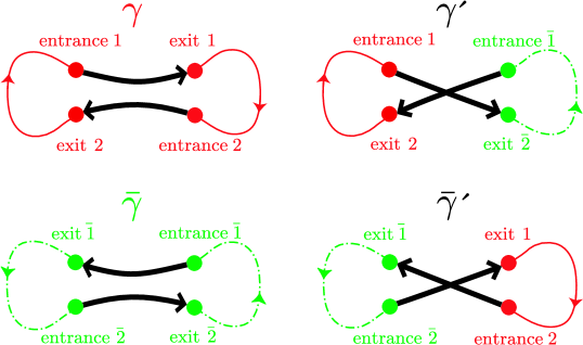
Abbildung 3: Entrance-to-exit connections for a Sieber/Richter pair, in an orbit $\gamma$, its time-reversed $\overline{\gamma}$, and the partners $\gamma^{\prime},\overline{\gamma^{\prime}}$. Loops of $\gamma$ are depicted by full lines, loops of $\overline{\gamma}$ by dash-dotted lines.

In general, time-reversal invariance imposes the following restriction on $P_{\rm enc}$: If a stretch connects entrance $a$ to exit $b$, the time-reversed stretch must lead from entrance $\overline{b}$ (the time-reversed of exit $b$) to exit $\overline{a}$ (the time-reversed of entrance $a$). This restriction also applies if $a$ or $b$ belong to $\overline{\gamma}$ and thus contain an overbar, e.g. $a=\overline{p}$; we then define $\overline{\overline{p}}=p$. In any case, if $P_{\rm enc}$ maps $a$ to $b$, it has to map $\overline{b}$ to $\overline{a}$, with $a,b$ standing for elements out of $1,\ldots,L,\overline{1},\ldots,\overline{L}$. This restriction on $P_{\rm enc}$ will be referred to as “time-reversal covariance”. Writing ${\cal T}(a)\equiv\overline{a}$, a given $P_{\rm enc}$ is time-reversal covariant if ${\cal T}P_{\rm enc}{\cal T}=P_{\rm enc}^{-1}$ such that ${\cal T}P_{\rm enc}{\cal T}(b)={\cal T}P_{\rm enc}(\overline{b})={\cal T}(\overline{a})=a=P_{\rm enc}^{-1}(b)$ holds for arbitrary $b$. Obviously, for Sieber/Richter pairs the $P_{\rm enc}$ given above is time-reversal covariant.

Again, $l$-encounters are related to cycles of $P_{\rm enc}$. If we take into account both $\gamma$ and $\overline{\gamma}$, each encounter contains $2l$ stretches – $l$ stretches belonging to $\gamma$ and $l$ stretches belonging to $\overline{\gamma}$. Alternatively, the $2l$ stretches may be grouped into $l$ stretches pointing “from left to right” (i.e., parallel to the first stretch inside $\gamma$ belonging to the corresponding encounter), and $l$ stretches leading from right to left. The stretches of each group are mutually close in phase space, and approximately time-reversed with respect to those of the other group. The two groups may mix stretches of $\gamma$ and $\overline{\gamma}$; only for parallel encounters all stretches of $\gamma$ point from left to right and all stretches of $\overline{\gamma}$ point from right to left. The partner orbits $\gamma^{\prime}$, $\overline{\gamma^{\prime}}$ can be obtained by reconnecting stretches inside these two groups, without having to revert stretches or ports in time.

Each of the two groups corresponds to one $l$-cycle of $P_{\rm enc}$. To show this, we reason similarly to Subsection 1. Two stretches with labels $a$ and $P_{\rm enc}(a)$ must belong to the same group, such that the entrance of $a$ can be connected to the exit of $P_{\rm enc}(a)$. Starting with an arbitrary label $a$, iteration yields a complete list $a,P_{\rm enc}(a),P_{\rm enc}^{2}(a),P_{\rm enc}^{3}(a),\ldots$ of stretches involved in mutual reconnections and thus belonging to the same group. After $l$ iterations, we are led back to the initial element $a$ and thus obtain an $l$-cycle. Consequently, each $l$-encounter corresponds to a pair of “twin” $l$-cycles. (An encounter associated with more cycles would decompose into several encounters with independent reconnections, similarly to the encounters depicted in Fig. 1c for the unitary case.)

The stretches of both groups are mutually time-reversed. If one group contains a stretch leading from entrance $a_{i}$ to exit $a_{i+1}$, the stretch leading from entrance $\overline{a_{i+1}}$ to exit $\overline{a_{i}}$ is part of the other group. This behavior is mirrored by the two associated cycles, which must be of “mutually time-reversed” form $(a_{1},a_{2},\ldots,a_{l-1},a_{l})$, $(\overline{a_{l}},\overline{a_{l-1}},\ldots,\overline{a_{2}},\overline{a_{1}})$. For example, the permutation $P_{\rm enc}=\left({1\atop\overline{2}}{2\atop\overline{1}}{\overline{1}\atop 2}{\overline{2}\atop 1}\right)$ describing reconnections in Sieber/Richter pairs has two mutually time-reversed cycles $(1,\overline{2})$ and $(2,\overline{1})$, with $(1,\overline{2})$ representing the stretches leading from left to right, and $(2,\overline{1})$ representing the stretches directed from right to left.

The orbit loops are associated with $P_{\rm loop}=\left({1\atop 2}{2\atop 3}{\ldots\atop\ldots}{L\atop 1}{\overline{2}\atop\overline{1}}{\overline{3}\atop\overline{2}}{\ldots\atop\ldots}{\overline{1}\atop\overline{L}}\right)$, since if one loop of $\gamma$ leads from the exit of the $(a-1)$-st stretch to the entrance of the $a$-th one, its time-reversed must go from exit $\overline{a}$ to entrance $\overline{a-1}$. The loops remain unchanged in the partner orbits $\gamma^{\prime}$, $\overline{\gamma^{\prime}}$ and are thus always described by the same $P_{\rm loop}$.

The product $P^{\gamma}=P_{\rm loop}P_{\rm enc}^{\gamma}=P_{\rm loop}$ specifies the ordering of entrance ports along the two orbits $\gamma$ and $\overline{\gamma}$. That $P^{\gamma}$ has two cycles $(1,2,\ldots,L)$ and $(\overline{L},\overline{L-1},\ldots,\overline{1})$, one each for $\gamma$ and $\overline{\gamma}$.

The ordering of entrance ports along the partners $\gamma^{\prime}$, $\overline{\gamma^{\prime}}$ is given by the product $P=P_{\rm loop}P_{\rm enc}$. To obtain two connected partner orbits $\gamma^{\prime}$ and $\overline{\gamma^{\prime}}$, we now have to demand $P$ to consist of only two $L$-cycles, listing the entrance ports in $\gamma^{\prime}$ and $\overline{\gamma^{\prime}}$, respectively. This provides a restriction on $P_{\rm enc}$ analogous to the unitary case.

The two cycles of $P$ are not independent. The second cycle containing the entrance ports of $\overline{\gamma^{\prime}}$ can also be interpreted as the list of exit ports of $\gamma^{\prime}$, time-reversed and written in reverse order. Since an entrance $a_{i}$ is connected by a loop to the exit $b_{i}\equiv P_{\rm loop}^{-1}(a_{i})$, the two cycles of $P$ must be of the form $(a_{1},a_{2},\ldots,a_{L})$ and $(\overline{b_{L}},\overline{b_{L-1}},\ldots,\overline{b_{1}})$. It is easy to show that this form follows immediately from time-reversal covariance and the existence of two cycles, and thus does not provide a further restriction on $P_{\rm enc}$.

Each of the permutations $P_{\rm enc}$ corresponds to one structure of orbit pairs as defined in Section 4. The division of labels $1,2,\ldots,L,\overline{1},\overline{2},\ldots,\overline{L}$ into pairs of cycles determines how stretches are divided among encounters. By further dividing labels (and thus stretches) of one encounter in two “mutually time-reversed” cycles, we fix the mutual orientation of stretches inside each encounter. Finally, the ordering of labels inside cycles determines the reconnections leading to $\gamma^{\prime}$, $\overline{\gamma^{\prime}}$ which have to be connected periodic orbits if $P$ falls in two $L$-cycles.

To establish a recursion for the numbers of structures $N(\vec{v})$, we may consider the set ${\cal M}(\vec{v})$ of permutations $P_{\rm enc}$ acting on $1,2,\ldots,L,\overline{1},\overline{2},\ldots,\overline{L}$ which (i) are time-reversal covariant, (ii) have $v_{l}$ pairs of $l$-cycles for all $l\geq 2$, and (iii) lead to a permutation $P=P_{\rm loop}P_{\rm enc}$ consisting of two $L$-cycles. Each element $P_{\rm enc}$ of the set ${\cal M}(\vec{v})$ stands for one of the structures related to $\vec{v}$. We need to calculate the number $N(\vec{v})$ of elements of ${\cal M}(\vec{v})$.

2 Examples

order	$\vec{v}$	$L$	$V$	$N(\vec{v})$	$\tilde{N}(\vec{v})$	contribution
$\tau^{2}$	$(2)^{1}$	2	1	1	$-1$	$-2\tau^{2}$
					$-1$	$-2\tau^{2}$
$\tau^{3}$	$(2)^{2}$	4	2	5	5	$10\tau^{3}$
	$(3)^{1}$	3	1	4	$-4$	$-8\tau^{3}$
					1	2$\tau^{3}$
$\tau^{4}$	$(2)^{3}$	6	3	41	$-\frac{164}{3}$	$-\frac{164}{3}\tau^{4}$
	$(2)^{1}(3)^{1}$	5	2	60	72	$72\tau^{4}$
	$(4)^{1}$	4	1	20	$-20$	$-20\tau^{4}$
					$-\frac{8}{3}$	$-\frac{8}{3}\tau^{4}$
$\tau^{5}$	$(2)^{4}$	8	4	509	1018	$\frac{1018}{3}\tau^{5}$
	$(2)^{2}(3)^{1}$	7	3	1092	$-1872$	$-624\tau^{5}$
	$(2)^{1}(4)^{1}$	6	2	504	672	$224\tau^{5}$
	$(3)^{2}$	6	2	228	342	$114\tau^{5}$
	$(5)^{1}$	5	1	148	$-148$	$-\frac{148}{3}\tau^{5}$
					12	4$\tau^{5}$
$\tau^{6}$	$(2)^{5}$	10	5	8229	$-\frac{131664}{5}$	$-\frac{10972}{5}\tau^{6}$
	$(2)^{3}(3)^{1}$	9	4	23160	61760	$\frac{15440}{3}\tau^{6}$
	$(2)^{2}(4)^{1}$	8	3	12256	$-24512$	$-\frac{6128}{3}\tau^{6}$
	$(2)^{1}(3)^{2}$	8	3	10960	$-24660$	$-2055\tau^{6}$
	$(2)^{1}(5)^{1}$	7	2	5236	7480	$\frac{1870}{3}\tau^{6}$
	$(3)^{1}(4)^{1}$	7	2	4396	7536	$628\tau^{6}$
	$(6)^{1}$	6	1	1348	$-1348$	$-\frac{337}{3}\tau^{6}$
					$-\frac{384}{5}$	$-\frac{32}{5}\tau^{6}$

Tabelle 2: Permutations, and thus structures of orbit pairs, giving rise to orders $\tau^{2}$ to $\tau^{6}$ of the form factor, for systems with time-reversal invariance; notation as in Table 1. The results coincide with the predictions of RMT for the GOE.

Again, the numbers $N(\vec{v})$ can be determined by numerically counting permutations. From the results shown in Table 2, we see that indeed the form factor of the Gaussian Orthogonal Ensemble is reproduced semiclassically.

The $\tau^{2}$ contribution comes from pairs of orbits differing in one antiparallel 2-encounter, with the “encounter permutation” $P_{\rm enc}=\left({1\atop\overline{2}}{2\atop\overline{1}}{\overline{1}\atop 2}{\overline{2}\atop 1}\right)$.

We have already seen that the $\tau^{3}$ contribution originates from four structures related to 3-encounters and five structures related to pairs of 2-encounters. If all encounters are parallel (structures ppi and pc), the partner $\gamma^{\prime}$ is obtained by reconnecting the ports of $\gamma$, and determined by the permutations given in Subsection 2. If we also want to describe the time-reversed orbits $\overline{\gamma}$ and $\overline{\gamma^{\prime}}$, we have to extend the permutations given as required by time-reversal covariance, i.e., each mapping $a\to b$ must be complemented by a connection $\overline{b}\to\overline{a}$. This yields $P_{\rm enc}=\left({1\atop 3}{2\atop 4}{3\atop 1}{4\atop 2}{\overline{1}\atop\overline{3}}{\overline{2}\atop\overline{4}}{\overline{3}\atop\overline{1}}{\overline{4}\atop\overline{2}}\right)=(1,3)(\overline{3},\overline{1})(2,4)(\overline{4},\overline{2})$ for ppi and $P_{\rm enc}=\left({1\atop 2}{2\atop 3}{3\atop 1}{\overline{1}\atop\overline{3}}{\overline{2}\atop\overline{1}}{\overline{3}\atop\overline{2}}\right)=(1,2,3)(\overline{3},\overline{2},\overline{1})$ for pc.

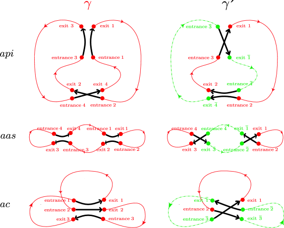
Abbildung 4: Connections between entrance and exit ports of orbit pairs $(\gamma,\gamma^{\prime})$ existing only for systems with time-reversal invariance. The partner $\gamma^{\prime}$ mixes loops of $\gamma$ (full lines) and its time-reversed $\overline{\gamma}$ (dash-dotted lines). (See 4 for orbit pairs which do not require time-reversal invariance.) For each of the families api, aas, and ac we depicted one of several equivalent structures; the others are obtained by cyclic permutation of the port labels.

For the remaining cases api, aas, and ac, the original orbit $\gamma$ and one of its partners $\gamma^{\prime}$ are depicted in Fig. 4; $\gamma^{\prime}$ includes ports and loops of both $\gamma$ and its time-reversed $\overline{\gamma}$ (with loops respectively depicted by full and dash-dotted lines). Similarly to ppi, each parallel encounter of two stretches $a$ and $b$ leads to two cycles $(a,b)(\overline{b},\overline{a})$ representing the stretches $a$, $b$ pointing from left to right, and the stretches $\overline{b}$, $\overline{a}$ pointing from right to left. In contrast, an antiparallel 2-encounter of a stretch $a$ and a later stretch $b$ leads to $(a,\overline{b})(b,\overline{a})$ since $a$ and $\overline{b}$ are directed from left to right, whereas $b$ and $\overline{a}$ are directed from right to left (like in the above example of a Sieber/Richter pair). The two structures related to api (Section 1) can now immediately be translated into permutations. A parallel encounter of stretches 1 and 3, complemented with an antiparallel encounter of stretches 2 and 4, is represented by the permutation $P_{\rm enc}=(1,3)(\overline{3},\overline{1})(2,\overline{4})(4,\overline{2})=\left({1\atop 3}{2\atop\overline{4}}{3\atop 1}{4\atop\overline{2}}{\overline{1}\atop\overline{3}}{\overline{2}\atop 4}{\overline{3}\atop\overline{1}}{\overline{4}\atop 2}\right)$. Indeed, Fig. 4 shows that $\gamma^{\prime}$ connects the entrance and exit ports as $3\to 1$, $2\to\overline{4}$, $\overline{3}\to\overline{1}$, and $\overline{4}\to 2$; the remaining connections belong to $\overline{\gamma^{\prime}}$. Different numbering of stretches leads to a different structure. That structure corresponds to the permutation $P_{\rm enc}=(1,\overline{3})(3,\overline{1})(2,4)(\overline{4},\overline{2})=\left({1\atop\overline{3}}{2\atop 4}{3\atop\overline{1}}{4\atop 2}{\overline{1}\atop 3}{\overline{2}\atop\overline{4}}{\overline{3}\atop 1}{\overline{4}\atop\overline{2}}\right)$, and involves an antiparallel encounter of stretches 1 and 3, and a parallel encounter of stretches 2 and 4.

For aas, antiparallel encounters of stretches 1 and 2, and stretches 3 and 4 lead to the permutation $P_{\rm enc}=(1,\overline{2})(2,\overline{1})(3,\overline{4})(4,\overline{3})=\left({1\atop\overline{2}}{2\atop\overline{1}}{3\atop\overline{4}}{4\atop\overline{3}}{\overline{1}\atop 2}{\overline{2}\atop 1}{\overline{3}\atop 4}{\overline{4}\atop 3}\right)$. Again, the corresponding port connections are displayed in Fig. 4. If we order stretches differently, we obtain $P_{\rm enc}=(1,\overline{4})(4,\overline{1})(2,\overline{3})(3,\overline{2})=\left({1\atop\overline{4}}{2\atop\overline{3}}{3\atop\overline{2}}{4\atop\overline{1}}{\overline{1}\atop 4}{\overline{2}\atop 3}{\overline{3}\atop 2}{\overline{4}\atop 1}\right)$.

Orbit pairs of type ac are described by three equivalent structures and thus permutations. Encounters with stretch 3 antiparallel to stretches 1 and 2 correspond to $P_{\rm enc}=(1,2,\overline{3})(3,\overline{2},\overline{1})=\left({1\atop 2}{2\atop\overline{3}}{3\atop\overline{2}}{\overline{1}\atop 3}{\overline{2}\atop\overline{1}}{\overline{3}\atop 1}\right)$, with cycles respectively standing for the stretches traversed from left to right, and from right to left. Two further permutations are obtained by cyclic permutation of 1,2,3 as well as $\overline{1},\overline{2},\overline{3}$.

3 Excursion: Left and right ports

So far, we have described intra-encounter connections by permutations $P_{\rm enc}$ mapping between entrance and exit ports, labelled by $1,2,\ldots,L,\overline{1},\overline{2},\ldots,\overline{L}$. Alternatively, we might consider permutations $p_{\rm enc}$ describing which left port (upper line) is connected to which right port (lower line). When defining $p_{\rm enc}$, we can identify mutually time-reversed ports coinciding in configuration space and let $p_{\rm enc}$ act only on the $L$ numbers $1,2,\ldots,L$. Such a description would nicely fit with the treatment of Chapter 4. For instance, Eq. (5), stating that stable and unstable coordinates of a piercing point are respectively fixed by the associated left and right ports, could be formulated as $\hat{s}_{j}^{\prime}\approx\hat{s}_{j}$, $\hat{u}_{j}^{\prime}\approx\hat{u}_{p_{\rm enc}(j)}$. Moreover, each $l$-encounter corresponds to just one $l$-cycle of $p_{\rm enc}$ rather than a pair of cycles. However, it is rather difficult to formulate our recursion for $N(\vec{v})$ in terms of $p_{\rm enc}$, which is why we use $P_{\rm enc}$ in the remainder of this thesis.

In the present excursion (which may be skipped by the impatient reader), we will investigate the relation between $p_{\rm enc}$ and $P_{\rm enc}$. To translate between the two, we first consider the special case when all stretches in every encounter are parallel, i.e., directed from left to right in $\gamma$ and from right to left in $\overline{\gamma}$. Then, in the partner $\gamma^{\prime}$ the left port $a$ of $\gamma$ is connected to the right port $p_{\rm enc}(a)$, and in $\overline{\gamma^{\prime}}$ the right port $\overline{p_{\rm enc}(a)}$ of $\overline{\gamma}$ has to be connected to the left port $\overline{a}$. The permutation

$$\tilde{P}_{\rm enc}=\left({1\atop p_{\rm enc}(1)}{\ldots\atop\ldots}\;\;{L\atop p_{\rm enc}(L)}{\overline{p_{\rm enc}(1)}\atop\overline{1}}{\ldots\atop\ldots}\;\;{\overline{p_{\rm enc}(L)}\atop\overline{L}}\right)$$ (21)

thus gives the mapping between entrances (i.e., left ports of $\gamma$ and right ports of $\overline{\gamma}$) and exits (i.e., right ports of $\gamma$ and left ports of $\overline{\gamma}$). Half of the cycles of $\tilde{P}_{\rm enc}$ are those of $p_{\rm enc}$, another half are their time-reversed twins.

Now consider the general case when the motion over some of the encounter stretches is directed from right to left in the original orbit $\gamma$ and from left to right in the time reversed $\overline{\gamma}$; we shall call such stretches “reverted”. Eq. (21) remains true provided the elements in the upper line are interpreted as left ports of $\gamma$ and right ports of $\overline{\gamma}$ (opposite for the lower line). However, we are interested in the encounter permutation $P_{\rm enc}$ which maps entrance to exit ports. For a reverted stretch, e.g., a left port of $\gamma$ is an exit rather than an entrance. To convert this port into an entrance, we have to consider the time-reversed stretch, leading from left to right in $\overline{\gamma}$. To convert all elements in the upper line to entrances and those in the lower line to exits, we have to exchange $a\leftrightarrow\overline{a}$ (i.e., apply time reversal) for all ports of reverted stretches $a$. That exchange of elements amounts to the permutation $\Sigma(a)=\overline{a},\Sigma(\overline{a})=a$ for all reverted stretches while otherwise $\Sigma(a)=a,\Sigma(\overline{a})=\overline{a}$. The encounter permutation $P_{\rm enc}$ is related to $\tilde{P}_{\rm enc}$ by

$$P_{\rm enc}=\Sigma\tilde{P}_{\rm enc}\Sigma\,.$$ (22)

Since $\Sigma$ is idempotent ($\Sigma^{2}=1$) the transformation leading from $\tilde{P}_{\rm enc}$ to $P_{\rm enc}$ is a similarity transformation and thus does not change the cycle structure [44]. Each $l$-cycle of $p_{\rm enc}$ gives rise to two mutually time reversed $l$-cycles of $\tilde{P}_{\rm enc}$ and therefore to two cycles of $P_{\rm enc}$.

4 Recursion relation for $N(\vec{v})$

We are now equipped to establish a recursion relation for $N(\vec{v})$ in much the same way as in the unitary case. We will finally be led to a recursion for $K_{n}$, given in Eq. (52).

First of all, we recover Eq. (2), $N(\vec{v},l)=\frac{v_{l}l}{L(\vec{v})}N(\vec{v})$ using exactly the same arguments as in the unitary case. Each permutation $P_{\rm enc}\in{\cal M}(\vec{v})$ can be converted into a member of ${\cal M}(\vec{v},l)$ by $lv_{l}$ cyclic permutations and each member of ${\cal M}(\vec{v},l)$ is accessed through $L(\vec{v})$ permutations. (The labels with overbar $\overline{1},\overline{2},\ldots,\overline{L}$ have to be permuted in the same way as $1,2,\ldots,L$.)

Mapping between permutations

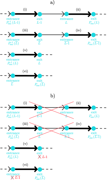
Abbildung 5: a) Thick lines: Six encounter stretches of orbits $\gamma^{\prime}$ and $\overline{\gamma^{\prime}}$, connecting entrance ports to exit ports. The stretches depicted may belong to either the same or different encounters, and to either $\gamma^{\prime}$ or $\overline{\gamma^{\prime}}$. Thin line: Loop connecting exit $L-1$ to entrance $L$, and its time-reversed leading from exit $\overline{L}$ to entrance $\overline{L-1}$. In b), the two above loops are removed, exit $L$ is renamed as exit $L-1$, and entrance $\overline{L}$ is renamed as entrance $\overline{L-1}$.

To define our recursion, we again imagine one orbit loop of $\gamma$ and $\gamma^{\prime}$ removed. Fig. 5 visualizes the ordering of entrance and exit ports along the orbit $\gamma^{\prime}$ and its time-reversed $\overline{\gamma^{\prime}}$, with thick arrows denoting encounter stretches and thin arrows denoting loops. It is easy to show that all six stretches (i)-(vi) depicted in Fig. 5 must be different (except for the special case $P_{\rm enc}(\overline{L-1})=L$ and thus $P_{\rm enc}^{-1}(L-1)=\overline{L}$, which will be investigated later).

Starting from a permutation $P_{\rm enc}$ we may define a permutation $Q_{\rm enc}$ acting on the elements $1,2,\ldots,L-1,\overline{1},\overline{2},\ldots,\overline{L-1}$ by eliminating both the loop leading from exit $L-1$ to entrance $L$ and its time-reversed leading from entrance $\overline{L}$ to exit $\overline{L-1}$. The remaining exit $L$ has to be renamed as exit $L-1$, and entrance $\overline{L}$ is renamed as entrance $\overline{L-1}$. The resulting changes are depicted in Fig. 5b. A look at the remaining thick arrows reveals the new encounter permutation as

$$Q_{\rm enc}(a)=\begin{cases}P_{\rm enc}(L)&\text{if $a=P_{\rm enc}^{-1}(L-1)$}\\ P_{\rm enc}(\overline{L-1})&\text{if $a=P_{\rm enc}^{-1}(\overline{L})$}\\ L-1&\text{if $a=P_{\rm enc}^{-1}(L)$}\\ P_{\rm enc}(\overline{L})&\text{if $a=\overline{L-1}$}\\ P_{\rm enc}(a)&\text{otherwise}\,.\end{cases}$$ (23)

One can easily show that $Q_{\rm enc}$ is a permissible encounter permutation. First, note that the second and fourth line extend Eq. (3) as required to make $Q_{\rm enc}$ time-reversal covariant. The mapping $P_{\rm enc}^{-1}(L-1)\to P_{\rm enc}(L)$ is thus complemented by $\overline{P_{\rm enc}(L)}=P_{\rm enc}^{-1}(\overline{L})\to\overline{P_{\rm enc}^{-1}(L-1)}=P_{\rm enc}(\overline{L-1})$, and $P_{\rm enc}^{-1}(L)\to L-1$ implies $\overline{L-1}\to\overline{P_{\rm enc}^{-1}(L)}=P_{\rm enc}(\overline{L})$. All other mappings $a\to b$ are complemented by $\overline{b}\to\overline{a}$ due to the time-reversal covariance of $P_{\rm enc}$.

Second, by construction reconnections according to $Q_{\rm enc}$ must lead to a connected partner orbit. The respective ordering of entrance ports in $\gamma$, $\gamma^{\prime}$ and $\overline{\gamma}$, $\overline{\gamma^{\prime}}$ is given by permutations $Q^{\gamma}=Q_{\rm loop}$ and $Q$. These permutations are obtained from $P^{\gamma}=P_{\rm loop}$ and $P$ by removing the entrance ports $L$ and $\overline{L-1}$ (forming part of the deleted loops) and renaming entrance $\overline{L}$ as $\overline{L-1}$. Thus, $Q_{\rm loop}$ is given by $Q_{\rm loop}=(1,2,\ldots,L-1),(\overline{L-1},\ldots,\overline{2},\overline{1})$ and $Q=Q_{\rm loop}Q_{\rm enc}$ indeed consists of two cycles respectively representing $\gamma^{\prime}$ and $\overline{\gamma^{\prime}}$.

Cycle structure of $Q_{\rm enc}$

When analyzing the cycle structure of $Q_{\rm enc}$, we now have to distinguish between three cases, the first two paralleling the treatment of Subsection 3. Note however a factor 2 appearing in the second case. For each $Q_{\rm enc}\in{\cal M}(\vec{v}^{[l\to m,l-m-1]},m)$, there are now twice as many, namely $2(l-m-1)(v_{l-m-1}+1)$ related $P_{\rm enc}\in{\cal M}(\vec{v},l)$ structured like Eq. (8), since $Q_{\rm enc}$ also remains unaffected by time reversal of $a_{m+2},\ldots,a_{l}$ in Eq. (8). The second and fourth line in Eq. (23) make sure that merging or splitting of cycles is mirrored by the respective twins.

A third possibility appears because the cycles involving $L$ and $L-1$ may be twins, and hence belong to the same encounter. Since the twin cycles are mutually time-reversed there is one cycle containing both $L$ and $\overline{L-1}$, and another one containing $\overline{L}$ and $L-1$. Assume that inside the first cycle, the element $\overline{L-1}$ follows $L$ after $m$ iterations, i.e.,

$$\overline{L-1}=P_{\rm enc}^{m}(L)\,,$$ (26)

with $1\leq m\leq l-1$. Then $P_{\rm enc}$ can be written as

$$P_{\rm enc}= [\ldots](L,a_{2},\ldots,a_{m},\overline{L-1},a_{m+2},\ldots,a_{l})$$ (27)

$$(\overline{a_{l}},\ldots,\overline{a_{m+2}},L-1,\overline{a_{m}},\ldots,\overline{a_{2}},\overline{L})\,.$$

Due to Eq. (23), $Q_{\rm enc}$ differs from $P_{\rm enc}$ by mapping

$$Q_{\rm enc}(\overline{a_{m+2}})=a_{2}\,,\quad\quad\quad Q_{\rm enc}(\overline{a_{2}})=a_{m+2}\,,$$

$$Q_{\rm enc}(a_{l})=L-1\,,\quad\quad\quad Q_{\rm enc}(\overline{L-1})=\overline{a_{l}}\,.$$ (28)

The initial pair of twin cycles of $P_{\rm enc}$ is transformed to a pair of twin $(l-1)$-cycles forming part of

$$Q_{\rm enc}= [\ldots](a_{2},\ldots,a_{m},\overline{L-1},\overline{a_{l}},\ldots,\overline{a_{m+2}})$$ (29)

$$(a_{m+2},\ldots,a_{l},L-1,\overline{a_{m}},\ldots,\overline{a_{2}})\,;$$

again $[\ldots]$ represents the unaffected cycles. Given that the largest number permuted by $Q_{\rm enc}$, i.e., $L-1$, is included in one of the above $(l-1)$-cycles, we have $Q_{\rm enc}\in{\cal M}(\vec{v}^{[l\to l-1]},l-1)$. Conversely, for any $Q_{\rm enc}$ as in (29) and each $1\leq m\leq l-1$, there is exactly one related $P_{\rm enc}$. Given one $Q_{\rm enc}$ we may read off $a_{2},\ldots,a_{l}$ by comparing with Eq. (29) and recombine them to form a permutation $P_{\rm enc}$ as in Eq. (27). We thus see that each of the $l-1$ subsets of ${\cal M}(\vec{v},l)$ with $\overline{L-1}=P_{\rm enc}^{m}(L)$ is in one-to-one correspondence to ${\cal M}(\vec{v}^{[l\to l-1]},l-1)$ and thus has an equal number

$$N(\vec{v}^{[l\to l-1]},l-1)$$ (30)

of elements.

Physically, the appearance of $L$ and $L-1$ in “mutually time-reversed” cycles signals that the corresponding orbit stretches belong to the same encounter, but are mutually time-reversed. Our recursion step can be interpreted as removing a loop separating two antiparallel encounter stretches, and thus merging the two stretches into one (as described in Section 4 and Appendix 11.A).

Special cases

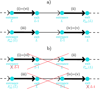
Abbildung 6: a) Encounter stretches (thick lines) and loops (thin lines) of $\gamma^{\prime}$ and $\overline{\gamma^{\prime}}$ in the special case $P_{\rm enc}(\overline{L-1})=L$ and $P_{\rm enc}^{-1}(L-1)=\overline{L}$. The stretches (i) and (vi), and stretches (iv) and (v) of Fig. 5a coincide. In b), the loops $L-1\to L$ and $\overline{L}\to\overline{L-1}$ are removed and entrance $\overline{L}$ and exit $L$ are respectively renamed as entrance $\overline{L-1}$ and exit $L-1$.

To be safe, we need to check that Eq. (29) remains valid in the two special cases $m=l-1$ and $m=1$. First assume that the elements $a_{m+2},\ldots,a_{l}$ and $\overline{a_{l}},\ldots,\overline{a_{m+2}}$ in Eq. (27) are removed, which formally corresponds to $m=l-1$. In this case, Eq. (26) implies $\overline{L-1}=P_{\rm enc}^{l-1}(L)=P_{\rm enc}^{-1}(L)$ and thus $P_{\rm enc}(\overline{L-1})=L$ and $P_{\rm enc}^{-1}(L-1)=\overline{L}$. Our caricature of port connections in Fig. 5a has to be modified, since the stretches (iv) and (v) coincide, as well as (i) and (vi); see Fig. 6a. If we again remove the loops leading from exit $L-1$ to entrance $L$ and from exit $\overline{L}$ to entrance $\overline{L-1}$, rename exit $L$ as $L-1$, and rename entrance $\overline{L}$ as $\overline{L-1}$ (Fig. 6b), we can immediately read off the new encounter permutation

$$Q_{\rm enc}(a)=\begin{cases}L-1&\text{if $a=P_{\rm enc}^{-1}(\overline{L})$}\\ P_{\rm enc}(L)&\text{if $a=\overline{L-1}$}\\ P_{\rm enc}(a)&\text{otherwise}\,.\end{cases}$$ (31)

Our conclusions remain unaffected. The permutation $Q_{\rm enc}$ now differs from $P_{\rm enc}$ by mapping $Q_{\rm enc}(\overline{a_{2}})=L-1$ and $Q_{\rm enc}(\overline{L-1})=a_{2}$. We thus recover Eq. (29), again with $a_{m+2},\ldots,a_{l}$ and $\overline{a_{l}},\ldots,\overline{a_{m+2}}$ removed.

On the other hand, if $a_{2},\ldots,a_{m}$ and $\overline{a_{m}},\ldots,\overline{a_{2}}$ are removed from (27) (corresponding to $m=1$ and $P_{\rm enc}(L)=\overline{L-1}$), the recursion (23) remains in force and implies

$$Q_{\rm enc}(\overline{a_{m+2}}) = \overline{L-1}\,,\quad\quad\quad Q_{\rm enc}(L-1)=a_{m+2}\,,$$

$$Q_{\rm enc}(a_{l}) = L-1\,,\quad\quad\quad Q_{\rm enc}(\overline{L-1})=\overline{a_{l}}\,,$$ (32)

leading to Eq. (29) with the above elements absent. Thus, both special cases were correctly taken into account.

Resulting recursion

We have seen that ${\cal M}(\vec{v},l)$ falls into subsets similar to the unitary case, time-reversal invariance making for the factor 2 explained above, and for $l-1$ additional subsets of size $N(\vec{v}^{[l\to l-1]},l-1)$. The various sizes combine to the orthogonal analog of the recursion relation (11),

$$N(\vec{v},l) = \sum_{k\geq 2}N(\vec{v}^{[k,l\to k+l-1]},k+l-1)$$ (33)

$$+ \sum_{m=1}^{l-2}2(l-m-1)(v_{l-m-1}+1)N(\vec{v}^{[l\to m,l-m-1]},m)$$

$$+ (l-1)N(\vec{v}^{[l\to l-1]},l-1)\,,$$

which using Eq. (2) may be written as

$$\frac{lv_{l}}{L}N(\vec{v}) = \sum_{k\geq 2}\frac{(k+l-1)(v_{k+l-1}+1)}{L-1}N(\vec{v}^{[k,l\to k+l-1]})$$ (34)

$$+ \sum_{m=1}^{l-2}\frac{2(l-m-1)(v_{l-m-1}+1)mv_{m}^{[l\to m,l-m-1]}}{L-1}N(\vec{v}^{[l\to m,l-m-1]})$$

$$+ \frac{(l-1)^{2}(v_{l-1}+1)}{L-1}N(\vec{v}^{[l\to l-1]})\,.$$

The shorthand $\tilde{N}(\vec{v})=N(\vec{v})\frac{(-1)^{V}\prod_{l}l^{v_{l}}}{L}$ leads to

$$v_{l}\tilde{N}(\vec{v})+\sum_{k\geq 2}(v_{k+l-1}+1)k\tilde{N}(\vec{v}^{[k,l\to k+l-1]})$$

$$+\sum_{m=1}^{l-2}2(v_{l-m-1}+1)v_{m}^{[l\to m,l-m-1]}\tilde{N}(\vec{v}^{[l\to m,l-m-1]})$$

$$-(l-1)(v_{l-1}+1)\tilde{N}(\vec{v}^{[l\to l-1]})=0\,;$$ (35)

recall that $v_{k+l-1}+1=v_{k+l-1}^{[k,l\to k+l-1]}$ and $v_{l-1}+1=v_{l-1}^{[l\to l-1]}$.

5 Spectral form factor

Similarly as in Subsection 4 we now turn the recursion relation for $\tilde{N}(\vec{v})$ into one for the Taylor coefficients $K_{n}$. As a preparation we generalize our rule (18). For all similar sums over $\vec{v}$ with fixed $\nu(\vec{v})=n$ and $v_{1}=0$ we find

$$\sum_{\vec{v}}^{\nu(\vec{v})=n}\!\!f(\vec{v}^{[\alpha_{1},\alpha_{2},\ldots\to\beta]})\tilde{N}(\vec{v}^{[\alpha_{1},\alpha_{2},\ldots\to\beta]})=\!\!\!\!\sum_{\vec{v}^{\prime}}^{\nu(\vec{v}^{\prime})=n^{\prime}}\!\!\!f(\vec{v}^{\prime})\tilde{N}(\vec{v}^{\prime})\,,$$ (36)

with integers $\alpha_{i}\geq 2$, $\beta\geq 2$ and $f$ any function of $\vec{v}^{\prime}$ vanishing for $v^{\prime}_{\beta}=0$. We need to sum over all $\vec{v}^{\prime}$ with $n^{\prime}=\nu(\vec{v}^{\prime})=\nu(\vec{v}^{[\alpha_{1},\alpha_{2},\ldots\to\beta]})=n-\sum_{i}(\alpha_{i}-1)+(\beta-1)$, where we used that removing an $\alpha_{i}$-cycle decreases $L$ by $\alpha_{i}$, $V$ by 1, and thus $\nu=L-V+1$ by $\alpha_{i}-1$; similarly, adding a $\beta$-cycle increases $\nu$ by $\beta-1$. Eq. (36) follows in the same way as Eq. (18), i.e., by switching to $\vec{v}^{\prime}=\vec{v}^{[\alpha_{1},\alpha_{2},\ldots\to\beta]}$ as the new summation variable and dropping the restriction $v^{\prime}_{\beta}\geq 1$ ($\vec{v}^{\prime}$ with $v^{\prime}_{\beta}=0$ do not contribute due to the vanishing of $f$). One similarly shows that the foregoing rule holds even without any conditions on $f$ if $\beta$ is removed, i.e., if no new cycles are created. It is convenient to abbreviate the right-hand side of Eq. (36) with the help of

$$S_{n^{\prime}}[f]\equiv\sum_{\vec{v}^{\prime}}^{\nu(\vec{v}^{\prime})=n^{\prime}}f(\vec{v}^{\prime})\tilde{N}(\vec{v}^{\prime})\,$$ (37)

for arbitrary $f$; we note that $K_{n}=\frac{2}{(n-2)!}S_{n}[1]$. Thus equipped we turn to the three special cases $l=1,2,3$ of our recursion relations which we shall need below.

$l=1$

The case $l=1$ involves permutations with 1-cycles, appearing only in intermediate steps of our calculation. If the element $L$ forms a 1-cycle, it may simply be removed from a permutation without affecting the other cycles, which corresponds to a transition $\vec{v}\to\vec{v}^{[1\to]}$. The number of permutations with given $\vec{v}$ and $L$ forming part of a 1-cycle thus coincides with the number of permutations related to $\vec{v}^{[1\to]}$, i.e., $N(\vec{v},1)=N(\vec{v}^{[1\to]})$ and equivalently

$$\tilde{N}(\vec{v})=-\frac{L(\vec{v}^{[1\to]})}{v_{1}}\tilde{N}(\vec{v}^{[1\to]})\,.$$ (38)

$l=2$

For $l=2$ (and $v_{1}=0$) the recursion (4) boils down to

$$v_{2}\tilde{N}(\vec{v})+\sum_{k\geq 2}\left(v_{k+1}^{[k,2\to k+1])}k\tilde{N}(\vec{v}^{[k,2\to k+1]})\right)-\tilde{N}(\vec{v}^{[2\to 1]})=0\,,$$ (39)

where only the last term is new compared to the unitary case; to determine its prefactor we have used that $(l-1)(v_{l-1}+1)=1$ for $l=2$, $v_{1}=0$. We can bring this term to a form free from 1-cycles by invoking Eq. (38) and thus $\tilde{N}(\vec{v}^{[2\to 1]})=-L(\vec{v}^{[2\to]})\tilde{N}(\vec{v}^{[2\to]})$, to get

$$v_{2}\tilde{N}(\vec{v})+\sum_{k\geq 2}\left(v_{k+1}^{[k,2\to k+1])}k\tilde{N}(\vec{v}^{[k,2\to k+1]})\right)+L(\vec{v}^{[2\to]})\tilde{N}(\vec{v}^{[2\to]})=0\,.$$ (40)

Again, we sum over all $\vec{v}$ with $v_{1}=0$ and $\nu(\vec{v})=n$. The sum over the first two terms of (40) may be evaluated as in the unitary case. Using the rule (36) and the shorthand (37), the sum over the third term leads to

$$\sum_{\vec{v}}^{\nu(\vec{v})=n}L(\vec{v}^{[2\to]})\tilde{N}(\vec{v}^{[2\to]})=S_{n-1}[L(\vec{v})]$$ (41)

where we used that removal of a 2-cycle decreases $\nu$ by 1. Altogether, we obtain

$$S_{n}\Bigg{[}v_{2}+\sum_{k\geq 2}v_{k+1}k\Bigg{]}+S_{n-1}[L(\vec{v})]$$

$$=(n-1)S_{n}[1]+S_{n-1}[L(\vec{v})]=0\,.$$ (42)

A further relation is obtained by multiplying Eq. (40) with $L(\vec{v})-1=L(\vec{v}^{[k,2\to k+1]})=L(\vec{v}^{[2\to]})+1$,

$$(L(\vec{v})-1)v_{2}\tilde{N}(\vec{v})+\sum_{k\geq 2}\left(L(\vec{v}^{[k,2\to k+1]})v_{k+1}^{[k,2\to k+1])}k\tilde{N}(\vec{v}^{[k,2\to k+1]})\right)$$

$$+L(\vec{v}^{[2\to]})(L(\vec{v}^{[2\to]})+1)\tilde{N}(\vec{v}^{[2\to]})=0\,.$$ (43)

Summing over $\vec{v}$ with the help of (36) and (37), we obtain

$$S_{n}\Bigg{[}(L(\vec{v})-1)v_{2}+\sum_{k\geq 2}L(\vec{v})v_{k+1}k\Bigg{]}+S_{n-1}[L(\vec{v})(L(\vec{v})+1)]=0$$ (44)

and thus

$$(n-1)S_{n}[L(\vec{v})]-S_{n}[v_{2}]+S_{n-1}[L(\vec{v})(L(\vec{v})+1)]=0\,.$$ (45)

This equation can be simplified if we eliminate $S_{n}[L(\vec{v})]$ with the help of Eq. (5) and replace $n\to n-2$,

$$-(n-2)(n-3)S_{n-1}[1]=S_{n-2}[v_{2}]-S_{n-3}[L(\vec{v})(L(\vec{v})+1)]\,.$$ (46)

$l=3$

Finally, we consider the special case $l=3$ (and $v_{1}=0$) of (4),

$$v_{3}\tilde{N}(\vec{v})+\sum_{k\geq 2}\left(v_{k+2}^{[k,3\to k+2]}k\tilde{N}(\vec{v}^{[k,3\to k+2]})\right)$$

$$+4\tilde{N}(\vec{v}^{[3\to 1,1]})-2v_{2}^{[3\to 2]}\tilde{N}(\vec{v}^{[3\to 2]})=0\,.$$ (47)

The third term originates from the sum over $m$ in (4) which only draws a contribution from $m=1$, with the prefactor $2(v_{1}+1)v_{1}^{[3\to 1,1]}=4$. The 1-cycles are eliminated using the identity $\tilde{N}(\vec{v}^{[3\to 1,1]})=\frac{1}{2}L(\vec{v}^{[3\to]})(L(\vec{v}^{[3\to]})+1)\tilde{N}(\vec{v}^{[3\to]})$, which follows by twice applying Eq. (38) to $\vec{v}^{[3\to 1,1]}$. We thus find

$$v_{3}\tilde{N}(\vec{v})+\sum_{k\geq 2}\left(v_{k+2}^{[k,3\to k+2]}k\tilde{N}(\vec{v}^{[k,3\to k+2]})\right)$$

$$+2L(\vec{v}^{[3\to]})(L(\vec{v}^{[3\to]})+1)\tilde{N}(\vec{v}^{[3\to]})-2v_{2}^{[3\to 2]}\tilde{N}(\vec{v}^{[3\to 2]})=0\,.$$ (48)

It is easy to see that Eq. (5) connects combinatorial numbers related to three different orders of $K(\tau)$. If $\vec{v}$ and thus $\vec{v}^{[k,3\to k+2]}$ contribute to order $n$, $\vec{v}^{[3\to]}$ contributes to $n-2$, and $\vec{v}^{[3\to 2]}$ contributes to $n-1$. Summing over $\vec{v}$, we find

$$S_{n}\Bigg{[}v_{3}+\sum_{k\geq 2}v_{k+2}k\Bigg{]}+2S_{n-2}[L(\vec{v})(L(\vec{v})+1)]-2S_{n-1}[v_{2}]=0\,.$$ (49)

This expression can be simplified using that $v_{3}+\sum_{k\geq 2}v_{k+2}k=\sum_{l\geq 2}v_{l}(l-2)=L(\vec{v})-2V(\vec{v})=2(\nu(\vec{v})-1)-L(\vec{v})$, which leads to

$$2(n-1)S_{n}[1]-S_{n}[L(\vec{v})]+2S_{n-2}[L(\vec{v})(L(\vec{v})+1)]-2S_{n-1}[v_{2}]=0\,.$$ (50)

Finally applying Eq. (5) to eliminate $S_{n}[L(\vec{v})]$, substituting $n\to n-1$, and dividing by 2, we proceed to

$$\frac{n-1}{2}S_{n}[1]+(n-2)S_{n-1}[1]=S_{n-2}[v_{2}]-S_{n-3}[L(\vec{v})(L(\vec{v})+1)]\,.$$ (51)

Final result

Upon comparing the recursion relations (46) and (51), obtained for the cases $l=2$ and $l=3$, we find the coefficients $S_{n}[1]=\frac{(n-2)!}{2}K_{n}$ and $S_{n-1}[1]=\frac{(n-3)!}{2}K_{n-1}$ related as $\frac{n-1}{2}S_{n}[1]=-(n-2)^{2}S_{n-1}[1]$ or

$$(n-1)K_{n}=-2(n-2)K_{n-1}\,.$$ (52)

Eq. (52) applies to all $n\geq 3$, but not to $n=2$, because the diagonal term $K_{1}$ is unrelated to our permutation treatment.

An initial condition is provided by the Sieber/Richter result for orbits differing in one 2-encounter, $K_{2}=-2$. Thus started, our recursion yields the Taylor coefficients

$$K_{n}=\frac{(-2)^{n-1}}{n-1}$$ (53)

coinciding with the random-matrix result from the GOE. Universal behavior is thus ascertained for the small-time form factor of fully chaotic dynamics from the orthogonal symmetry class, at least in the limit $\tau\ll 1$. The resulting series converges for $\tau<\frac{1}{2}$ and remains valid, by analytic continuation, up to the singularity at $\tau=1$.

3 Summary

We have shown that structures of orbit pairs $\gamma$, $\gamma^{\prime}$ are in one-to-one correspondence to permutations. Encounters are described by permutations $P_{\rm enc}$ determining how the ports of $\gamma$ are reconnected in $\gamma^{\prime}$, i.e., which entrance port is connected to which exit port. In absence of time-reversal invariance, $P_{\rm enc}$ has one cycle per encounter. Loops are characterized by another permutation $P_{\rm loop}$ fixing the entrance port following each exit port. The ordering of entrance ports along $\gamma^{\prime}$ is thus given by the product $P_{\rm loop}P_{\rm enc}$ which must be single-cycle due to the periodicity of $\gamma^{\prime}$.

For time-reversal invariant systems, we consider permutations mapping between ports of both $\gamma$ and its time reversed $\overline{\gamma}$. In this case encounters correspond to pairs of “mutually time-reversed” cycles, and $P_{\rm loop}P_{\rm enc}$ has one cycle related to $\gamma^{\prime}$ and one cycle related to $\overline{\gamma^{\prime}}$.

The numbers of structures $N(\vec{v})$ can now be determined from a recursion, motivated by the physical picture of “removing loops” between encounters. This recursion translates into a recursion for the Taylor coefficients of $K(\tau)$ which indeed yields small-time form factors in agreement with the GUE and the GOE.

Kapitel 6 Relation to the $\sigma$ model

1 Introduction

The so-called nonlinear $\sigma$ model [47, 48] is a convenient framework for calculating spectral correlators or, more generally, averaged products of Green functions. In particular, the zero-dimensional variant of the $\sigma$ model can be used to implement averages over random matrices of the Wigner/Dyson ensembles, as required to evaluate the corresponding spectral form factors $K(\tau)$. Similarly, for disordered systems, the $\sigma$ model has been used to implement averages over impurity potentials. Steps towards a ballistic $\sigma$ model for individual systems have been presented in [8].

The $\sigma$ model proved of great heuristic value for our semiclassical approach: We were led to the correct combinatorics of families of orbit pairs by a perturbative analysis of the $\sigma$ model. Such a perturbative treatment yields the spectral form factor as power series in the time $\tau$, analogous the series extracted from Gutzwiller’s semiclassical periodic-orbit theory in the preceding Chapters. In order to gain intuition for our semiclassical analysis, the perturbative treatment of the $\sigma$ model had to be carried to all orders in $\tau$. To our knowledge, this task has never been attacked explicitly before, since within random-matrix theory the whole spectral form factor is accessible through a non-perturbative approach. The analogy of periodic-orbit expansions to perturbation series might prove fruitful for future applications of periodic-orbit theory, and that possibility motivates the following exposition.

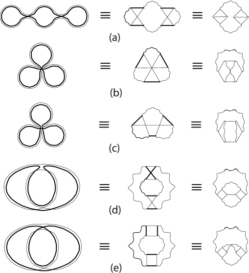
Abbildung 1: Families of orbit pairs (left column) and the corresponding disorder diagrams (middle and right column), responsible for the cubic order of $K(\tau)$. The Figure is taken from [10]. The cases (a)-(e) respectively correspond to the families aas, pc, ac, api, and ppi discussed in Chapter 3. (There are slight inconsistencies in the cases (d) and (e).) In the middle column, diagrams are arranged such as to stress the analogy to orbits; the right column follows usual field-theoretical conventions.

We will mostly work with the $\sigma$ model in a random-matrix setting. However, it will be worthwhile to at least qualitatively point out similarities to the diagrammatic expansion yielding $K(\tau)$ for disordered systems. These similarities were first noticed in [10, 11], in a previous attempt to recover the form factor for individual chaotic dynamics. Fig. 1, taken from [10], displays the diagrams responsible for the cubic contribution to the form factor. We see that these diagrams are in one-to-one correspondence to the families of orbit pairs discussed in Chapter 3 and depicted, in a slightly different style, in the left column. The shapes drawn by straight lines are known as “Hikami boxes”; these boxes form a particular kind of vertex. Hikami boxes are analogous to self-encounters of periodic orbits, with each $l$-encounter leading to a Hikami box with $2l$ “ports” depicted as corners. The straight lines correspond to encounter stretches of the two partner orbits; the thick and thin straight lines in the middle column of Fig. 1 can respectively be associated with stretches of the partner orbits drawn in the left column. The Hikami boxes related to parallel and antiparallel 2-encounters are known as diffusons and Cooperons. (In contrast to the interpretation in terms of classical orbits, in field theory diffusons are often depicted by antiparallel arrows, whereas Cooperons are denoted by parallel arrows.) Outside the Hikami boxes, the ports are connected by (curly) propagator lines – obviously the analog of orbit loops. Each diagram should be taken to represent all possible orbit pairs obtainable by reconnections in encounters of the same topology as the Hikami boxes depicted.

In field theory, vertices are essentially points (even though they are depicted in a different manner in Fig. 1) – in contrast to periodic-orbit theory where the related encounters have a non-zero duration, of the order of the Ehrenfest time $T_{E}\propto\ln\frac{\rm const}{\hbar}$. Of course, the relevant encounter durations are vanishingly small compared to the typical loop durations ($\sim T_{H}\propto\hbar^{-f+1}$); nevertheless, we may say that self-encounters give internal (phase-space) structure to vertices.

In the remainder of this Chapter, the relation between periodic-orbit theory and the $\sigma$ model will be explored from a random-matrix perspective. We shall first introduce the bosonic replica variant of the zero-dimensional nonlinear $\sigma$ model. In Subsection 3, the resulting spectral form factor $K(\tau)$ will be expanded perturbatively into a sum over vectors $\vec{v}$, analogous to the sum obtained from periodic-orbit theory. Wick’s theorem can be used to recursively evaluate each summand, with the help of contraction rules introduced in Subsections 1 and 2. These contraction rules have a striking similarity to semiclassics: In Subsection 3 we will reveal both expansions for $K(\tau)$ as identical, by relating structures of orbit pairs to so-called “full contractions” in the $\sigma$ model. In Subsection 4 we shall see that the recursion for the numbers of structures $N(\vec{v})$ in Chapter 5 is mirrored by an analogous recursion based on Wick contractions in the $\sigma$ model.

2 Background: The nonlinear $\sigma$ model

We proceed to give a brief introduction to the nonlinear $\sigma$ model, in a random-matrix setting. In particular, we will show that the bosonic replica variant of the $\sigma$ model yields the $\frac{1}{s}$-expansion of the two-point correlator

$$R(s)=\left\langle\frac{\rho(E+\frac{s}{2\pi\overline{\rho}})\rho(E-\frac{s}{2\pi\overline{\rho}})}{\overline{\rho}(E)^{2}}\right\rangle-1\,,$$ (1)

see also Eq. (19), as an integral over matrices $B$,

$$R(s)\sim-\frac{1}{2}{\rm Re}\ {\rm lim}_{r\to 0}\frac{1}{r^{2}}\partial^{2}_{s^{+}}\,{(s^{+})}^{-\kappa r^{2}}{\rm e}^{is^{+}r}\int{d[B]}\,{\rm e}^{(2{{\rm i}}/\kappa)\sum_{l=1}^{\infty}{(s^{+})}^{1-l}{\rm tr}(B{B^{\dagger}})^{l}}-\frac{1}{2}\,;$$ (2)

an analogous formula for $K(\tau)$ is obtained by Fourier transforming according to (20). On the right-hand side, $s^{+}$ must be read as $s+{{\rm i}}\delta^{\prime}$ with $\delta^{\prime}\downarrow 0$. The matrices $B,{B^{\dagger}}$ are $r\times r$ for the GUE and $2r\times 2r$ for the GOE, and the measure $d[B]$ will be defined in Eq. (26); as before, the factor $\kappa$ takes the respective values 1 and 2 for the unitary and the orthogonal cases. The above formula yields only the non-oscillatory part of $R(s)$, needed to recover the power series of $K(\tau)$; the dropping of oscillatory terms is signaled by $\sim$. Eq. (2) will later serve as the starting point for our perturbative treatment of the spectral form factor, paralleling the previous semiclassical approach.

1 Average over the GUE

To derive the random-matrix expression for the two-point correlator (2), we first consider the GUE. The average $\langle\ldots\rangle$ over small intervals of $E$ and $s$ in (1) is thus replaced by an average $\overline{\rule{0.0pt}{5.8125pt}\ldots\rule{0.0pt}{5.8125pt}}$ over all independent matrix elements $H_{\mu\nu}$ of Hermitian $N\times N$ matrices, with $N\to\infty$ and a Gaussian weight defined by

$$\overline{\rule{0.0pt}{5.8125pt}\ldots\rule{0.0pt}{5.8125pt}}\equiv\int d[H]\;{\cal A}\,{\rm e}^{-{\cal B}{\rm Tr}H^{2}}\ldots\equiv\int\prod_{\mu<\nu}(d\mbox{Re}H_{\mu\nu}\,d\mbox{Im}H_{\mu\nu})\prod_{\mu}dH_{\mu\mu}\;{\cal A}\,{\rm e}^{-{\cal B}{\rm Tr}H^{2}}\ldots\,$$ (3)

We choose ${\cal A}$ and ${\cal B}$ such that the Gaussian weight is normalized and, moreover, the average of each squared matrix element is given by $\overline{|H_{\mu\nu}|^{2}}=\frac{\lambda^{2}}{N}$ with $\lambda$ constant. In particular, this choice implies ${\cal B}=\frac{N}{2\lambda^{2}}$. All other products of matrix elements $H_{\mu\nu}H^{*}_{\mu^{\prime}\nu^{\prime}}$, $(\mu,\nu)\neq(\mu^{\prime},\nu^{\prime})$ have to average to zero regardless of ${\cal A}$ and ${\cal B}$. In the following, we shall always consider the vicinity of $E=0$, where the average level density is given by $\overline{\rho}=\frac{N}{\pi\lambda}$.

Green functions

It is convenient to express $\rho(E)$ and $R(s)$ in terms of the advanced and retarded Green functions

$$G_{\pm}(E)=(E\pm{{\rm i}}\delta-H)^{-1}\,,$$ (4)

where we implicitly take $\delta\downarrow 0$. Writing the diagonal elements of $G_{\pm}(E)$ as

$$\frac{1}{(E-E_{n})\pm{{\rm i}}\delta}=P\frac{1}{E-E_{n}}\mp{{\rm i}}\pi\delta(E-E_{n})\,$$ (5)

with $P$ denoting the principal value, one can show that the level density is simply given by

$$\rho(E)=\frac{{\rm i}}{2\pi}({\rm Tr}\,G_{+}(E)-{\rm Tr}\,G_{-}(E))\,.$$ (6)

Eqs. (1), (3), and (6) entail the corresponding expression for the correlator

$$R(s) = \frac{1}{2(\pi\overline{\rho})^{2}}\mbox{Re}\,C(s)-\frac{1}{2}$$ (7)

with $C(s)$ defined by

$$C(s) \equiv \overline{{\rm Tr}\,G_{+}\left(E+\frac{s}{2\pi\overline{\rho}}\right){\rm Tr}\,G_{-}\left(E-\frac{s}{2\pi\overline{\rho}}\right)}\,.$$ (8)

Generating function

Rather than expressing $R(s)$ through traces of $G_{\pm}(E)$, it is technically simpler to work with determinants. To translate between the two, we use the “replica trick”: For $r$ real and $f(E)\equiv\det G_{\pm}(E)^{-1}$, we have

$${\rm tr}\,G_{\pm}(E) = \partial_{E}{\,\rm Tr}\ln(E\pm{{\rm i}}\delta-H)=\partial_{E}{\,\rm Tr}\ln(G_{\pm}(E)^{-1})$$ (9)

$$= \partial_{E}\ln f(E)=\frac{f^{\prime}(E)}{f(E)}=\lim_{r\to 0}f(E)^{-r-1}f^{\prime}(E)$$

$$= -\lim_{r\to 0}\frac{1}{r}\partial_{E}f(E)^{-r}=-\lim_{r\to 0}{1\over r}\partial_{E}\det G_{\pm}(E)^{r}\,.$$

As usual, we assume (9) valid even if the so-called replica index $r$ is restricted to the integer numbers. This assumption obviously demands mathematical justification, which is beyond the scope of this thesis.

Invoking the replica trick for both traces in (8), we represent $C(s)$ as the two-fold derivative of a generating function ${\cal Z}(\epsilon_{+},\epsilon_{-})$ involving determinants of Green functions,

$$C(s) = \lim_{r\to 0}\frac{1}{r^{2}}\left[\frac{\partial^{2}{\cal Z}(\epsilon_{+},\epsilon_{-})}{\partial\epsilon_{+}\partial\epsilon_{-}}\right]_{\epsilon_{\pm}=\pm\frac{\epsilon}{2}=\pm\frac{s}{2\pi\overline{\rho}}}$$

$${\cal Z}(\epsilon_{+},\epsilon_{-}) = \overline{\det G_{-}(E+\epsilon_{+})^{r}\det G_{+}(E+\epsilon_{-})^{r}}\,.$$ (10)

Crucially, such determinants allow for the integral representation

$$\det{G}_{\pm}=\int d[\phi]\exp\left(\pm{{\rm i}}\phi^{\dagger}G_{\pm}^{-1}\phi\right)$$ (11)

where the integration runs over $N$-dimensional complex vectors $\phi$ with the measure defined by $d[\phi]=\prod_{\mu=1}^{N}\frac{d{\rm Re}\phi\,d{\rm Im}\phi}{\pi}$. The sign in the exponent of (11) is chosen such as to make the integral convergent. The individual determinants in Eq. (1) can now be numbered by $\alpha=1,\ldots,2r$ (with $\alpha=1,\ldots,r$ corresponding to the advanced and $\alpha=(r+1),\ldots,2r$ to the retarded Green functions), and each represented as an integral

$$\det G_{\pm}(E+\epsilon_{\pm})=\int d[\psi^{\alpha}]\,\exp\left(\pm{{\rm i}}\psi^{\alpha\dagger}(E+(\epsilon_{\pm}\pm{{\rm i}}\delta)-H)\psi^{\alpha}\right)\,;$$ (12)

over $\psi^{\alpha}=\{\psi^{\alpha}_{\mu}\}$, $\mu=1,\ldots,N$.

All $2r$ integrals together may be written as

$${\cal Z}(\epsilon_{+},\epsilon_{-}) = \overline{\int d[\psi]\exp\Big{(}{{\rm i}}\sum_{\alpha=1,\ldots,2r}{\psi^{\alpha}}^{\dagger}\Lambda^{\alpha}(E+\hat{\epsilon}^{\alpha}-H)\psi^{\alpha}\Big{)}}$$ (13)

with

$$d[\psi] = \prod_{\alpha=1}^{2r}d[\psi^{\alpha}]$$

$$\Lambda^{\alpha} = \begin{cases}1&\mbox{for $\alpha=1,\ldots,r$}\\ -1&\mbox{for $\alpha=(r+1),\ldots,2r$}\end{cases}$$

$$\hat{\epsilon}^{\alpha} = \begin{cases}\epsilon_{+}+{{\rm i}}\delta&\mbox{for $\alpha=1,\ldots,r$}\\ \epsilon_{-}-{{\rm i}}\delta&\mbox{for $\alpha=(r+1),\ldots,2r$\;.}\end{cases}$$ (14)

In the following, we will drop the index $\alpha$, and simply write

$${\cal Z}(\epsilon_{+},\epsilon_{-})=\overline{\int d[\psi]\exp\left({{\rm i}}\psi^{\dagger}\Lambda(E+\hat{\epsilon}-H)\psi\right)}\,.$$ (15)

The resulting $H$ now has to be read as a block-diagonal matrix with $2r$ identical $N\times N$ blocks containing the matrix elements of the Hamiltonian. $\Lambda$ and $\hat{\epsilon}$ turn into diagonal matrices with diagonal elements given by (1), i.e., $\Lambda=\operatorname{diag}({\mathbf{1}}_{rN},-{\mathbf{1}}_{rN})$, $\hat{\epsilon}=\operatorname{diag}((\epsilon_{+}+{{\rm i}}\delta){\mathbf{1}}_{rN},(\epsilon_{-}-{{\rm i}}\delta){\mathbf{1}}_{rN})$, where ${\mathbf{1}}_{rN}$ is the $rN$-dimensional unit matrix. (Analogous $2r\times 2r$ matrices will later be denoted by the same symbols $\Lambda$, $\hat{\epsilon}$.)

Average over $H$ for fixed $\psi$

The replica representation (15) has an important advantage: If we exchange the $\psi$ integration and the average over $H$ implied by $\overline{\rule{0.0pt}{5.8125pt}\ldots\rule{0.0pt}{5.8125pt}}$, we obtain a simple Gaussian integral

$${\cal Z}(\epsilon_{+},\epsilon_{-})=\int d[\psi]\exp({{\rm i}}\psi^{\dagger}\Lambda(E+\hat{\epsilon})\psi)\int d[H]{\cal A}\exp\left(-\frac{N}{2\lambda^{2}}{\rm Tr}H^{2}-{{\rm i}}\psi^{\dagger}\Lambda H\psi\right)\,.$$ (16)

To evaluate this integral, for fixed $\psi$, we first need eliminate to the term linear in $H$. This can be achieved by writing $-{{\rm i}}\psi^{\dagger}\Lambda H\psi=-{{\rm i}}{\rm Tr}\,HX$ with $X_{\mu\nu}=\sum_{\alpha}{\psi_{\nu}^{\alpha}}^{*}\Lambda^{\alpha}\psi_{\mu}^{\alpha}$ (or, in short, $X_{\mu\nu}={\psi_{\nu}}^{\dagger}\Lambda\psi_{\mu}$) and transforming $H+\frac{{{\rm i}}\lambda^{2}}{N}X\to H$. Through this transformation, the exponent obtains a new summand $-\frac{\lambda^{2}}{2N}{\rm Tr}\,X^{2}=-\frac{\lambda^{2}}{2N}{\,\rm tr\,}A^{2}$, where ${\,\rm tr\,}$ denotes a trace over $\alpha$, and $A^{\alpha\beta}=\sum_{\mu}\psi_{\mu}^{\alpha}{\psi_{\mu}^{\beta}}^{*}\Lambda^{\beta}$. The remaining Gaussian integral $\int d[H]{\cal A}\exp\left(-\frac{N}{2\lambda^{2}}{\,\rm tr\,}H^{2}\right)$ gives unity, due to the normalization of the Gaussian weight. We thus find

$${\cal Z}(\epsilon_{+},\epsilon_{-})=\int d[\psi]\exp\left({\rm i}\psi^{\dagger}\Lambda(\hat{\epsilon}+E)\psi-\frac{\lambda^{2}}{2N}{\rm tr\,}A^{2}\right)\,.$$ (17)

Hubbard–Stratonovich transformation

To proceed, we need to eliminate the term $\propto{\rm tr}\,A^{2}$ quartic in the integration variables $\psi$ by a so-called Hubbard–Stratonovich transformation. To this end, we again introduce an additional integration, and multiply $\mathcal{Z}$ by a Gaussian integral $\int d[Q]\,\exp\left(\frac{N}{2}{\rm tr}\,Q^{2}\right)$, where $Q=\{Q^{\alpha\beta}\}$ is a $2r$–dimensional anti-Hermitian matrix and $\int d[Q]$ denotes integration over all its independent matrix elements. That integral is convergent, since the exponent may be written as $-\frac{N}{2}{\,\rm tr\,}({{\rm i}}Q)^{2}$ with ${{\rm i}}Q$ Hermitian, and yields an $r$-fold power, going to 1 in the replica limit $r\to 0$. Denoting equivalence in the replica limit by $\sim$ and transforming $Q\to Q-\lambda A/N$, we are led to

$$\mathcal{Z}(\epsilon_{+},\epsilon_{-})\!\! \sim \!\!\!\!\!\int\!\!d[Q]\!\int\!\!d[\psi]\exp\!\left({\textstyle{\frac{N}{2}}}{\rm tr}\,Q^{2}+{\rm i}\psi^{\dagger}\Lambda(\hat{\epsilon}+E+{\rm i}\lambda Q)\psi\right)\,,$$ (18)

with the quartic term removed.

The $\psi$ integral has now become easy: Each of the $N$ independent Gaussian integrations over $\psi_{\mu}=\{\psi_{\mu}^{\alpha}\}$ yields a determinant that can be incorporated into the exponent via “$\det=\exp{\,\rm tr\,}\ln$”, to get

$$\mathcal{Z}(\epsilon_{+},\epsilon_{-}) \sim \!\!\!\!\int\!\!d[Q]\,\exp\left({\textstyle{\frac{N}{2}}}{\rm tr}\,Q^{2}-N{\rm\,tr\,ln}(\hat{\epsilon}+E+{\rm i}\lambda Q)\right)\;\;\;\;\;\;\,$$ (19)

$$= \!\!\!\!\int\!\!d[Q]\,\exp\left(-N{\rm\,tr\,ln}\left(1+\frac{\hat{\epsilon}}{E+{\rm i}\lambda Q}\right)\right)$$

$$\;\;\;\;\;\times\exp\left(N\left\{\frac{1}{2}{\rm tr}\,Q^{2}-{{\,\rm tr\,}\,\ln}(E+{\rm i}\lambda Q)\right\}\right)\,.\;\;\;\;\;\;$$

The generating function is thus expressed as an integral in replica space. The only reminder left of the original matrices $H$ is their dimension $N$.

Saddle-point approximation

The integral over $Q$ has to be evaluated in the limit of infinite matrix dimension $N\to\infty$. Since $\hat{\epsilon}$ is of the order of the mean level spacing and thus proportional to $\frac{1}{N}$, the exponential in the second line of Eq. (19), the so-called “amplitude”, may be approximated as $\exp(-{\,\rm tr\,}\frac{N\hat{\epsilon}}{E+{\rm i}\lambda Q})$ by expanding the logarithm.

In the following exponential, the large parameter $N\to\infty$ is not compensated by a factor $\hat{\epsilon}$. Thus, a saddle-point approximation is called for. The remainder of the exponent, the “action” $S(Q)\equiv\frac{1}{2}{\rm tr}\,Q^{2}-{{\,\rm tr\,}\,\ln}(E+{\rm i}\lambda Q)$, becomes stationary for

$$Q=\frac{{\rm i}\lambda}{E+{\rm i}\lambda Q}\,,$$ (20)

i.e., $Q=Q^{-1}$ if we restrict ourselves to $E=0$. This condition is satisfied by all diagonal matrices with entries $\pm 1$. Among these, one can show that only the saddle point $\Lambda=\mbox{diag}({\mathbf{1}}_{r},-{\mathbf{1}}_{r})$ is relevant for the short-time form factor [49].

The restriction $Q=Q^{-1}$ is also fulfilled by all matrices $Q_{\rm s}=T\Lambda T^{-1}$ similar to $\Lambda$. To make the subsequent integrals convergent we have to restrict ourselves to pseudounitary transformation matrices $T\in U(r,r)$, $T\Lambda T^{\dagger}=\Lambda$ [50]. Several $T$ lead to the same $Q_{\rm s}$: Since transformations from $U(r)\times U(r)$ commute with $\Lambda$, $T$ may be multiplied with any such transformation without affecting the saddle point $Q_{\rm s}$. The saddle-point manifold of all possible $Q_{\rm s}$ can thus be identified with the set of equivalence classes of possible $T$, denoted by ${\rm U}(r,r)/({\rm U}(r)\times{\rm U}(r))$. (This set can be interpreted as a so-called “symmetric space”, see [50].)

To evaluate (18), we have to expand the action to quadratic order in the deviation $Q-Q_{\rm s}$ from the saddle-point manifold, and split integration into one integral over the points $Q_{\rm s}$ on the saddle-point manifold, and one integral over the deviations $Q-Q_{\rm s}$. Approximating the amplitude by its value at the saddle point $Q_{\rm s}$, we then find (in somewhat sloppy notation)

$$\mathcal{Z}(\epsilon_{+},\epsilon_{-}) \sim \int d[Q_{\rm s}]\,\exp\left(-{{\,\rm tr\,}\,}\frac{N\hat{\epsilon}}{E+{\rm i}\lambda Q_{\rm s}}\right)$$ (21)

$$\times\int d[Q-Q_{\rm s}]\exp\left(N\Big{\{}S(Q_{\rm s})+\frac{1}{2}S^{\prime\prime}(Q_{\rm s})(Q-Q_{\rm s})^{2}\Big{\}}\right)\,.$$

The integral over $Q-Q_{\rm s}$ (also including the stationary value of the action) leads, once more, to an $r$-fold power, converging to 1 in the limit $r\to 0$. We are thus left with an integral over the saddle-point manifold involving only the amplitude $\exp(-{\,\rm tr\,}\frac{N\hat{\epsilon}}{E+{\rm i}\lambda Q_{\rm s}})$,

$$\mathcal{Z}(\epsilon_{+},\epsilon_{-}) \sim \int d[Q_{\rm s}]\exp\left(-{\,\rm tr\,}\frac{N\hat{\epsilon}}{E+{\rm i}\lambda Q_{\rm s}}\right)\,.$$ (22)

The latter amplitude can be simplified if we use (20) and, furthermore, decompose the $2r\times 2r$ matrices $\hat{\epsilon}$ and $\Lambda$ into blocks of size $r\times r$, as in

$$-{\,\rm tr\,}\frac{N\hat{\epsilon}}{E+{\rm i}\lambda Q_{\rm s}} \stackrel{{\scriptstyle(\ref{saddle})}}{{=}} \frac{{\rm i}N}{\lambda}{\,\rm tr\,}\hat{\epsilon}\,Q_{\rm s}$$ (23)

$$= \frac{{\rm i}N}{\lambda}{\,\rm tr\,}\Big{(}{\epsilon_{+}+{\rm i}\delta\atop 0}{0\atop\epsilon_{-}-{\rm i}\delta}\Big{)}\Big{(}{Q_{{\rm s},11}\atop{*}}{{*}\atop Q_{{\rm s},22}}\Big{)}$$

$$= \frac{{\rm i}N}{\lambda}{\,\rm tr\,}\Big{(}{(\epsilon_{+}+{\rm i}\delta)Q_{{\rm s},11}\atop{*}}{{*}\atop(\epsilon_{-}-{\rm i}\delta)Q_{{\rm s},22}}\Big{)}$$

$$= \frac{{\rm i}N}{\lambda}\left((\epsilon_{+}+{\rm i}\delta){\,\rm tr\,}Q_{{\rm s},11}+(\epsilon_{-}-{\rm i}\delta){\,\rm tr\,}Q_{{\rm s},22}\right)$$

$$= \frac{{\rm i}N}{2\lambda}\Big{(}(\epsilon_{+}+\epsilon_{-})({\,\rm tr\,}Q_{{\rm s},11}+{\,\rm tr\,}Q_{{\rm s},22})$$

$$\;\;\;\;\;\;\;+(\epsilon_{+}-\epsilon_{-}+2{\rm i}\delta)({\,\rm tr\,}Q_{{\rm s},11}-{\,\rm tr\,}Q_{{\rm s},22})\Big{)}$$

$$= \frac{{\rm i}s^{+}}{2}{\,\rm tr\,}\Lambda Q_{\rm s}\,.$$

In the last step, we used that ${\,\rm tr\,}Q_{{\rm s},11}+{\,\rm tr\,}Q_{{\rm s},22}={\,\rm tr\,}Q_{\rm s}={\,\rm tr\,}(T\Lambda T^{-1})={\,\rm tr\,}\Lambda=0$ and substituted $s^{+}\equiv(\epsilon_{+}-\epsilon_{-}+2{\rm i}\delta)\pi\overline{\rho}=(\epsilon_{+}-\epsilon_{-}+2{\rm i}\delta)\frac{N}{\lambda}$. Altogether, we thus obtain

$$\mathcal{Z}(\epsilon_{+},\epsilon_{-}) \sim \int d[Q_{\rm s}]\,\exp{\left(\frac{{\rm i}s^{+}}{2}{\rm tr}\Lambda Q_{\rm s}\right)}\,.$$ (24)

Rational parametrization

The integral (24) over the saddle-point manifold can be performed if we parametrize $Q_{\rm s}$ by $r\times r$ matrices $B$ as

$$Q_{\rm s}=(1-W)\Lambda(1-W)^{-1}\,;\;\;\;\;\;W=\frac{1}{\sqrt{s^{+}}}\left({0\atop B^{\dagger}}{B\atop 0}\right)\,,$$ (25)

where the scaling factor $\frac{1}{\sqrt{s^{+}}}$ makes for notational convenience. The matrices $1-W$ are proportional to the pseudounitary transformations $T$ mentioned above; the ($B$-dependent) prefactor cancels in (25). In this so-called rational parametrization, the measure $d[Q_{\rm s}]$ may be written as

$$d[Q_{\rm s}]\sim(s^{+})^{-r^{2}}d[B]\equiv(s^{+})^{-r^{2}}\prod_{i,j=1,\ldots,r}(d{\rm Re}B_{ij}\,d{\rm Im}B_{ij})$$ (26)

The exponent appearing in the generating function (24) can be parametrized by inserting (25) and expanding as in $(1-W)^{-1}=\sum_{n=0}^{\infty}W^{n}$. We then find ${\,\rm tr\,}\Lambda Q_{\rm s}=2r+4\sum_{l=1}^{\infty}(s^{+})^{-l}{\,\rm tr\,}(BB^{\dagger})^{l}$, and the whole generating function is expressed as

$$\mathcal{Z}(\epsilon_{+},\epsilon_{-})\sim(s^{+})^{-\kappa r^{2}}\,{\rm e}^{{\rm i}s^{+}r}\int{d[B]}\,{\rm e}^{(2{{\rm i}}/\kappa)\sum_{l=1}^{\infty}(s^{+})^{1-l}{\rm tr}(B{B^{\dagger}})^{l}}\,,$$ (27)

where the factor $\kappa=1$ has been sneaked in for later use.

Using Eqs. (7), (1), and (27), it is easy to check that the resulting two-point correlator $R(s)$ is indeed of the form (2). We only have to realize that, when applied to functions of $s^{+}=(\epsilon_{+}-\epsilon_{-}+2{\rm i}\delta)\pi\overline{\rho}$, the double derivative $\frac{\partial^{2}}{\partial\epsilon_{+}\partial\epsilon_{-}}$ of (1) acts like $-\pi^{2}\overline{\rho}^{2}\frac{\partial^{2}}{\partial{s^{+}}^{2}}$. Inserting $\epsilon_{\pm}=\pm\frac{\epsilon}{2}=\pm\frac{s}{2\pi\overline{\rho}}$, $s^{+}$ now takes the form $s^{+}=s+{\rm i}\delta^{\prime}$ with $\delta^{\prime}=2\pi\overline{\rho}\delta\downarrow 0$.

2 Average over the GOE

For time-reversal invariant systems, we have to integrate over all real symmetric $N\times N$ matrices, as in

$$\overline{\rule{0.0pt}{5.8125pt}\ldots\rule{0.0pt}{5.8125pt}}\equiv\int d[H]{\rm e}^{-{\cal B}{\rm Tr}H^{2}}\ldots\equiv\int\prod_{\mu\leq\nu}dH_{\mu\nu}{\cal A}{\rm e}^{-{\cal B}{\rm Tr}H^{2}}\ldots\;.$$ (28)

The constants ${\cal A}$ and ${\cal B}$ appearing in the Gaussian weight are chosen such that all products $H_{\mu\nu}^{2}=H_{\mu\nu}H_{\nu\mu}$ with $\mu\neq\nu$ average to $\frac{\lambda^{2}}{N}$, implying ${\cal B}=\frac{N}{4\lambda^{2}}$ divided by two compared to the unitary case; the squared diagonal elements then average to $\frac{2\lambda^{2}}{N}$. The quadratic exponent is most conveniently represented as $\frac{N}{4\lambda^{2}}{\rm Tr}H^{2}=\frac{N}{8\lambda^{2}}\sum_{\mu\nu}H_{\mu\nu}(H_{\nu\mu}+H_{\mu\nu})$. After averaging over $H$, the summand $H_{\mu\nu}H_{\mu\nu}$ leads to an additional term in the exponent of ${\cal Z}(\epsilon_{+},\epsilon_{-})$, Eq. (17), again quartic in the integration variables $\psi$. Rather than ${\,\rm tr\,}A^{2}={\rm Tr}\,X^{2}=\sum_{\mu\nu}\psi_{\mu}^{\dagger}\Lambda\psi_{\nu}\psi_{\nu}^{\dagger}\Lambda\psi_{\mu}$, we now obtain

$$\sum_{\mu\nu}\psi^{\dagger}_{\mu}\Lambda\psi_{\nu}\left(\psi^{\dagger}_{\nu}\Lambda\psi_{\mu}+\psi^{\dagger}_{\mu}\Lambda\psi_{\nu}\right)=\sum_{\mu\nu}2\Psi_{\mu}^{\dagger}\Lambda\Psi_{\nu}\Psi^{\dagger}_{\nu}\Lambda\Psi_{\mu}\,,$$ (29)

with the $4r$–component vectors $\Psi$ and $\Psi^{\dagger}$ defined by

$$\Psi\equiv\frac{1}{\sqrt{2}}\left(\begin{array}[]{c}\psi\cr\psi^{\ast}\end{array}\right)\ \ \ \Rightarrow\ \ \ \Psi^{\dagger}=\frac{1}{\sqrt{2}}(\psi^{\dagger},\psi^{T})\,.$$ (30)

Note that, apart from being mutually adjoint, the vectors $\Psi$ and $\Psi^{\dagger}$ have to fulfill the symmetry relation

$$\Psi^{\dagger}=\Psi^{T}\sigma_{1},$$ (31)

where the Pauli matrix $\sigma_{1}=\Big{(}{0\atop 1}{1\atop 0}\Big{)}$ acts in the two–component space of Eq. (30).

The following reasoning essentially carries over from the unitary case, if we replace $\psi\to\Psi$ and thus double the dimension of all matrices involved. Due to Eq. (31) these matrices must satisfy additional symmetry relations: The matrices $Q$ used to decouple the quartic terms must be subject to the constraint $Q=\sigma_{1}Q^{T}\sigma_{1}$. The saddle points $Q_{\rm s}=T\Lambda T^{-1}$ will comply with that restriction if $T$ is pseudo-orthogonal, i.e., $T^{T}=\sigma_{1}T^{-1}\sigma_{1}$. As a consequence, our $2r$-dimensional matrices $B$ need to fulfill the condition

$$B^{\dagger}=-\sigma_{1}B^{T}\sigma_{1}\,.$$ (32)

Thus, we now have to integrate over $2r^{2}$ independent matrix elements, and the measure $d[Q_{\rm s}]$ is proportional to $(s^{+})^{-2r^{2}}$ rather than $(s^{+})^{-r^{2}}$. We finally recover (2) with $\kappa=2$, the two additional factors arising from the changes in $d[Q_{\rm s}]$ and in ${\cal B}$.

3 Expansion of the two-point correlator and the form factor

We proceed to convert the $\sigma$ model expression for $R(s)$, Eq. (2), into an expansion closely resembling our semiclassical treatment. In the limit $s\to\infty$ the principal contribution to the exponent in (2) comes from the quadratic term $(2{{\rm i}}/\kappa)\,\mbox{tr}\,BB^{\dagger}$. It is thus convenient to express the $B$ integral in Eq. (2) as a Gaussian average, like in

$$\big{<}f(B,{B^{\dagger}})\big{>}\equiv\int{d[B]}\,f(B,{B^{\dagger}})\ {\rm e}^{(2{{\rm i}}/\kappa){\rm tr}B{B^{\dagger}}}\,,$$ (33)

over the remaining exponential; setting $M\equiv BB^{\dagger}$ the latter exponential can be expanded as

$$\exp\left(\frac{2{{\rm i}}}{\kappa}\sum_{l\geq 2}{s^{+}}^{1-l}{\rm tr}\,M^{l}\right) = \sum_{V=0}^{\infty}\frac{1}{V!}\left(\frac{2{{\rm i}}}{\kappa}\right)^{V}\left(\sum_{l\geq 2}{s^{+}}^{1-l}{\rm tr}\,M^{l}\right)^{V}$$ (34)

$$= \sum_{\vec{v}}\frac{1}{\prod_{l\geq 2}v_{l}!}\left(\frac{2{{\rm i}}}{\kappa}\right)^{V}{s^{+}}^{V-L}\prod_{l\geq 2}(\mbox{tr}\,M^{l})^{v_{l}},$$

where in the last step we performed a multinomial expansion of $(\sum_{l\geq 2}{s^{+}}^{1-l}{\rm tr}\,M^{l})^{V}$. The summation extends over integers $v_{2},v_{3},\ldots,v_{l},\ldots$ each of which runs from zero to infinity, and we write $\vec{v}=(v_{2},v_{3},\ldots)$ just like in our semiclassical analysis. The total number of traces in the summand $\vec{v}$ is $V(\vec{v})=\sum_{l\geq 2}v_{l}$, and again we define $L(\vec{v})=\sum_{l\geq 2}lv_{l}$. With Eqs. (33) and (34), the two-point correlator of Eq. (2) turns into

$$R(s) \sim -\frac{1}{2}\mbox{Re}\left\{\lim_{r\to 0}\frac{1}{r^{2}}\partial_{s^{+}}^{2}{s^{+}}^{-\kappa r^{2}}{\rm e}^{{\rm i}s^{+}r}\right.$$ (35)

$$\left.\times\sum_{\vec{v}}\frac{1}{\prod_{l\geq 2}v_{l}!}\left(\frac{2{{\rm i}}}{\kappa}\right)^{V}{s^{+}}^{V-L}\left\langle\prod_{l\geq 2}(\mbox{tr}M^{l})^{v_{l}}\right\rangle\right\}-\frac{1}{2}.$$

The leading term $\vec{v}=0$ corresponds to $\left<1\right>=\left(\mathrm{const}\right)^{\kappa r^{2}}\stackrel{{\scriptstyle{r\to 0}}}{{\longrightarrow}}1$. The resulting contribution to the two-point correlator is given by

$$\!\!-\frac{1}{2}\mbox{Re}\;{\rm lim}_{r\to 0}\frac{1}{r^{2}}\partial^{2}_{s^{+}}{s^{+}}^{-\kappa r^{2}}{\rm e}^{{\rm i}s^{+}r}$$ (36)

$$= \!\!-\frac{1}{2}\mbox{Re}\;{\rm lim}_{r\to 0}\frac{1}{r^{2}}\left(\!(-\kappa r^{2})(-\kappa r^{2}\!-\!1){s^{+}}^{-2}\!+\!2(-\kappa r^{2}){\rm i}r{s^{+}}^{-1}\!\!+\!\!({\rm i}r)^{2}\right)\!{s^{+}}^{-\kappa r^{2}}{\rm e}^{{\rm i}s^{+}r}$$

$$= \!\!\frac{1}{2}-\mbox{Re}\frac{\kappa}{2{s^{+}}^{2}}\,,$$

where $\frac{1}{2}$ compensates the summand $-\frac{1}{2}$ in (35). Upon Fourier transforming according to Eq. (20), the remaining term will bring about a contribution $\kappa\tau$ to the spectral form factor, reproducing the diagonal part both in the unitary and orthogonal cases.

For all other $\vec{v}$, the operations of taking the second derivative by $s^{+}$ and going to the limit $r\to 0$ commute, meaning that the factor ${s^{+}}^{-\kappa r^{2}}{\rm e}^{{\rm i}s^{+}r}$ in (35) can be disregarded. We thus obtain

$$R(s)\sim-\frac{1}{2}\mbox{Re}\left\{\frac{\kappa}{{s^{+}}^{2}}+\sum_{\vec{v}\neq 0}\frac{1}{\prod_{l\geq 2}v_{l}!}\left(\frac{2{{\rm i}}}{\kappa}\right)^{V}\!\partial_{s^{+}}^{2}{s^{+}}^{V-L}\lim_{r\to 0}\frac{1}{r^{2}}\left\langle\prod_{l\geq 2}(\mbox{tr}M^{l})^{v_{l}}\right\rangle\right\}.$$ (37)

Fourier transformation yields a similar expression for the spectral form factor. Using $\frac{1}{\pi}\int_{-\infty}^{\infty}ds{\rm e}^{2{\rm i}s\tau}{\rm Re}\left[{\rm i}^{-n+1}(s^{+})^{-n-1}\right]=\frac{(-2)^{n}}{n!}\tau^{n}\,$, for $\tau>0$, the Taylor coefficients of $K(\tau)=\kappa\tau+\sum_{n\geq 2}K_{n}\tau^{n}$ are determined as

$$K_{n}=\frac{\kappa}{(n-2)!}\sum_{\vec{v}}^{L(\vec{v})-V(\vec{v})+1=n}\frac{(-1)^{V}(-2{\rm i})^{L(\vec{v})}}{\kappa^{V+1}\prod_{l\geq 2}v_{l}!}\lim_{r\to 0}\frac{1}{r^{2}}\left\langle\prod_{l}({\,\rm tr\,}M^{l})^{v_{l}}\right\rangle\,.$$ (38)

The sum over $\vec{v}$ closely resembles the corresponding periodic-orbit result (22). The form factor is determined by averaged trace products $\langle\prod_{l}({\,\rm tr\,}M^{l})^{v_{l}}\rangle$, taking the place of the numbers of structures $N(\vec{v})$ in periodic-orbit theory. The traces of $M^{l}$ will be called $l$-traces, to stress the analogy to $l$-encounters of periodic orbits.

4 Contractions

1 Contraction rules

Similarly to the numbers of structures, the averaged trace products $\langle\prod_{l}({\,\rm tr\,}M^{l})^{v_{l}}\rangle$, $M=BB^{\dagger}$ can be evaluated recursively, with the help of Wicks’s theorem: As any Gaussian average, each $\langle\prod_{l}({\,\rm tr\,}(BB^{\dagger})^{l})^{v_{l}}\rangle$ can be written as a sum over contractions. For the GUE, we have to single out one matrix $B$ in the integrand and then take into account contractions with all matrices $B^{\dagger}$, as in

$$\big{<}{\,\rm tr\,}(BB^{\dagger}BB^{\dagger}BB^{\dagger})\big{>} = \big{<}{\,\rm tr\,}(\mathchoice{\vbox{\hbox to0.0pt{\kern 0.0pt\kern 4.0434pt\hbox{\vrule width=0.59998pt,height=0.0pt,depth=8.61108pt\vrule width=9.33125pt,height=0.0pt,depth=0.59998pt\vrule width=0.59998pt,height=0.0pt,depth=8.61108pt}\hss}\vskip 0.86108pt\vskip 6.83331pt}}{\vbox{\hbox to0.0pt{\kern 0.0pt\kern 4.0434pt\hbox{\vrule width=0.59998pt,height=0.0pt,depth=8.61108pt\vrule width=9.33125pt,height=0.0pt,depth=0.59998pt\vrule width=0.59998pt,height=0.0pt,depth=8.61108pt}\hss}\vskip 0.86108pt\vskip 6.83331pt}}{\vbox{\hbox to0.0pt{\kern 0.0pt\kern 2.83037pt\hbox{\vrule width=0.59998pt,height=0.0pt,depth=8.61108pt\vrule width=6.54964pt,height=0.0pt,depth=0.59998pt\vrule width=0.59998pt,height=0.0pt,depth=8.61108pt}\hss}\vskip 0.86108pt\vskip 4.78333pt}}{\vbox{\hbox to0.0pt{\kern 0.0pt\kern 2.0217pt\hbox{\vrule width=0.59998pt,height=0.0pt,depth=8.61108pt\vrule width=4.93228pt,height=0.0pt,depth=0.59998pt\vrule width=0.59998pt,height=0.0pt,depth=8.61108pt}\hss}\vskip 0.86108pt\vskip 3.41666pt}}{}BB^{\dagger}BB^{\dagger}BB^{\dagger})\big{>}+\big{<}{\,\rm tr\,}(\mathchoice{\vbox{\hbox to0.0pt{\kern 0.0pt\kern 4.0434pt\hbox{\vrule width=0.59998pt,height=0.0pt,depth=8.61108pt\vrule width=27.99376pt,height=0.0pt,depth=0.59998pt\vrule width=0.59998pt,height=0.0pt,depth=8.61108pt}\hss}\vskip 0.86108pt\vskip 6.83331pt}}{\vbox{\hbox to0.0pt{\kern 0.0pt\kern 4.0434pt\hbox{\vrule width=0.59998pt,height=0.0pt,depth=8.61108pt\vrule width=27.99376pt,height=0.0pt,depth=0.59998pt\vrule width=0.59998pt,height=0.0pt,depth=8.61108pt}\hss}\vskip 0.86108pt\vskip 6.83331pt}}{\vbox{\hbox to0.0pt{\kern 0.0pt\kern 2.83037pt\hbox{\vrule width=0.59998pt,height=0.0pt,depth=8.61108pt\vrule width=19.64891pt,height=0.0pt,depth=0.59998pt\vrule width=0.59998pt,height=0.0pt,depth=8.61108pt}\hss}\vskip 0.86108pt\vskip 4.78333pt}}{\vbox{\hbox to0.0pt{\kern 0.0pt\kern 2.0217pt\hbox{\vrule width=0.59998pt,height=0.0pt,depth=8.61108pt\vrule width=14.79684pt,height=0.0pt,depth=0.59998pt\vrule width=0.59998pt,height=0.0pt,depth=8.61108pt}\hss}\vskip 0.86108pt\vskip 3.41666pt}}{}BB^{\dagger}BB^{\dagger}BB^{\dagger})\big{>}$$ (39)

$$+ \big{<}{\,\rm tr\,}(\mathchoice{\vbox{\hbox to0.0pt{\kern 0.0pt\kern 4.0434pt\hbox{\vrule width=0.59998pt,height=0.0pt,depth=8.61108pt\vrule width=46.65627pt,height=0.0pt,depth=0.59998pt\vrule width=0.59998pt,height=0.0pt,depth=8.61108pt}\hss}\vskip 0.86108pt\vskip 6.83331pt}}{\vbox{\hbox to0.0pt{\kern 0.0pt\kern 4.0434pt\hbox{\vrule width=0.59998pt,height=0.0pt,depth=8.61108pt\vrule width=46.65627pt,height=0.0pt,depth=0.59998pt\vrule width=0.59998pt,height=0.0pt,depth=8.61108pt}\hss}\vskip 0.86108pt\vskip 6.83331pt}}{\vbox{\hbox to0.0pt{\kern 0.0pt\kern 2.83037pt\hbox{\vrule width=0.59998pt,height=0.0pt,depth=8.61108pt\vrule width=32.74818pt,height=0.0pt,depth=0.59998pt\vrule width=0.59998pt,height=0.0pt,depth=8.61108pt}\hss}\vskip 0.86108pt\vskip 4.78333pt}}{\vbox{\hbox to0.0pt{\kern 0.0pt\kern 2.0217pt\hbox{\vrule width=0.59998pt,height=0.0pt,depth=8.61108pt\vrule width=24.6614pt,height=0.0pt,depth=0.59998pt\vrule width=0.59998pt,height=0.0pt,depth=8.61108pt}\hss}\vskip 0.86108pt\vskip 3.41666pt}}{}BB^{\dagger}BB^{\dagger}BB^{\dagger})\big{>}$$

For the GOE, the chosen $B$ must be contracted with the remaining matrices $B$ as well.

For each of the summands, the two matrices connected by the contraction line can be eliminated by integrating over the elements of contracted matrices as if the remaining elements were absent. For the GUE, two contracted matrices $B$ and $B^{\dagger}$ can be removed using two simple rules,

$$\big{<}{\rm tr}\ \mathchoice{\vbox{\hbox to0.0pt{\kern 0.0pt\kern 3.54167pt\hbox{\vrule width=0.59998pt,height=0.0pt,depth=8.61108pt\vrule width=33.95836pt,height=0.0pt,depth=0.59998pt\vrule width=0.59998pt,height=0.0pt,depth=8.61108pt}\hss}\vskip 0.86108pt\vskip 6.83331pt}}{\vbox{\hbox to0.0pt{\kern 0.0pt\kern 3.54167pt\hbox{\vrule width=0.59998pt,height=0.0pt,depth=8.61108pt\vrule width=33.95836pt,height=0.0pt,depth=0.59998pt\vrule width=0.59998pt,height=0.0pt,depth=8.61108pt}\hss}\vskip 0.86108pt\vskip 6.83331pt}}{\vbox{\hbox to0.0pt{\kern 0.0pt\kern 2.47917pt\hbox{\vrule width=0.59998pt,height=0.0pt,depth=8.61108pt\vrule width=23.77084pt,height=0.0pt,depth=0.59998pt\vrule width=0.59998pt,height=0.0pt,depth=8.61108pt}\hss}\vskip 0.86108pt\vskip 4.78333pt}}{\vbox{\hbox to0.0pt{\kern 0.0pt\kern 1.77083pt\hbox{\vrule width=0.59998pt,height=0.0pt,depth=8.61108pt\vrule width=16.97916pt,height=0.0pt,depth=0.59998pt\vrule width=0.59998pt,height=0.0pt,depth=8.61108pt}\hss}\vskip 0.86108pt\vskip 3.41666pt}}{B}X\ {\rm tr}\ {{B^{\dagger}}}Y[\ldots]\big{>} = -\frac{1}{2{{\rm i}}}\big{<}{\rm tr}(X\ Y)[\ldots]\big{>}$$ (40a)

$$\big{<}{\rm tr}\ \mathchoice{\vbox{\hbox to0.0pt{\kern 0.0pt\kern 3.54167pt\hbox{\vrule width=0.59998pt,height=0.0pt,depth=8.61108pt\vrule width=15.50697pt,height=0.0pt,depth=0.59998pt\vrule width=0.59998pt,height=0.0pt,depth=8.61108pt}\hss}\vskip 0.86108pt\vskip 6.83331pt}}{\vbox{\hbox to0.0pt{\kern 0.0pt\kern 3.54167pt\hbox{\vrule width=0.59998pt,height=0.0pt,depth=8.61108pt\vrule width=15.50697pt,height=0.0pt,depth=0.59998pt\vrule width=0.59998pt,height=0.0pt,depth=8.61108pt}\hss}\vskip 0.86108pt\vskip 6.83331pt}}{\vbox{\hbox to0.0pt{\kern 0.0pt\kern 2.47917pt\hbox{\vrule width=0.59998pt,height=0.0pt,depth=8.61108pt\vrule width=10.85487pt,height=0.0pt,depth=0.59998pt\vrule width=0.59998pt,height=0.0pt,depth=8.61108pt}\hss}\vskip 0.86108pt\vskip 4.78333pt}}{\vbox{\hbox to0.0pt{\kern 0.0pt\kern 1.77083pt\hbox{\vrule width=0.59998pt,height=0.0pt,depth=8.61108pt\vrule width=7.75346pt,height=0.0pt,depth=0.59998pt\vrule width=0.59998pt,height=0.0pt,depth=8.61108pt}\hss}\vskip 0.86108pt\vskip 3.41666pt}}{B}X{{B^{\dagger}}}Y[\ldots]\big{>} = -\frac{1}{2{{\rm i}}}\big{<}{\rm tr}X\ {\rm tr}Y[\ldots]\big{>}\,,\ \$$ (40b)

to be justified below. Here, $$X Y B B^{\dagger} BB^{\dagger}BB^{\dagger}\ldots BB^{\dagger} X B^{\dagger} M=BB^{\dagger} B B^{\dagger} M$$ and are products of ’s and ’s providing all traces on the left-hand side with alternating sequences ; e.g., in Eq. (40a) we need beginning and ending with . Then, the same alternating structure will hold for all traces on the right-hand side. We may thus express all quantities in terms of . Each contraction eliminates one and one and thus reduces the number of ’s by 1.

In case of the GOE, two more rules arise for contractions of $B$ with $B$:

$$\big{<}{\rm tr}\ \mathchoice{\vbox{\hbox to0.0pt{\kern 0.0pt\kern 3.54167pt\hbox{\vrule width=0.59998pt,height=0.0pt,depth=8.61108pt\vrule width=33.95836pt,height=0.0pt,depth=0.59998pt\vrule width=0.59998pt,height=0.0pt,depth=8.61108pt}\hss}\vskip 0.86108pt\vskip 6.83331pt}}{\vbox{\hbox to0.0pt{\kern 0.0pt\kern 3.54167pt\hbox{\vrule width=0.59998pt,height=0.0pt,depth=8.61108pt\vrule width=33.95836pt,height=0.0pt,depth=0.59998pt\vrule width=0.59998pt,height=0.0pt,depth=8.61108pt}\hss}\vskip 0.86108pt\vskip 6.83331pt}}{\vbox{\hbox to0.0pt{\kern 0.0pt\kern 2.47917pt\hbox{\vrule width=0.59998pt,height=0.0pt,depth=8.61108pt\vrule width=23.77084pt,height=0.0pt,depth=0.59998pt\vrule width=0.59998pt,height=0.0pt,depth=8.61108pt}\hss}\vskip 0.86108pt\vskip 4.78333pt}}{\vbox{\hbox to0.0pt{\kern 0.0pt\kern 1.77083pt\hbox{\vrule width=0.59998pt,height=0.0pt,depth=8.61108pt\vrule width=16.97916pt,height=0.0pt,depth=0.59998pt\vrule width=0.59998pt,height=0.0pt,depth=8.61108pt}\hss}\vskip 0.86108pt\vskip 3.41666pt}}{B}X\ {\rm tr}\ {B}Y[\ldots]\big{>} = -\frac{1}{2{\rm i}}\big{<}{\rm tr}(X\ {Y^{\dagger}})[\ldots]\big{>}$$ (40c)

$$\big{<}{\rm tr}\ \mathchoice{\vbox{\hbox to0.0pt{\kern 0.0pt\kern 3.54167pt\hbox{\vrule width=0.59998pt,height=0.0pt,depth=8.61108pt\vrule width=15.50697pt,height=0.0pt,depth=0.59998pt\vrule width=0.59998pt,height=0.0pt,depth=8.61108pt}\hss}\vskip 0.86108pt\vskip 6.83331pt}}{\vbox{\hbox to0.0pt{\kern 0.0pt\kern 3.54167pt\hbox{\vrule width=0.59998pt,height=0.0pt,depth=8.61108pt\vrule width=15.50697pt,height=0.0pt,depth=0.59998pt\vrule width=0.59998pt,height=0.0pt,depth=8.61108pt}\hss}\vskip 0.86108pt\vskip 6.83331pt}}{\vbox{\hbox to0.0pt{\kern 0.0pt\kern 2.47917pt\hbox{\vrule width=0.59998pt,height=0.0pt,depth=8.61108pt\vrule width=10.85487pt,height=0.0pt,depth=0.59998pt\vrule width=0.59998pt,height=0.0pt,depth=8.61108pt}\hss}\vskip 0.86108pt\vskip 4.78333pt}}{\vbox{\hbox to0.0pt{\kern 0.0pt\kern 1.77083pt\hbox{\vrule width=0.59998pt,height=0.0pt,depth=8.61108pt\vrule width=7.75346pt,height=0.0pt,depth=0.59998pt\vrule width=0.59998pt,height=0.0pt,depth=8.61108pt}\hss}\vskip 0.86108pt\vskip 3.41666pt}}BXBY[\ldots]\big{>} = -\frac{1}{2{\rm i}}\big{<}{\rm tr}(X\ {Y^{\dagger}})[\ldots]\big{>}\,.$$ (40d)

Again, the only possible ordering of $B,{B^{\dagger}}$ on either side is alternation $B{B^{\dagger}}B{B^{\dagger}}\ldots$. Contractions between two matrices $B^{\dagger}$ are described by analogous rules, with $B$ replaced by $B^{\dagger}$.

Derivation

We briefly outline the derivation of these contraction rules. In an index notation, the Gaussian average (33) invoked in the unitary case reads

$$\big{\langle}\ldots\big{\rangle}=\int d[B]{\rm e}^{2{\rm i}\sum_{\alpha\alpha^{\prime}}|B_{\alpha\alpha^{\prime}}|^{2}}\ldots\,.$$ (41)

For the orthogonal case, the factor 2 has to be removed if we interpret $\sum_{\alpha\alpha^{\prime}}$ as a sum over all $\alpha,\alpha^{\prime}$; compare Eq. (33). However, in the latter case only one half of the matrix elements $B_{\alpha\alpha^{\prime}}$ are independent integration variables — a consequence of the time reversal relation (32). We may thus equivalently restrict the sum to independent variables only, and keep the prefactor 2. For both the unitary and the orthogonal cases Gaussian integration now yields

$$\big{\langle}B_{\alpha\alpha^{\prime}}{B^{\dagger}}_{\beta^{\prime}\beta}\big{\rangle}=-{1\over 2{\rm i}}\delta_{\alpha\beta}\delta_{\alpha^{\prime}\beta^{\prime}}\,,$$ (42)

and thus, by Wick’s theorem, the prototypical contraction rule

$$\big{<}\ldots\mathchoice{\vbox{\hbox to0.0pt{\kern 0.0pt\kern 4.0434pt\hbox{\vrule width=0.59998pt,height=0.0pt,depth=8.61108pt\vrule width=23.63145pt,height=0.0pt,depth=0.59998pt\vrule width=0.59998pt,height=0.0pt,depth=8.61108pt}\hss}\vskip 0.86108pt\vskip 6.83331pt}}{\vbox{\hbox to0.0pt{\kern 0.0pt\kern 4.0434pt\hbox{\vrule width=0.59998pt,height=0.0pt,depth=8.61108pt\vrule width=23.63145pt,height=0.0pt,depth=0.59998pt\vrule width=0.59998pt,height=0.0pt,depth=8.61108pt}\hss}\vskip 0.86108pt\vskip 6.83331pt}}{\vbox{\hbox to0.0pt{\kern 0.0pt\kern 2.83037pt\hbox{\vrule width=0.59998pt,height=0.0pt,depth=8.61108pt\vrule width=16.90834pt,height=0.0pt,depth=0.59998pt\vrule width=0.59998pt,height=0.0pt,depth=8.61108pt}\hss}\vskip 0.86108pt\vskip 4.78333pt}}{\vbox{\hbox to0.0pt{\kern 0.0pt\kern 2.0217pt\hbox{\vrule width=0.59998pt,height=0.0pt,depth=8.61108pt\vrule width=13.79099pt,height=0.0pt,depth=0.59998pt\vrule width=0.59998pt,height=0.0pt,depth=8.61108pt}\hss}\vskip 0.86108pt\vskip 3.41666pt}}{}B_{\alpha\alpha^{\prime}}\ldots B^{\dagger}_{\beta^{\prime}\beta}\ldots\big{>}=-\frac{1}{2{\rm i}}\delta_{\alpha\beta}\delta_{\alpha^{\prime}\beta^{\prime}}\big{<}\ldots\big{>}\,.$$ (43)

From this relation we obtain (using the summation convention)

$$\big{<}{\rm tr}\mathchoice{\vbox{\hbox to0.0pt{\kern 0.0pt\kern 3.54167pt\hbox{\vrule width=0.59998pt,height=0.0pt,depth=8.61108pt\vrule width=26.7083pt,height=0.0pt,depth=0.59998pt\vrule width=0.59998pt,height=0.0pt,depth=8.61108pt}\hss}\vskip 0.86108pt\vskip 6.83331pt}}{\vbox{\hbox to0.0pt{\kern 0.0pt\kern 3.54167pt\hbox{\vrule width=0.59998pt,height=0.0pt,depth=8.61108pt\vrule width=26.7083pt,height=0.0pt,depth=0.59998pt\vrule width=0.59998pt,height=0.0pt,depth=8.61108pt}\hss}\vskip 0.86108pt\vskip 6.83331pt}}{\vbox{\hbox to0.0pt{\kern 0.0pt\kern 2.47917pt\hbox{\vrule width=0.59998pt,height=0.0pt,depth=8.61108pt\vrule width=19.52911pt,height=0.0pt,depth=0.59998pt\vrule width=0.59998pt,height=0.0pt,depth=8.61108pt}\hss}\vskip 0.86108pt\vskip 4.78333pt}}{\vbox{\hbox to0.0pt{\kern 0.0pt\kern 1.77083pt\hbox{\vrule width=0.59998pt,height=0.0pt,depth=8.61108pt\vrule width=14.74298pt,height=0.0pt,depth=0.59998pt\vrule width=0.59998pt,height=0.0pt,depth=8.61108pt}\hss}\vskip 0.86108pt\vskip 3.41666pt}}{B}X\ {\rm tr}{{B^{\dagger}}}Y[\ldots]\big{>} = \big{<}\mathchoice{\vbox{\hbox to0.0pt{\kern 0.0pt\kern 3.54167pt\hbox{\vrule width=0.59998pt,height=0.0pt,depth=8.61108pt\vrule width=32.7751pt,height=0.0pt,depth=0.59998pt\vrule width=0.59998pt,height=0.0pt,depth=8.61108pt}\hss}\vskip 0.86108pt\vskip 6.83331pt}}{\vbox{\hbox to0.0pt{\kern 0.0pt\kern 3.54167pt\hbox{\vrule width=0.59998pt,height=0.0pt,depth=8.61108pt\vrule width=32.7751pt,height=0.0pt,depth=0.59998pt\vrule width=0.59998pt,height=0.0pt,depth=8.61108pt}\hss}\vskip 0.86108pt\vskip 6.83331pt}}{\vbox{\hbox to0.0pt{\kern 0.0pt\kern 2.47917pt\hbox{\vrule width=0.59998pt,height=0.0pt,depth=8.61108pt\vrule width=23.86253pt,height=0.0pt,depth=0.59998pt\vrule width=0.59998pt,height=0.0pt,depth=8.61108pt}\hss}\vskip 0.86108pt\vskip 4.78333pt}}{\vbox{\hbox to0.0pt{\kern 0.0pt\kern 1.77083pt\hbox{\vrule width=0.59998pt,height=0.0pt,depth=8.61108pt\vrule width=19.0764pt,height=0.0pt,depth=0.59998pt\vrule width=0.59998pt,height=0.0pt,depth=8.61108pt}\hss}\vskip 0.86108pt\vskip 3.41666pt}}{B_{\alpha\beta}}X_{\beta\alpha}{{B^{\dagger}_{\gamma\delta}}}Y_{\delta\gamma}[\ldots]\big{>}$$ (44)

$$= -{1\over 2{\rm i}}\big{\langle}X_{\beta\alpha}Y_{\alpha\beta}[\ldots]\big{\rangle}$$

$$= -{1\over 2{\rm i}}\big{\langle}{\rm tr}(X\,Y)[\ldots]\big{\rangle},$$

which is contraction rule (40a). Rule (40b) is proven in the same manner. Rule (40d) for the GOE results from

$$\big{\langle}{\rm tr}\mathchoice{\vbox{\hbox to0.0pt{\kern 0.0pt\kern 4.0434pt\hbox{\vrule width=0.59998pt,height=0.0pt,depth=8.61108pt\vrule width=16.51042pt,height=0.0pt,depth=0.59998pt\vrule width=0.59998pt,height=0.0pt,depth=8.61108pt}\hss}\vskip 0.86108pt\vskip 6.83331pt}}{\vbox{\hbox to0.0pt{\kern 0.0pt\kern 4.0434pt\hbox{\vrule width=0.59998pt,height=0.0pt,depth=8.61108pt\vrule width=16.51042pt,height=0.0pt,depth=0.59998pt\vrule width=0.59998pt,height=0.0pt,depth=8.61108pt}\hss}\vskip 0.86108pt\vskip 6.83331pt}}{\vbox{\hbox to0.0pt{\kern 0.0pt\kern 2.83037pt\hbox{\vrule width=0.59998pt,height=0.0pt,depth=8.61108pt\vrule width=11.55728pt,height=0.0pt,depth=0.59998pt\vrule width=0.59998pt,height=0.0pt,depth=8.61108pt}\hss}\vskip 0.86108pt\vskip 4.78333pt}}{\vbox{\hbox to0.0pt{\kern 0.0pt\kern 2.0217pt\hbox{\vrule width=0.59998pt,height=0.0pt,depth=8.61108pt\vrule width=8.25519pt,height=0.0pt,depth=0.59998pt\vrule width=0.59998pt,height=0.0pt,depth=8.61108pt}\hss}\vskip 0.86108pt\vskip 3.41666pt}}{B}X{{B}}Y[\ldots]\big{\rangle} = \big{\langle}{\rm tr}((\sigma_{1}X)\mathchoice{\vbox{\hbox to0.0pt{\kern 0.0pt\kern 4.0434pt\hbox{\vrule width=0.59998pt,height=0.0pt,depth=8.61108pt\vrule width=46.80766pt,height=0.0pt,depth=0.59998pt\vrule width=0.59998pt,height=0.0pt,depth=8.61108pt}\hss}\vskip 0.86108pt\vskip 6.83331pt}}{\vbox{\hbox to0.0pt{\kern 0.0pt\kern 4.0434pt\hbox{\vrule width=0.59998pt,height=0.0pt,depth=8.61108pt\vrule width=46.80766pt,height=0.0pt,depth=0.59998pt\vrule width=0.59998pt,height=0.0pt,depth=8.61108pt}\hss}\vskip 0.86108pt\vskip 6.83331pt}}{\vbox{\hbox to0.0pt{\kern 0.0pt\kern 2.83037pt\hbox{\vrule width=0.59998pt,height=0.0pt,depth=8.61108pt\vrule width=34.34532pt,height=0.0pt,depth=0.59998pt\vrule width=0.59998pt,height=0.0pt,depth=8.61108pt}\hss}\vskip 0.86108pt\vskip 4.78333pt}}{\vbox{\hbox to0.0pt{\kern 0.0pt\kern 2.0217pt\hbox{\vrule width=0.59998pt,height=0.0pt,depth=8.61108pt\vrule width=27.10373pt,height=0.0pt,depth=0.59998pt\vrule width=0.59998pt,height=0.0pt,depth=8.61108pt}\hss}\vskip 0.86108pt\vskip 3.41666pt}}{B}(Y\sigma_{1})\,(\sigma_{1}{{B}}\sigma_{1}))[\ldots]\big{\rangle}$$ (45)

$$= \big{\langle}(\sigma_{1}X)_{\alpha\beta}\mathchoice{\vbox{\hbox to0.0pt{\kern 0.0pt\kern 3.54167pt\hbox{\vrule width=0.59998pt,height=0.0pt,depth=8.61108pt\vrule width=58.08316pt,height=0.0pt,depth=0.59998pt\vrule width=0.59998pt,height=0.0pt,depth=8.61108pt}\hss}\vskip 0.86108pt\vskip 6.83331pt}}{\vbox{\hbox to0.0pt{\kern 0.0pt\kern 3.54167pt\hbox{\vrule width=0.59998pt,height=0.0pt,depth=8.61108pt\vrule width=58.08316pt,height=0.0pt,depth=0.59998pt\vrule width=0.59998pt,height=0.0pt,depth=8.61108pt}\hss}\vskip 0.86108pt\vskip 6.83331pt}}{\vbox{\hbox to0.0pt{\kern 0.0pt\kern 2.47917pt\hbox{\vrule width=0.59998pt,height=0.0pt,depth=8.61108pt\vrule width=41.1485pt,height=0.0pt,depth=0.59998pt\vrule width=0.59998pt,height=0.0pt,depth=8.61108pt}\hss}\vskip 0.86108pt\vskip 4.78333pt}}{\vbox{\hbox to0.0pt{\kern 0.0pt\kern 1.77083pt\hbox{\vrule width=0.59998pt,height=0.0pt,depth=8.61108pt\vrule width=31.95166pt,height=0.0pt,depth=0.59998pt\vrule width=0.59998pt,height=0.0pt,depth=8.61108pt}\hss}\vskip 0.86108pt\vskip 3.41666pt}}{B_{\beta\gamma}}(Y\sigma_{1})_{\gamma\delta}(\sigma_{1}{{B}}\sigma_{1})_{\delta\alpha}[\ldots]\big{\rangle}$$

$$\stackrel{{\scriptstyle\leavevmode\nobreak\ (\ref{sigma_time_reversal})}}{{=}} -\big{\langle}(\sigma_{1}X)_{\alpha\beta}\mathchoice{\vbox{\hbox to0.0pt{\kern 0.0pt\kern 3.54167pt\hbox{\vrule width=0.59998pt,height=0.0pt,depth=8.61108pt\vrule width=45.9579pt,height=0.0pt,depth=0.59998pt\vrule width=0.59998pt,height=0.0pt,depth=8.61108pt}\hss}\vskip 0.86108pt\vskip 6.83331pt}}{\vbox{\hbox to0.0pt{\kern 0.0pt\kern 3.54167pt\hbox{\vrule width=0.59998pt,height=0.0pt,depth=8.61108pt\vrule width=45.9579pt,height=0.0pt,depth=0.59998pt\vrule width=0.59998pt,height=0.0pt,depth=8.61108pt}\hss}\vskip 0.86108pt\vskip 6.83331pt}}{\vbox{\hbox to0.0pt{\kern 0.0pt\kern 2.47917pt\hbox{\vrule width=0.59998pt,height=0.0pt,depth=8.61108pt\vrule width=32.70415pt,height=0.0pt,depth=0.59998pt\vrule width=0.59998pt,height=0.0pt,depth=8.61108pt}\hss}\vskip 0.86108pt\vskip 4.78333pt}}{\vbox{\hbox to0.0pt{\kern 0.0pt\kern 1.77083pt\hbox{\vrule width=0.59998pt,height=0.0pt,depth=8.61108pt\vrule width=25.42793pt,height=0.0pt,depth=0.59998pt\vrule width=0.59998pt,height=0.0pt,depth=8.61108pt}\hss}\vskip 0.86108pt\vskip 3.41666pt}}{B_{\beta\gamma}}(Y\sigma_{1})_{\gamma\delta}{{B^{\dagger}_{\alpha\delta}}}[\ldots]\big{>}$$

$$= +{1\over 2{\rm i}}\big{\langle}(\sigma_{1}X)_{\alpha\beta}(\sigma_{1}Y^{T})_{\beta\alpha}[\ldots]\big{\rangle}$$

$$= +{1\over 2{\rm i}}\big{\langle}{\rm tr}(X(\sigma_{1}Y^{T}\sigma_{1}))[\ldots]\big{\rangle}$$

$$= -{1\over 2{\rm i}}\big{\langle}{\rm tr}(X\,Y^{\dagger})[\ldots]\big{\rangle}\,,$$

where in the last step we used that $Y$ contains an odd number of matrices $B$ and $B^{\dagger}$ such that the time reversal relation (32) implies $\sigma_{1}Y^{T}\sigma_{1}=-Y^{\dagger}$. The proof of rule (40c) proceeds along the same lines.

2 Contraction steps leading to traces of unit matrices

By applying the rules (40a-d) we can, step by step, eliminate all matrices $B$ and $B^{\dagger}$ until we are finally left only with traces of unit matrices. These unit matrices come into play only when contracting neighboring $B$’s and $B^{\dagger}$’s belonging to the same trace. We then have to apply rule (40b) with $X$ or $Y$ absent, or equivalently $X$ or $Y$ replaced by a unit matrix $\mathbf{1}$; that matrix must be of size $r\times r$ in the unitary case and of size $2r\times 2r$ in the orthogonal case. We thus have to deal with the three special cases $X=\mathbf{1}\neq Y$, $Y=\mathbf{1}\neq X$, and $X=Y=\mathbf{1}$ of Eq. (40b). Using ${\,\rm tr\,}\mathbf{1}=\kappa r$, we see that these cases lead to the relations

$$\big{\langle}{\,\rm tr\,}\mathchoice{\vbox{\hbox to0.0pt{\kern 0.0pt\kern 4.0434pt\hbox{\vrule width=0.59998pt,height=0.0pt,depth=4.30554pt\vrule width=9.33125pt,height=0.0pt,depth=0.59998pt\vrule width=0.59998pt,height=0.0pt,depth=4.30554pt}\hss}\vskip 0.86108pt\vskip 6.83331pt}}{\vbox{\hbox to0.0pt{\kern 0.0pt\kern 4.0434pt\hbox{\vrule width=0.59998pt,height=0.0pt,depth=4.30554pt\vrule width=9.33125pt,height=0.0pt,depth=0.59998pt\vrule width=0.59998pt,height=0.0pt,depth=4.30554pt}\hss}\vskip 0.86108pt\vskip 6.83331pt}}{\vbox{\hbox to0.0pt{\kern 0.0pt\kern 2.83037pt\hbox{\vrule width=0.59998pt,height=0.0pt,depth=4.30554pt\vrule width=6.54964pt,height=0.0pt,depth=0.59998pt\vrule width=0.59998pt,height=0.0pt,depth=4.30554pt}\hss}\vskip 0.86108pt\vskip 4.78333pt}}{\vbox{\hbox to0.0pt{\kern 0.0pt\kern 2.0217pt\hbox{\vrule width=0.59998pt,height=0.0pt,depth=4.30554pt\vrule width=4.93228pt,height=0.0pt,depth=0.59998pt\vrule width=0.59998pt,height=0.0pt,depth=4.30554pt}\hss}\vskip 0.86108pt\vskip 3.41666pt}}{}BB^{\dagger}Y[\ldots]\big{\rangle} = -\frac{1}{2{\rm i}}\big{\langle}{\,\rm tr\,}\mathbf{1}{\,\rm tr\,}Y[\ldots]\big{\rangle}=-\frac{\kappa r}{2{\rm i}}\big{\langle}{\,\rm tr\,}Y[\ldots]\big{\rangle}$$ (46a)

$$\big{\langle}{\,\rm tr\,}\mathchoice{\vbox{\hbox to0.0pt{\kern 0.0pt\kern 4.0434pt\hbox{\vrule width=0.59998pt,height=0.0pt,depth=4.30554pt\vrule width=18.40068pt,height=0.0pt,depth=0.59998pt\vrule width=0.59998pt,height=0.0pt,depth=4.30554pt}\hss}\vskip 0.86108pt\vskip 6.83331pt}}{\vbox{\hbox to0.0pt{\kern 0.0pt\kern 4.0434pt\hbox{\vrule width=0.59998pt,height=0.0pt,depth=4.30554pt\vrule width=18.40068pt,height=0.0pt,depth=0.59998pt\vrule width=0.59998pt,height=0.0pt,depth=4.30554pt}\hss}\vskip 0.86108pt\vskip 6.83331pt}}{\vbox{\hbox to0.0pt{\kern 0.0pt\kern 2.83037pt\hbox{\vrule width=0.59998pt,height=0.0pt,depth=4.30554pt\vrule width=12.89824pt,height=0.0pt,depth=0.59998pt\vrule width=0.59998pt,height=0.0pt,depth=4.30554pt}\hss}\vskip 0.86108pt\vskip 4.78333pt}}{\vbox{\hbox to0.0pt{\kern 0.0pt\kern 2.0217pt\hbox{\vrule width=0.59998pt,height=0.0pt,depth=4.30554pt\vrule width=9.467pt,height=0.0pt,depth=0.59998pt\vrule width=0.59998pt,height=0.0pt,depth=4.30554pt}\hss}\vskip 0.86108pt\vskip 3.41666pt}}{}BXB^{\dagger}[\ldots]\big{\rangle} = -\frac{1}{2{\rm i}}\big{\langle}{\,\rm tr\,}X{\,\rm tr\,}\mathbf{1}[\ldots]\big{\rangle}=-\frac{\kappa r}{2{\rm i}}\big{\langle}{\,\rm tr\,}X[\ldots]\big{\rangle}$$ (46b)

$$\big{\langle}{\,\rm tr\,}\mathchoice{\vbox{\hbox to0.0pt{\kern 0.0pt\kern 4.0434pt\hbox{\vrule width=0.59998pt,height=0.0pt,depth=4.30554pt\vrule width=9.33125pt,height=0.0pt,depth=0.59998pt\vrule width=0.59998pt,height=0.0pt,depth=4.30554pt}\hss}\vskip 0.86108pt\vskip 6.83331pt}}{\vbox{\hbox to0.0pt{\kern 0.0pt\kern 4.0434pt\hbox{\vrule width=0.59998pt,height=0.0pt,depth=4.30554pt\vrule width=9.33125pt,height=0.0pt,depth=0.59998pt\vrule width=0.59998pt,height=0.0pt,depth=4.30554pt}\hss}\vskip 0.86108pt\vskip 6.83331pt}}{\vbox{\hbox to0.0pt{\kern 0.0pt\kern 2.83037pt\hbox{\vrule width=0.59998pt,height=0.0pt,depth=4.30554pt\vrule width=6.54964pt,height=0.0pt,depth=0.59998pt\vrule width=0.59998pt,height=0.0pt,depth=4.30554pt}\hss}\vskip 0.86108pt\vskip 4.78333pt}}{\vbox{\hbox to0.0pt{\kern 0.0pt\kern 2.0217pt\hbox{\vrule width=0.59998pt,height=0.0pt,depth=4.30554pt\vrule width=4.93228pt,height=0.0pt,depth=0.59998pt\vrule width=0.59998pt,height=0.0pt,depth=4.30554pt}\hss}\vskip 0.86108pt\vskip 3.41666pt}}{}BB^{\dagger}[\ldots]\big{\rangle} = -\frac{1}{2{\rm i}}\big{\langle}({\,\rm tr\,}\mathbf{1})^{2}[\ldots]\big{\rangle}\,\,\,\,\,=-\frac{\kappa^{2}r^{2}}{2{\rm i}}\big{\langle}[\ldots]\big{\rangle}\,.$$ (46c)

In contrast, for the rules (40a,c,d) the overall number of matrices $B$ and $B^{\dagger}$ in $X$ must be odd and thus $X\neq\mathbf{1}$; the same applies to $Y$. Hence these rules do not make for further special cases.

The last two matrices $B$ and $B^{\dagger}$ will always be removed through a step as in (46c), yielding a factor $r^{2}$. All intermediate steps involving contractions between neighboring matrices $B$ and $B^{\dagger}$ further increase the power in $r$. Hence, such contractions do not survive the replica limit $\lim_{r\to 0}\frac{1}{r^{2}}$ and therefore do not contribute to the form factor.

3 Analogy between full contractions and orbit pairs

To elucidate the relation between orbit pairs and the $\sigma$ model, the contraction rules (40a-d) and (46a-c) for trace products $\langle\prod_{l}({\,\rm tr\,}(BB^{\dagger})^{l})^{v_{l}}\rangle$ can be put to use in two ways: In the present Subsection, we will reveal orbit pairs as topologically equivalent to “full contractions” in the $\sigma$ model. In Subsection 4, we will translate the above contraction rules into a recursion analogous to the one determining the numbers of structures $N(\vec{v})$.

Full contractions

By iteratively applying Wick’s theorem, each trace product can be written as a sum over “full contractions”, with each $B$ and $B^{\dagger}$ connected to another matrix through a contraction line. In the unitary case each such line must connect one $B$ and one $B^{\dagger}$. We may thus write, e.g.,

$$\big{<}{\,\rm tr\,}(BB^{\dagger}BB^{\dagger}BB^{\dagger})\big{>} = \big{<}{\,\rm tr\,}(\mathchoice{\vbox{\hbox to0.0pt{\kern 0.0pt\kern 4.0434pt\hbox{\vrule width=0.59998pt,height=0.0pt,depth=8.61108pt\vrule width=9.33125pt,height=0.0pt,depth=0.59998pt\vrule width=0.59998pt,height=0.0pt,depth=8.61108pt}\hss}\vskip 0.86108pt\vskip 6.83331pt}}{\vbox{\hbox to0.0pt{\kern 0.0pt\kern 4.0434pt\hbox{\vrule width=0.59998pt,height=0.0pt,depth=8.61108pt\vrule width=9.33125pt,height=0.0pt,depth=0.59998pt\vrule width=0.59998pt,height=0.0pt,depth=8.61108pt}\hss}\vskip 0.86108pt\vskip 6.83331pt}}{\vbox{\hbox to0.0pt{\kern 0.0pt\kern 2.83037pt\hbox{\vrule width=0.59998pt,height=0.0pt,depth=8.61108pt\vrule width=6.54964pt,height=0.0pt,depth=0.59998pt\vrule width=0.59998pt,height=0.0pt,depth=8.61108pt}\hss}\vskip 0.86108pt\vskip 4.78333pt}}{\vbox{\hbox to0.0pt{\kern 0.0pt\kern 2.0217pt\hbox{\vrule width=0.59998pt,height=0.0pt,depth=8.61108pt\vrule width=4.93228pt,height=0.0pt,depth=0.59998pt\vrule width=0.59998pt,height=0.0pt,depth=8.61108pt}\hss}\vskip 0.86108pt\vskip 3.41666pt}}{}\mathchoice{\vbox{\hbox to0.0pt{\kern 18.6625pt\kern 4.0434pt\hbox{\vrule width=0.59998pt,height=0.0pt,depth=8.61108pt\vrule width=9.33125pt,height=0.0pt,depth=0.59998pt\vrule width=0.59998pt,height=0.0pt,depth=8.61108pt}\hss}\vskip 0.86108pt\vskip 6.83331pt}}{\vbox{\hbox to0.0pt{\kern 18.6625pt\kern 4.0434pt\hbox{\vrule width=0.59998pt,height=0.0pt,depth=8.61108pt\vrule width=9.33125pt,height=0.0pt,depth=0.59998pt\vrule width=0.59998pt,height=0.0pt,depth=8.61108pt}\hss}\vskip 0.86108pt\vskip 6.83331pt}}{\vbox{\hbox to0.0pt{\kern 13.09927pt\kern 2.83037pt\hbox{\vrule width=0.59998pt,height=0.0pt,depth=8.61108pt\vrule width=6.54964pt,height=0.0pt,depth=0.59998pt\vrule width=0.59998pt,height=0.0pt,depth=8.61108pt}\hss}\vskip 0.86108pt\vskip 4.78333pt}}{\vbox{\hbox to0.0pt{\kern 9.86456pt\kern 2.0217pt\hbox{\vrule width=0.59998pt,height=0.0pt,depth=8.61108pt\vrule width=4.93228pt,height=0.0pt,depth=0.59998pt\vrule width=0.59998pt,height=0.0pt,depth=8.61108pt}\hss}\vskip 0.86108pt\vskip 3.41666pt}}{}\mathchoice{\vbox{\hbox to0.0pt{\kern 37.32501pt\kern 4.0434pt\hbox{\vrule width=0.59998pt,height=0.0pt,depth=8.61108pt\vrule width=9.33125pt,height=0.0pt,depth=0.59998pt\vrule width=0.59998pt,height=0.0pt,depth=8.61108pt}\hss}\vskip 0.86108pt\vskip 6.83331pt}}{\vbox{\hbox to0.0pt{\kern 37.32501pt\kern 4.0434pt\hbox{\vrule width=0.59998pt,height=0.0pt,depth=8.61108pt\vrule width=9.33125pt,height=0.0pt,depth=0.59998pt\vrule width=0.59998pt,height=0.0pt,depth=8.61108pt}\hss}\vskip 0.86108pt\vskip 6.83331pt}}{\vbox{\hbox to0.0pt{\kern 26.19855pt\kern 2.83037pt\hbox{\vrule width=0.59998pt,height=0.0pt,depth=8.61108pt\vrule width=6.54964pt,height=0.0pt,depth=0.59998pt\vrule width=0.59998pt,height=0.0pt,depth=8.61108pt}\hss}\vskip 0.86108pt\vskip 4.78333pt}}{\vbox{\hbox to0.0pt{\kern 19.72913pt\kern 2.0217pt\hbox{\vrule width=0.59998pt,height=0.0pt,depth=8.61108pt\vrule width=4.93228pt,height=0.0pt,depth=0.59998pt\vrule width=0.59998pt,height=0.0pt,depth=8.61108pt}\hss}\vskip 0.86108pt\vskip 3.41666pt}}{}BB^{\dagger}BB^{\dagger}BB^{\dagger})\big{>}+\big{<}{\,\rm tr\,}(\mathchoice{\vbox{\hbox to0.0pt{\kern 0.0pt\kern 4.0434pt\hbox{\vrule width=0.59998pt,height=0.0pt,depth=8.61108pt\vrule width=9.33125pt,height=0.0pt,depth=0.59998pt\vrule width=0.59998pt,height=0.0pt,depth=8.61108pt}\hss}\vskip 0.86108pt\vskip 6.83331pt}}{\vbox{\hbox to0.0pt{\kern 0.0pt\kern 4.0434pt\hbox{\vrule width=0.59998pt,height=0.0pt,depth=8.61108pt\vrule width=9.33125pt,height=0.0pt,depth=0.59998pt\vrule width=0.59998pt,height=0.0pt,depth=8.61108pt}\hss}\vskip 0.86108pt\vskip 6.83331pt}}{\vbox{\hbox to0.0pt{\kern 0.0pt\kern 2.83037pt\hbox{\vrule width=0.59998pt,height=0.0pt,depth=8.61108pt\vrule width=6.54964pt,height=0.0pt,depth=0.59998pt\vrule width=0.59998pt,height=0.0pt,depth=8.61108pt}\hss}\vskip 0.86108pt\vskip 4.78333pt}}{\vbox{\hbox to0.0pt{\kern 0.0pt\kern 2.0217pt\hbox{\vrule width=0.59998pt,height=0.0pt,depth=8.61108pt\vrule width=4.93228pt,height=0.0pt,depth=0.59998pt\vrule width=0.59998pt,height=0.0pt,depth=8.61108pt}\hss}\vskip 0.86108pt\vskip 3.41666pt}}{}\mathchoice{\vbox{\hbox to0.0pt{\kern 18.6625pt\kern 4.0434pt\hbox{\vrule width=0.59998pt,height=0.0pt,depth=12.91663pt\vrule width=27.99376pt,height=0.0pt,depth=0.59998pt\vrule width=0.59998pt,height=0.0pt,depth=12.91663pt}\hss}\vskip 0.86108pt\vskip 6.83331pt}}{\vbox{\hbox to0.0pt{\kern 18.6625pt\kern 4.0434pt\hbox{\vrule width=0.59998pt,height=0.0pt,depth=12.91663pt\vrule width=27.99376pt,height=0.0pt,depth=0.59998pt\vrule width=0.59998pt,height=0.0pt,depth=12.91663pt}\hss}\vskip 0.86108pt\vskip 6.83331pt}}{\vbox{\hbox to0.0pt{\kern 13.09927pt\kern 2.83037pt\hbox{\vrule width=0.59998pt,height=0.0pt,depth=12.91663pt\vrule width=19.64891pt,height=0.0pt,depth=0.59998pt\vrule width=0.59998pt,height=0.0pt,depth=12.91663pt}\hss}\vskip 0.86108pt\vskip 4.78333pt}}{\vbox{\hbox to0.0pt{\kern 9.86456pt\kern 2.0217pt\hbox{\vrule width=0.59998pt,height=0.0pt,depth=12.91663pt\vrule width=14.79684pt,height=0.0pt,depth=0.59998pt\vrule width=0.59998pt,height=0.0pt,depth=12.91663pt}\hss}\vskip 0.86108pt\vskip 3.41666pt}}{}\mathchoice{\vbox{\hbox to0.0pt{\kern 26.74931pt\kern 5.28784pt\hbox{\vrule width=0.59998pt,height=0.0pt,depth=8.61108pt\vrule width=9.33125pt,height=0.0pt,depth=0.59998pt\vrule width=0.59998pt,height=0.0pt,depth=8.61108pt}\hss}\vskip 0.86108pt\vskip 8.77776pt}}{\vbox{\hbox to0.0pt{\kern 26.74931pt\kern 5.28784pt\hbox{\vrule width=0.59998pt,height=0.0pt,depth=8.61108pt\vrule width=9.33125pt,height=0.0pt,depth=0.59998pt\vrule width=0.59998pt,height=0.0pt,depth=8.61108pt}\hss}\vskip 0.86108pt\vskip 8.77776pt}}{\vbox{\hbox to0.0pt{\kern 18.76003pt\kern 3.71925pt\hbox{\vrule width=0.59998pt,height=0.0pt,depth=8.61108pt\vrule width=6.54964pt,height=0.0pt,depth=0.59998pt\vrule width=0.59998pt,height=0.0pt,depth=8.61108pt}\hss}\vskip 0.86108pt\vskip 6.17221pt}}{\vbox{\hbox to0.0pt{\kern 13.90796pt\kern 2.91058pt\hbox{\vrule width=0.59998pt,height=0.0pt,depth=8.61108pt\vrule width=4.93228pt,height=0.0pt,depth=0.59998pt\vrule width=0.59998pt,height=0.0pt,depth=8.61108pt}\hss}\vskip 0.86108pt\vskip 4.80554pt}}{}BB^{\dagger}BB^{\dagger}BB^{\dagger})\big{>}$$ (47)

$$+ \big{<}{\,\rm tr\,}(\mathchoice{\vbox{\hbox to0.0pt{\kern 0.0pt\kern 4.0434pt\hbox{\vrule width=0.59998pt,height=0.0pt,depth=12.91663pt\vrule width=27.99376pt,height=0.0pt,depth=0.59998pt\vrule width=0.59998pt,height=0.0pt,depth=12.91663pt}\hss}\vskip 0.86108pt\vskip 6.83331pt}}{\vbox{\hbox to0.0pt{\kern 0.0pt\kern 4.0434pt\hbox{\vrule width=0.59998pt,height=0.0pt,depth=12.91663pt\vrule width=27.99376pt,height=0.0pt,depth=0.59998pt\vrule width=0.59998pt,height=0.0pt,depth=12.91663pt}\hss}\vskip 0.86108pt\vskip 6.83331pt}}{\vbox{\hbox to0.0pt{\kern 0.0pt\kern 2.83037pt\hbox{\vrule width=0.59998pt,height=0.0pt,depth=12.91663pt\vrule width=19.64891pt,height=0.0pt,depth=0.59998pt\vrule width=0.59998pt,height=0.0pt,depth=12.91663pt}\hss}\vskip 0.86108pt\vskip 4.78333pt}}{\vbox{\hbox to0.0pt{\kern 0.0pt\kern 2.0217pt\hbox{\vrule width=0.59998pt,height=0.0pt,depth=12.91663pt\vrule width=14.79684pt,height=0.0pt,depth=0.59998pt\vrule width=0.59998pt,height=0.0pt,depth=12.91663pt}\hss}\vskip 0.86108pt\vskip 3.41666pt}}{}\mathchoice{\vbox{\hbox to0.0pt{\kern 8.0868pt\kern 5.28784pt\hbox{\vrule width=0.59998pt,height=0.0pt,depth=8.61108pt\vrule width=9.33125pt,height=0.0pt,depth=0.59998pt\vrule width=0.59998pt,height=0.0pt,depth=8.61108pt}\hss}\vskip 0.86108pt\vskip 8.77776pt}}{\vbox{\hbox to0.0pt{\kern 8.0868pt\kern 5.28784pt\hbox{\vrule width=0.59998pt,height=0.0pt,depth=8.61108pt\vrule width=9.33125pt,height=0.0pt,depth=0.59998pt\vrule width=0.59998pt,height=0.0pt,depth=8.61108pt}\hss}\vskip 0.86108pt\vskip 8.77776pt}}{\vbox{\hbox to0.0pt{\kern 5.66075pt\kern 3.71925pt\hbox{\vrule width=0.59998pt,height=0.0pt,depth=8.61108pt\vrule width=6.54964pt,height=0.0pt,depth=0.59998pt\vrule width=0.59998pt,height=0.0pt,depth=8.61108pt}\hss}\vskip 0.86108pt\vskip 6.17221pt}}{\vbox{\hbox to0.0pt{\kern 4.0434pt\kern 2.91058pt\hbox{\vrule width=0.59998pt,height=0.0pt,depth=8.61108pt\vrule width=4.93228pt,height=0.0pt,depth=0.59998pt\vrule width=0.59998pt,height=0.0pt,depth=8.61108pt}\hss}\vskip 0.86108pt\vskip 4.80554pt}}{}\mathchoice{\vbox{\hbox to0.0pt{\kern 37.32501pt\kern 4.0434pt\hbox{\vrule width=0.59998pt,height=0.0pt,depth=8.61108pt\vrule width=9.33125pt,height=0.0pt,depth=0.59998pt\vrule width=0.59998pt,height=0.0pt,depth=8.61108pt}\hss}\vskip 0.86108pt\vskip 6.83331pt}}{\vbox{\hbox to0.0pt{\kern 37.32501pt\kern 4.0434pt\hbox{\vrule width=0.59998pt,height=0.0pt,depth=8.61108pt\vrule width=9.33125pt,height=0.0pt,depth=0.59998pt\vrule width=0.59998pt,height=0.0pt,depth=8.61108pt}\hss}\vskip 0.86108pt\vskip 6.83331pt}}{\vbox{\hbox to0.0pt{\kern 26.19855pt\kern 2.83037pt\hbox{\vrule width=0.59998pt,height=0.0pt,depth=8.61108pt\vrule width=6.54964pt,height=0.0pt,depth=0.59998pt\vrule width=0.59998pt,height=0.0pt,depth=8.61108pt}\hss}\vskip 0.86108pt\vskip 4.78333pt}}{\vbox{\hbox to0.0pt{\kern 19.72913pt\kern 2.0217pt\hbox{\vrule width=0.59998pt,height=0.0pt,depth=8.61108pt\vrule width=4.93228pt,height=0.0pt,depth=0.59998pt\vrule width=0.59998pt,height=0.0pt,depth=8.61108pt}\hss}\vskip 0.86108pt\vskip 3.41666pt}}{}BB^{\dagger}BB^{\dagger}BB^{\dagger})\big{>}+\big{<}{\,\rm tr\,}(\mathchoice{\vbox{\hbox to0.0pt{\kern 0.0pt\kern 4.0434pt\hbox{\vrule width=0.59998pt,height=0.0pt,depth=17.22217pt\vrule width=27.99376pt,height=0.0pt,depth=0.59998pt\vrule width=0.59998pt,height=0.0pt,depth=17.22217pt}\hss}\vskip 0.86108pt\vskip 6.83331pt}}{\vbox{\hbox to0.0pt{\kern 0.0pt\kern 4.0434pt\hbox{\vrule width=0.59998pt,height=0.0pt,depth=17.22217pt\vrule width=27.99376pt,height=0.0pt,depth=0.59998pt\vrule width=0.59998pt,height=0.0pt,depth=17.22217pt}\hss}\vskip 0.86108pt\vskip 6.83331pt}}{\vbox{\hbox to0.0pt{\kern 0.0pt\kern 2.83037pt\hbox{\vrule width=0.59998pt,height=0.0pt,depth=17.22217pt\vrule width=19.64891pt,height=0.0pt,depth=0.59998pt\vrule width=0.59998pt,height=0.0pt,depth=17.22217pt}\hss}\vskip 0.86108pt\vskip 4.78333pt}}{\vbox{\hbox to0.0pt{\kern 0.0pt\kern 2.0217pt\hbox{\vrule width=0.59998pt,height=0.0pt,depth=17.22217pt\vrule width=14.79684pt,height=0.0pt,depth=0.59998pt\vrule width=0.59998pt,height=0.0pt,depth=17.22217pt}\hss}\vskip 0.86108pt\vskip 3.41666pt}}{}\mathchoice{\vbox{\hbox to0.0pt{\kern 8.0868pt\kern 5.28784pt\hbox{\vrule width=0.59998pt,height=0.0pt,depth=12.91663pt\vrule width=27.99376pt,height=0.0pt,depth=0.59998pt\vrule width=0.59998pt,height=0.0pt,depth=12.91663pt}\hss}\vskip 0.86108pt\vskip 8.77776pt}}{\vbox{\hbox to0.0pt{\kern 8.0868pt\kern 5.28784pt\hbox{\vrule width=0.59998pt,height=0.0pt,depth=12.91663pt\vrule width=27.99376pt,height=0.0pt,depth=0.59998pt\vrule width=0.59998pt,height=0.0pt,depth=12.91663pt}\hss}\vskip 0.86108pt\vskip 8.77776pt}}{\vbox{\hbox to0.0pt{\kern 5.66075pt\kern 3.71925pt\hbox{\vrule width=0.59998pt,height=0.0pt,depth=12.91663pt\vrule width=19.64891pt,height=0.0pt,depth=0.59998pt\vrule width=0.59998pt,height=0.0pt,depth=12.91663pt}\hss}\vskip 0.86108pt\vskip 6.17221pt}}{\vbox{\hbox to0.0pt{\kern 4.0434pt\kern 2.91058pt\hbox{\vrule width=0.59998pt,height=0.0pt,depth=12.91663pt\vrule width=14.79684pt,height=0.0pt,depth=0.59998pt\vrule width=0.59998pt,height=0.0pt,depth=12.91663pt}\hss}\vskip 0.86108pt\vskip 4.80554pt}}{}\mathchoice{\vbox{\hbox to0.0pt{\kern 18.6625pt\kern 4.0434pt\hbox{\vrule width=0.59998pt,height=0.0pt,depth=8.61108pt\vrule width=27.99376pt,height=0.0pt,depth=0.59998pt\vrule width=0.59998pt,height=0.0pt,depth=8.61108pt}\hss}\vskip 0.86108pt\vskip 6.83331pt}}{\vbox{\hbox to0.0pt{\kern 18.6625pt\kern 4.0434pt\hbox{\vrule width=0.59998pt,height=0.0pt,depth=8.61108pt\vrule width=27.99376pt,height=0.0pt,depth=0.59998pt\vrule width=0.59998pt,height=0.0pt,depth=8.61108pt}\hss}\vskip 0.86108pt\vskip 6.83331pt}}{\vbox{\hbox to0.0pt{\kern 13.09927pt\kern 2.83037pt\hbox{\vrule width=0.59998pt,height=0.0pt,depth=8.61108pt\vrule width=19.64891pt,height=0.0pt,depth=0.59998pt\vrule width=0.59998pt,height=0.0pt,depth=8.61108pt}\hss}\vskip 0.86108pt\vskip 4.78333pt}}{\vbox{\hbox to0.0pt{\kern 9.86456pt\kern 2.0217pt\hbox{\vrule width=0.59998pt,height=0.0pt,depth=8.61108pt\vrule width=14.79684pt,height=0.0pt,depth=0.59998pt\vrule width=0.59998pt,height=0.0pt,depth=8.61108pt}\hss}\vskip 0.86108pt\vskip 3.41666pt}}{}BB^{\dagger}BB^{\dagger}BB^{\dagger})\big{>}$$

$$+ \big{<}{\,\rm tr\,}(\mathchoice{\vbox{\hbox to0.0pt{\kern 0.0pt\kern 4.0434pt\hbox{\vrule width=0.59998pt,height=0.0pt,depth=12.91663pt\vrule width=46.65627pt,height=0.0pt,depth=0.59998pt\vrule width=0.59998pt,height=0.0pt,depth=12.91663pt}\hss}\vskip 0.86108pt\vskip 6.83331pt}}{\vbox{\hbox to0.0pt{\kern 0.0pt\kern 4.0434pt\hbox{\vrule width=0.59998pt,height=0.0pt,depth=12.91663pt\vrule width=46.65627pt,height=0.0pt,depth=0.59998pt\vrule width=0.59998pt,height=0.0pt,depth=12.91663pt}\hss}\vskip 0.86108pt\vskip 6.83331pt}}{\vbox{\hbox to0.0pt{\kern 0.0pt\kern 2.83037pt\hbox{\vrule width=0.59998pt,height=0.0pt,depth=12.91663pt\vrule width=32.74818pt,height=0.0pt,depth=0.59998pt\vrule width=0.59998pt,height=0.0pt,depth=12.91663pt}\hss}\vskip 0.86108pt\vskip 4.78333pt}}{\vbox{\hbox to0.0pt{\kern 0.0pt\kern 2.0217pt\hbox{\vrule width=0.59998pt,height=0.0pt,depth=12.91663pt\vrule width=24.6614pt,height=0.0pt,depth=0.59998pt\vrule width=0.59998pt,height=0.0pt,depth=12.91663pt}\hss}\vskip 0.86108pt\vskip 3.41666pt}}{}\mathchoice{\vbox{\hbox to0.0pt{\kern 8.0868pt\kern 5.28784pt\hbox{\vrule width=0.59998pt,height=0.0pt,depth=8.61108pt\vrule width=9.33125pt,height=0.0pt,depth=0.59998pt\vrule width=0.59998pt,height=0.0pt,depth=8.61108pt}\hss}\vskip 0.86108pt\vskip 8.77776pt}}{\vbox{\hbox to0.0pt{\kern 8.0868pt\kern 5.28784pt\hbox{\vrule width=0.59998pt,height=0.0pt,depth=8.61108pt\vrule width=9.33125pt,height=0.0pt,depth=0.59998pt\vrule width=0.59998pt,height=0.0pt,depth=8.61108pt}\hss}\vskip 0.86108pt\vskip 8.77776pt}}{\vbox{\hbox to0.0pt{\kern 5.66075pt\kern 3.71925pt\hbox{\vrule width=0.59998pt,height=0.0pt,depth=8.61108pt\vrule width=6.54964pt,height=0.0pt,depth=0.59998pt\vrule width=0.59998pt,height=0.0pt,depth=8.61108pt}\hss}\vskip 0.86108pt\vskip 6.17221pt}}{\vbox{\hbox to0.0pt{\kern 4.0434pt\kern 2.91058pt\hbox{\vrule width=0.59998pt,height=0.0pt,depth=8.61108pt\vrule width=4.93228pt,height=0.0pt,depth=0.59998pt\vrule width=0.59998pt,height=0.0pt,depth=8.61108pt}\hss}\vskip 0.86108pt\vskip 4.80554pt}}{}\mathchoice{\vbox{\hbox to0.0pt{\kern 26.74931pt\kern 5.28784pt\hbox{\vrule width=0.59998pt,height=0.0pt,depth=8.61108pt\vrule width=9.33125pt,height=0.0pt,depth=0.59998pt\vrule width=0.59998pt,height=0.0pt,depth=8.61108pt}\hss}\vskip 0.86108pt\vskip 8.77776pt}}{\vbox{\hbox to0.0pt{\kern 26.74931pt\kern 5.28784pt\hbox{\vrule width=0.59998pt,height=0.0pt,depth=8.61108pt\vrule width=9.33125pt,height=0.0pt,depth=0.59998pt\vrule width=0.59998pt,height=0.0pt,depth=8.61108pt}\hss}\vskip 0.86108pt\vskip 8.77776pt}}{\vbox{\hbox to0.0pt{\kern 18.76003pt\kern 3.71925pt\hbox{\vrule width=0.59998pt,height=0.0pt,depth=8.61108pt\vrule width=6.54964pt,height=0.0pt,depth=0.59998pt\vrule width=0.59998pt,height=0.0pt,depth=8.61108pt}\hss}\vskip 0.86108pt\vskip 6.17221pt}}{\vbox{\hbox to0.0pt{\kern 13.90796pt\kern 2.91058pt\hbox{\vrule width=0.59998pt,height=0.0pt,depth=8.61108pt\vrule width=4.93228pt,height=0.0pt,depth=0.59998pt\vrule width=0.59998pt,height=0.0pt,depth=8.61108pt}\hss}\vskip 0.86108pt\vskip 4.80554pt}}{}BB^{\dagger}BB^{\dagger}BB^{\dagger})\big{>}+\big{<}{\,\rm tr\,}(\mathchoice{\vbox{\hbox to0.0pt{\kern 0.0pt\kern 4.0434pt\hbox{\vrule width=0.59998pt,height=0.0pt,depth=17.22217pt\vrule width=46.65627pt,height=0.0pt,depth=0.59998pt\vrule width=0.59998pt,height=0.0pt,depth=17.22217pt}\hss}\vskip 0.86108pt\vskip 6.83331pt}}{\vbox{\hbox to0.0pt{\kern 0.0pt\kern 4.0434pt\hbox{\vrule width=0.59998pt,height=0.0pt,depth=17.22217pt\vrule width=46.65627pt,height=0.0pt,depth=0.59998pt\vrule width=0.59998pt,height=0.0pt,depth=17.22217pt}\hss}\vskip 0.86108pt\vskip 6.83331pt}}{\vbox{\hbox to0.0pt{\kern 0.0pt\kern 2.83037pt\hbox{\vrule width=0.59998pt,height=0.0pt,depth=17.22217pt\vrule width=32.74818pt,height=0.0pt,depth=0.59998pt\vrule width=0.59998pt,height=0.0pt,depth=17.22217pt}\hss}\vskip 0.86108pt\vskip 4.78333pt}}{\vbox{\hbox to0.0pt{\kern 0.0pt\kern 2.0217pt\hbox{\vrule width=0.59998pt,height=0.0pt,depth=17.22217pt\vrule width=24.6614pt,height=0.0pt,depth=0.59998pt\vrule width=0.59998pt,height=0.0pt,depth=17.22217pt}\hss}\vskip 0.86108pt\vskip 3.41666pt}}{}\mathchoice{\vbox{\hbox to0.0pt{\kern 8.0868pt\kern 5.28784pt\hbox{\vrule width=0.59998pt,height=0.0pt,depth=12.91663pt\vrule width=27.99376pt,height=0.0pt,depth=0.59998pt\vrule width=0.59998pt,height=0.0pt,depth=12.91663pt}\hss}\vskip 0.86108pt\vskip 8.77776pt}}{\vbox{\hbox to0.0pt{\kern 8.0868pt\kern 5.28784pt\hbox{\vrule width=0.59998pt,height=0.0pt,depth=12.91663pt\vrule width=27.99376pt,height=0.0pt,depth=0.59998pt\vrule width=0.59998pt,height=0.0pt,depth=12.91663pt}\hss}\vskip 0.86108pt\vskip 8.77776pt}}{\vbox{\hbox to0.0pt{\kern 5.66075pt\kern 3.71925pt\hbox{\vrule width=0.59998pt,height=0.0pt,depth=12.91663pt\vrule width=19.64891pt,height=0.0pt,depth=0.59998pt\vrule width=0.59998pt,height=0.0pt,depth=12.91663pt}\hss}\vskip 0.86108pt\vskip 6.17221pt}}{\vbox{\hbox to0.0pt{\kern 4.0434pt\kern 2.91058pt\hbox{\vrule width=0.59998pt,height=0.0pt,depth=12.91663pt\vrule width=14.79684pt,height=0.0pt,depth=0.59998pt\vrule width=0.59998pt,height=0.0pt,depth=12.91663pt}\hss}\vskip 0.86108pt\vskip 4.80554pt}}{}\mathchoice{\vbox{\hbox to0.0pt{\kern 18.6625pt\kern 4.0434pt\hbox{\vrule width=0.59998pt,height=0.0pt,depth=8.61108pt\vrule width=9.33125pt,height=0.0pt,depth=0.59998pt\vrule width=0.59998pt,height=0.0pt,depth=8.61108pt}\hss}\vskip 0.86108pt\vskip 6.83331pt}}{\vbox{\hbox to0.0pt{\kern 18.6625pt\kern 4.0434pt\hbox{\vrule width=0.59998pt,height=0.0pt,depth=8.61108pt\vrule width=9.33125pt,height=0.0pt,depth=0.59998pt\vrule width=0.59998pt,height=0.0pt,depth=8.61108pt}\hss}\vskip 0.86108pt\vskip 6.83331pt}}{\vbox{\hbox to0.0pt{\kern 13.09927pt\kern 2.83037pt\hbox{\vrule width=0.59998pt,height=0.0pt,depth=8.61108pt\vrule width=6.54964pt,height=0.0pt,depth=0.59998pt\vrule width=0.59998pt,height=0.0pt,depth=8.61108pt}\hss}\vskip 0.86108pt\vskip 4.78333pt}}{\vbox{\hbox to0.0pt{\kern 9.86456pt\kern 2.0217pt\hbox{\vrule width=0.59998pt,height=0.0pt,depth=8.61108pt\vrule width=4.93228pt,height=0.0pt,depth=0.59998pt\vrule width=0.59998pt,height=0.0pt,depth=8.61108pt}\hss}\vskip 0.86108pt\vskip 3.41666pt}}{}BB^{\dagger}BB^{\dagger}BB^{\dagger})\big{>}\,.$$

In the orthogonal case, contraction lines may also connect two $B$’s, or two $B^{\dagger}$’s.

Each of these full contractions can be evaluated step by step, each time eliminating the matrices connected by one contraction line using the above rules. If one of the intermediate steps involves a contraction between neighboring $B$’s and $B^{\dagger}$’s of the same trace, the corresponding full contraction will be at least of cubic order in $r$ and thus vanish in the replica limit $\lim_{r\to 0}\frac{1}{r^{2}}$. For all full contractions surviving the replica limit, the number of $M=BB^{\dagger}$ can be brought to one through $L-1$ applications of rules (40), each yielding a factor $-\frac{1}{2{\rm i}}$. Finally applying (46c), we pick up a factor $-\frac{\kappa^{2}r^{2}}{2{\rm i}}$, multiplied with $\langle 1\rangle\xrightarrow[r\to 0]{}1$. Thus, each such full contraction effectively yields $\frac{\kappa^{2}r^{2}}{(-2{\rm i})^{L(\vec{v})}}$. In the example of Eq. (47), it is easy to show that only the full contraction

$$\big{<}{\,\rm tr\,}(\mathchoice{\vbox{\hbox to0.0pt{\kern 0.0pt\kern 4.0434pt\hbox{\vrule width=0.59998pt,height=0.0pt,depth=17.22217pt\vrule width=27.99376pt,height=0.0pt,depth=0.59998pt\vrule width=0.59998pt,height=0.0pt,depth=17.22217pt}\hss}\vskip 0.86108pt\vskip 6.83331pt}}{\vbox{\hbox to0.0pt{\kern 0.0pt\kern 4.0434pt\hbox{\vrule width=0.59998pt,height=0.0pt,depth=17.22217pt\vrule width=27.99376pt,height=0.0pt,depth=0.59998pt\vrule width=0.59998pt,height=0.0pt,depth=17.22217pt}\hss}\vskip 0.86108pt\vskip 6.83331pt}}{\vbox{\hbox to0.0pt{\kern 0.0pt\kern 2.83037pt\hbox{\vrule width=0.59998pt,height=0.0pt,depth=17.22217pt\vrule width=19.64891pt,height=0.0pt,depth=0.59998pt\vrule width=0.59998pt,height=0.0pt,depth=17.22217pt}\hss}\vskip 0.86108pt\vskip 4.78333pt}}{\vbox{\hbox to0.0pt{\kern 0.0pt\kern 2.0217pt\hbox{\vrule width=0.59998pt,height=0.0pt,depth=17.22217pt\vrule width=14.79684pt,height=0.0pt,depth=0.59998pt\vrule width=0.59998pt,height=0.0pt,depth=17.22217pt}\hss}\vskip 0.86108pt\vskip 3.41666pt}}{}\mathchoice{\vbox{\hbox to0.0pt{\kern 8.0868pt\kern 5.28784pt\hbox{\vrule width=0.59998pt,height=0.0pt,depth=12.91663pt\vrule width=27.99376pt,height=0.0pt,depth=0.59998pt\vrule width=0.59998pt,height=0.0pt,depth=12.91663pt}\hss}\vskip 0.86108pt\vskip 8.77776pt}}{\vbox{\hbox to0.0pt{\kern 8.0868pt\kern 5.28784pt\hbox{\vrule width=0.59998pt,height=0.0pt,depth=12.91663pt\vrule width=27.99376pt,height=0.0pt,depth=0.59998pt\vrule width=0.59998pt,height=0.0pt,depth=12.91663pt}\hss}\vskip 0.86108pt\vskip 8.77776pt}}{\vbox{\hbox to0.0pt{\kern 5.66075pt\kern 3.71925pt\hbox{\vrule width=0.59998pt,height=0.0pt,depth=12.91663pt\vrule width=19.64891pt,height=0.0pt,depth=0.59998pt\vrule width=0.59998pt,height=0.0pt,depth=12.91663pt}\hss}\vskip 0.86108pt\vskip 6.17221pt}}{\vbox{\hbox to0.0pt{\kern 4.0434pt\kern 2.91058pt\hbox{\vrule width=0.59998pt,height=0.0pt,depth=12.91663pt\vrule width=14.79684pt,height=0.0pt,depth=0.59998pt\vrule width=0.59998pt,height=0.0pt,depth=12.91663pt}\hss}\vskip 0.86108pt\vskip 4.80554pt}}{}\mathchoice{\vbox{\hbox to0.0pt{\kern 18.6625pt\kern 4.0434pt\hbox{\vrule width=0.59998pt,height=0.0pt,depth=8.61108pt\vrule width=27.99376pt,height=0.0pt,depth=0.59998pt\vrule width=0.59998pt,height=0.0pt,depth=8.61108pt}\hss}\vskip 0.86108pt\vskip 6.83331pt}}{\vbox{\hbox to0.0pt{\kern 18.6625pt\kern 4.0434pt\hbox{\vrule width=0.59998pt,height=0.0pt,depth=8.61108pt\vrule width=27.99376pt,height=0.0pt,depth=0.59998pt\vrule width=0.59998pt,height=0.0pt,depth=8.61108pt}\hss}\vskip 0.86108pt\vskip 6.83331pt}}{\vbox{\hbox to0.0pt{\kern 13.09927pt\kern 2.83037pt\hbox{\vrule width=0.59998pt,height=0.0pt,depth=8.61108pt\vrule width=19.64891pt,height=0.0pt,depth=0.59998pt\vrule width=0.59998pt,height=0.0pt,depth=8.61108pt}\hss}\vskip 0.86108pt\vskip 4.78333pt}}{\vbox{\hbox to0.0pt{\kern 9.86456pt\kern 2.0217pt\hbox{\vrule width=0.59998pt,height=0.0pt,depth=8.61108pt\vrule width=14.79684pt,height=0.0pt,depth=0.59998pt\vrule width=0.59998pt,height=0.0pt,depth=8.61108pt}\hss}\vskip 0.86108pt\vskip 3.41666pt}}{}BB^{\dagger}BB^{\dagger}BB^{\dagger})\big{>}$$ (48)

survives. In general, for each trace product $\langle\prod_{l}({\,\rm tr\,}M^{l})^{v_{l}}\rangle$, $M=BB^{\dagger}$, the number of full contractions surviving in the replica limit (or, in short, the “number of contractions”) will be denoted by $N_{c}(\vec{v})$. In that limit, the respective trace product is given by

$$\lim_{r\to 0}\frac{1}{r^{2}}\left\langle\prod_{l}({\,\rm tr\,}M^{l})^{v_{l}}\right\rangle=\frac{\kappa^{2}}{(-2{\rm i})^{L(\vec{v})}}N_{c}(\vec{v})\,.$$ (49)

The Taylor coefficients of the spectral form factor (38) are thus expressed as

$$K_{n}=\frac{\kappa}{(n-2)!}\sum_{\vec{v}}^{L(\vec{v})-V(\vec{v})+1=n}\frac{(-1)^{V}}{\kappa^{V-1}\prod_{l\geq 2}v_{l}!}N_{c}(\vec{v})\,.$$ (50)

Analogy to orbit pairs

We will show that the surviving full contractions are directly related to structures of orbit pairs $(\gamma,\gamma^{\prime})$. In particular, survival in the replica limit will be revealed as analogous to $\gamma$ and $\gamma^{\prime}$ being non-decomposing periodic orbits.

The $l$-traces ${\,\rm tr\,}(BB^{\dagger})^{l}$ can be seen as equivalent to $l$-encounters, with each $BB^{\dagger}$ standing for one stretch of the original orbit $\gamma$. The matrices $B$ and $B^{\dagger}$ are identified with left and right ports. We assume that the “stretches” inside each trace are ordered in such a way that $\gamma^{\prime}$ connects each left port to the right port of the preceding stretch; the ordering of stretches is thus opposite to the permutations $P_{\rm enc}$ or the $p_{\rm enc}$ defined in Subsection 3. If we represent intra-encounter connections by lower lines, the connections inside $\gamma$ are depicted as in

$$\big{\langle}{\,\rm tr\,}(\mathchoice{\vbox{\vskip 0.86108pt\vskip 6.83331pt\hbox to0.0pt{\kern 0.0pt\kern 4.0434pt\hbox{\vrule width=0.59998pt,height=-0.86108pt,depth=9.47217pt\vrule width=9.33125pt,height=-8.8722pt,depth=9.47217pt\vrule width=0.59998pt,height=-0.86108pt,depth=9.47217pt}\hss}}}{\vbox{\vskip 0.86108pt\vskip 6.83331pt\hbox to0.0pt{\kern 0.0pt\kern 4.0434pt\hbox{\vrule width=0.59998pt,height=-0.86108pt,depth=9.47217pt\vrule width=9.33125pt,height=-8.8722pt,depth=9.47217pt\vrule width=0.59998pt,height=-0.86108pt,depth=9.47217pt}\hss}}}{\vbox{\vskip 0.86108pt\vskip 4.78333pt\hbox to0.0pt{\kern 0.0pt\kern 2.83037pt\hbox{\vrule width=0.59998pt,height=-0.86108pt,depth=9.47217pt\vrule width=6.54964pt,height=-8.8722pt,depth=9.47217pt\vrule width=0.59998pt,height=-0.86108pt,depth=9.47217pt}\hss}}}{\vbox{\vskip 0.86108pt\vskip 3.41666pt\hbox to0.0pt{\kern 0.0pt\kern 2.0217pt\hbox{\vrule width=0.59998pt,height=-0.86108pt,depth=9.47217pt\vrule width=4.93228pt,height=-8.8722pt,depth=9.47217pt\vrule width=0.59998pt,height=-0.86108pt,depth=9.47217pt}\hss}}}{}BB^{\dagger}\mathchoice{\vbox{\vskip 0.86108pt\vskip 6.83331pt\hbox to0.0pt{\kern 0.0pt\kern 4.0434pt\hbox{\vrule width=0.59998pt,height=-0.86108pt,depth=9.47217pt\vrule width=9.33125pt,height=-8.8722pt,depth=9.47217pt\vrule width=0.59998pt,height=-0.86108pt,depth=9.47217pt}\hss}}}{\vbox{\vskip 0.86108pt\vskip 6.83331pt\hbox to0.0pt{\kern 0.0pt\kern 4.0434pt\hbox{\vrule width=0.59998pt,height=-0.86108pt,depth=9.47217pt\vrule width=9.33125pt,height=-8.8722pt,depth=9.47217pt\vrule width=0.59998pt,height=-0.86108pt,depth=9.47217pt}\hss}}}{\vbox{\vskip 0.86108pt\vskip 4.78333pt\hbox to0.0pt{\kern 0.0pt\kern 2.83037pt\hbox{\vrule width=0.59998pt,height=-0.86108pt,depth=9.47217pt\vrule width=6.54964pt,height=-8.8722pt,depth=9.47217pt\vrule width=0.59998pt,height=-0.86108pt,depth=9.47217pt}\hss}}}{\vbox{\vskip 0.86108pt\vskip 3.41666pt\hbox to0.0pt{\kern 0.0pt\kern 2.0217pt\hbox{\vrule width=0.59998pt,height=-0.86108pt,depth=9.47217pt\vrule width=4.93228pt,height=-8.8722pt,depth=9.47217pt\vrule width=0.59998pt,height=-0.86108pt,depth=9.47217pt}\hss}}}{}BB^{\dagger}\ldots\mathchoice{\vbox{\vskip 0.86108pt\vskip 6.83331pt\hbox to0.0pt{\kern 0.0pt\kern 4.0434pt\hbox{\vrule width=0.59998pt,height=-0.86108pt,depth=9.47217pt\vrule width=9.33125pt,height=-8.8722pt,depth=9.47217pt\vrule width=0.59998pt,height=-0.86108pt,depth=9.47217pt}\hss}}}{\vbox{\vskip 0.86108pt\vskip 6.83331pt\hbox to0.0pt{\kern 0.0pt\kern 4.0434pt\hbox{\vrule width=0.59998pt,height=-0.86108pt,depth=9.47217pt\vrule width=9.33125pt,height=-8.8722pt,depth=9.47217pt\vrule width=0.59998pt,height=-0.86108pt,depth=9.47217pt}\hss}}}{\vbox{\vskip 0.86108pt\vskip 4.78333pt\hbox to0.0pt{\kern 0.0pt\kern 2.83037pt\hbox{\vrule width=0.59998pt,height=-0.86108pt,depth=9.47217pt\vrule width=6.54964pt,height=-8.8722pt,depth=9.47217pt\vrule width=0.59998pt,height=-0.86108pt,depth=9.47217pt}\hss}}}{\vbox{\vskip 0.86108pt\vskip 3.41666pt\hbox to0.0pt{\kern 0.0pt\kern 2.0217pt\hbox{\vrule width=0.59998pt,height=-0.86108pt,depth=9.47217pt\vrule width=4.93228pt,height=-8.8722pt,depth=9.47217pt\vrule width=0.59998pt,height=-0.86108pt,depth=9.47217pt}\hss}}}{}BB^{\dagger}){\,\rm tr\,}(\mathchoice{\vbox{\vskip 0.86108pt\vskip 6.83331pt\hbox to0.0pt{\kern 0.0pt\kern 4.0434pt\hbox{\vrule width=0.59998pt,height=-0.86108pt,depth=9.47217pt\vrule width=9.33125pt,height=-8.8722pt,depth=9.47217pt\vrule width=0.59998pt,height=-0.86108pt,depth=9.47217pt}\hss}}}{\vbox{\vskip 0.86108pt\vskip 6.83331pt\hbox to0.0pt{\kern 0.0pt\kern 4.0434pt\hbox{\vrule width=0.59998pt,height=-0.86108pt,depth=9.47217pt\vrule width=9.33125pt,height=-8.8722pt,depth=9.47217pt\vrule width=0.59998pt,height=-0.86108pt,depth=9.47217pt}\hss}}}{\vbox{\vskip 0.86108pt\vskip 4.78333pt\hbox to0.0pt{\kern 0.0pt\kern 2.83037pt\hbox{\vrule width=0.59998pt,height=-0.86108pt,depth=9.47217pt\vrule width=6.54964pt,height=-8.8722pt,depth=9.47217pt\vrule width=0.59998pt,height=-0.86108pt,depth=9.47217pt}\hss}}}{\vbox{\vskip 0.86108pt\vskip 3.41666pt\hbox to0.0pt{\kern 0.0pt\kern 2.0217pt\hbox{\vrule width=0.59998pt,height=-0.86108pt,depth=9.47217pt\vrule width=4.93228pt,height=-8.8722pt,depth=9.47217pt\vrule width=0.59998pt,height=-0.86108pt,depth=9.47217pt}\hss}}}{}BB^{\dagger}\ldots)\big{\rangle}\,,$$ (51)

whereas the connections inside $\gamma^{\prime}$ are given by

$$\big{\langle}{\,\rm tr\,}({\mathchoice{\vbox{\vskip 0.86108pt\vskip 8.77776pt\hbox to0.0pt{\kern 8.0868pt\kern 5.28784pt\hbox{\vrule width=0.59998pt,height=-0.86108pt,depth=9.47217pt\vrule width=9.33125pt,height=-8.8722pt,depth=9.47217pt\vrule width=0.59998pt,height=-0.86108pt,depth=9.47217pt}\hss}}}{\vbox{\vskip 0.86108pt\vskip 8.77776pt\hbox to0.0pt{\kern 8.0868pt\kern 5.28784pt\hbox{\vrule width=0.59998pt,height=-0.86108pt,depth=9.47217pt\vrule width=9.33125pt,height=-8.8722pt,depth=9.47217pt\vrule width=0.59998pt,height=-0.86108pt,depth=9.47217pt}\hss}}}{\vbox{\vskip 0.86108pt\vskip 6.17221pt\hbox to0.0pt{\kern 5.66075pt\kern 3.71925pt\hbox{\vrule width=0.59998pt,height=-0.86108pt,depth=9.47217pt\vrule width=6.54964pt,height=-8.8722pt,depth=9.47217pt\vrule width=0.59998pt,height=-0.86108pt,depth=9.47217pt}\hss}}}{\vbox{\vskip 0.86108pt\vskip 4.80554pt\hbox to0.0pt{\kern 4.0434pt\kern 2.91058pt\hbox{\vrule width=0.59998pt,height=-0.86108pt,depth=9.47217pt\vrule width=4.93228pt,height=-8.8722pt,depth=9.47217pt\vrule width=0.59998pt,height=-0.86108pt,depth=9.47217pt}\hss}}}\mathchoice{\vbox{\vskip 0.86108pt\vskip 8.77776pt\hbox to0.0pt{\kern 34.24931pt\kern 5.28784pt\hbox{\vrule width=0.59998pt,height=-0.86108pt,depth=9.47217pt\vrule width=9.33125pt,height=-8.8722pt,depth=9.47217pt\vrule width=0.59998pt,height=-0.86108pt,depth=9.47217pt}\hss}}}{\vbox{\vskip 0.86108pt\vskip 8.77776pt\hbox to0.0pt{\kern 34.24931pt\kern 5.28784pt\hbox{\vrule width=0.59998pt,height=-0.86108pt,depth=9.47217pt\vrule width=9.33125pt,height=-8.8722pt,depth=9.47217pt\vrule width=0.59998pt,height=-0.86108pt,depth=9.47217pt}\hss}}}{\vbox{\vskip 0.86108pt\vskip 6.17221pt\hbox to0.0pt{\kern 24.01003pt\kern 3.71925pt\hbox{\vrule width=0.59998pt,height=-0.86108pt,depth=9.47217pt\vrule width=6.54964pt,height=-8.8722pt,depth=9.47217pt\vrule width=0.59998pt,height=-0.86108pt,depth=9.47217pt}\hss}}}{\vbox{\vskip 0.86108pt\vskip 4.80554pt\hbox to0.0pt{\kern 17.65796pt\kern 2.91058pt\hbox{\vrule width=0.59998pt,height=-0.86108pt,depth=9.47217pt\vrule width=4.93228pt,height=-8.8722pt,depth=9.47217pt\vrule width=0.59998pt,height=-0.86108pt,depth=9.47217pt}\hss}}}\mathchoice{\vbox{\vskip 0.86108pt\vskip 6.83331pt\hbox to0.0pt{\kern 0.0pt\kern 4.0434pt\hbox{\vrule width=0.59998pt,height=-0.86108pt,depth=13.77771pt\vrule width=52.91182pt,height=-13.17773pt,depth=13.77771pt\vrule width=0.59998pt,height=-0.86108pt,depth=13.77771pt}\hss}}}{\vbox{\vskip 0.86108pt\vskip 6.83331pt\hbox to0.0pt{\kern 0.0pt\kern 4.0434pt\hbox{\vrule width=0.59998pt,height=-0.86108pt,depth=13.77771pt\vrule width=52.91182pt,height=-13.17773pt,depth=13.77771pt\vrule width=0.59998pt,height=-0.86108pt,depth=13.77771pt}\hss}}}{\vbox{\vskip 0.86108pt\vskip 4.78333pt\hbox to0.0pt{\kern 0.0pt\kern 2.83037pt\hbox{\vrule width=0.59998pt,height=-0.86108pt,depth=13.77771pt\vrule width=37.1093pt,height=-13.17773pt,depth=13.77771pt\vrule width=0.59998pt,height=-0.86108pt,depth=13.77771pt}\hss}}}{\vbox{\vskip 0.86108pt\vskip 3.41666pt\hbox to0.0pt{\kern 0.0pt\kern 2.0217pt\hbox{\vrule width=0.59998pt,height=-0.86108pt,depth=13.77771pt\vrule width=27.52252pt,height=-13.17773pt,depth=13.77771pt\vrule width=0.59998pt,height=-0.86108pt,depth=13.77771pt}\hss}}}BB^{\dagger}B\ldots B^{\dagger}BB^{\dagger}}){\,\rm tr\,}({\mathchoice{\vbox{\vskip 0.86108pt\vskip 8.77776pt\hbox to0.0pt{\kern 8.0868pt\kern 5.28784pt\hbox{\vrule width=0.59998pt,height=-0.86108pt,depth=9.47217pt\vrule width=9.33125pt,height=-8.8722pt,depth=9.47217pt\vrule width=0.59998pt,height=-0.86108pt,depth=9.47217pt}\hss}}}{\vbox{\vskip 0.86108pt\vskip 8.77776pt\hbox to0.0pt{\kern 8.0868pt\kern 5.28784pt\hbox{\vrule width=0.59998pt,height=-0.86108pt,depth=9.47217pt\vrule width=9.33125pt,height=-8.8722pt,depth=9.47217pt\vrule width=0.59998pt,height=-0.86108pt,depth=9.47217pt}\hss}}}{\vbox{\vskip 0.86108pt\vskip 6.17221pt\hbox to0.0pt{\kern 5.66075pt\kern 3.71925pt\hbox{\vrule width=0.59998pt,height=-0.86108pt,depth=9.47217pt\vrule width=6.54964pt,height=-8.8722pt,depth=9.47217pt\vrule width=0.59998pt,height=-0.86108pt,depth=9.47217pt}\hss}}}{\vbox{\vskip 0.86108pt\vskip 4.80554pt\hbox to0.0pt{\kern 4.0434pt\kern 2.91058pt\hbox{\vrule width=0.59998pt,height=-0.86108pt,depth=9.47217pt\vrule width=4.93228pt,height=-8.8722pt,depth=9.47217pt\vrule width=0.59998pt,height=-0.86108pt,depth=9.47217pt}\hss}}}\mathchoice{\vbox{\vskip 0.86108pt\vskip 6.83331pt\hbox to0.0pt{\kern 0.0pt\kern 4.0434pt\hbox{\vrule width=0.59998pt,height=-0.86108pt,depth=13.77771pt\vrule width=35.49376pt,height=-13.17773pt,depth=13.77771pt\vrule width=0.59998pt,height=-0.86108pt,depth=13.77771pt}\hss}}}{\vbox{\vskip 0.86108pt\vskip 6.83331pt\hbox to0.0pt{\kern 0.0pt\kern 4.0434pt\hbox{\vrule width=0.59998pt,height=-0.86108pt,depth=13.77771pt\vrule width=35.49376pt,height=-13.17773pt,depth=13.77771pt\vrule width=0.59998pt,height=-0.86108pt,depth=13.77771pt}\hss}}}{\vbox{\vskip 0.86108pt\vskip 4.78333pt\hbox to0.0pt{\kern 0.0pt\kern 2.83037pt\hbox{\vrule width=0.59998pt,height=-0.86108pt,depth=13.77771pt\vrule width=24.89891pt,height=-13.17773pt,depth=13.77771pt\vrule width=0.59998pt,height=-0.86108pt,depth=13.77771pt}\hss}}}{\vbox{\vskip 0.86108pt\vskip 3.41666pt\hbox to0.0pt{\kern 0.0pt\kern 2.0217pt\hbox{\vrule width=0.59998pt,height=-0.86108pt,depth=13.77771pt\vrule width=18.54684pt,height=-13.17773pt,depth=13.77771pt\vrule width=0.59998pt,height=-0.86108pt,depth=13.77771pt}\hss}}}BB^{\dagger}B\ldots B^{\dagger}})\big{\rangle}\,.$$ (52)

The (upper) contraction lines are analogous to loops.

Each full contraction yields topological pictures of both orbits $\gamma$ and $\gamma^{\prime}$. We only have to combine loops defined by the contraction lines with intra-encounter connections as in Eqs. (51) and (52). For instance, the full contraction of Eq. (48) leads to periodic orbits $\gamma$ and $\gamma^{\prime}$ topologically equivalent to

$$\big{<}{\,\rm tr\,}(\mathchoice{\vbox{\hbox to0.0pt{\kern 0.0pt\kern 4.0434pt\hbox{\vrule width=0.59998pt,height=0.0pt,depth=17.22217pt\vrule width=27.99376pt,height=0.0pt,depth=0.59998pt\vrule width=0.59998pt,height=0.0pt,depth=17.22217pt}\hss}\vskip 0.86108pt\vskip 6.83331pt}}{\vbox{\hbox to0.0pt{\kern 0.0pt\kern 4.0434pt\hbox{\vrule width=0.59998pt,height=0.0pt,depth=17.22217pt\vrule width=27.99376pt,height=0.0pt,depth=0.59998pt\vrule width=0.59998pt,height=0.0pt,depth=17.22217pt}\hss}\vskip 0.86108pt\vskip 6.83331pt}}{\vbox{\hbox to0.0pt{\kern 0.0pt\kern 2.83037pt\hbox{\vrule width=0.59998pt,height=0.0pt,depth=17.22217pt\vrule width=19.64891pt,height=0.0pt,depth=0.59998pt\vrule width=0.59998pt,height=0.0pt,depth=17.22217pt}\hss}\vskip 0.86108pt\vskip 4.78333pt}}{\vbox{\hbox to0.0pt{\kern 0.0pt\kern 2.0217pt\hbox{\vrule width=0.59998pt,height=0.0pt,depth=17.22217pt\vrule width=14.79684pt,height=0.0pt,depth=0.59998pt\vrule width=0.59998pt,height=0.0pt,depth=17.22217pt}\hss}\vskip 0.86108pt\vskip 3.41666pt}}\mathchoice{\vbox{\hbox to0.0pt{\kern 8.0868pt\kern 5.28784pt\hbox{\vrule width=0.59998pt,height=0.0pt,depth=12.91663pt\vrule width=27.99376pt,height=0.0pt,depth=0.59998pt\vrule width=0.59998pt,height=0.0pt,depth=12.91663pt}\hss}\vskip 0.86108pt\vskip 8.77776pt}}{\vbox{\hbox to0.0pt{\kern 8.0868pt\kern 5.28784pt\hbox{\vrule width=0.59998pt,height=0.0pt,depth=12.91663pt\vrule width=27.99376pt,height=0.0pt,depth=0.59998pt\vrule width=0.59998pt,height=0.0pt,depth=12.91663pt}\hss}\vskip 0.86108pt\vskip 8.77776pt}}{\vbox{\hbox to0.0pt{\kern 5.66075pt\kern 3.71925pt\hbox{\vrule width=0.59998pt,height=0.0pt,depth=12.91663pt\vrule width=19.64891pt,height=0.0pt,depth=0.59998pt\vrule width=0.59998pt,height=0.0pt,depth=12.91663pt}\hss}\vskip 0.86108pt\vskip 6.17221pt}}{\vbox{\hbox to0.0pt{\kern 4.0434pt\kern 2.91058pt\hbox{\vrule width=0.59998pt,height=0.0pt,depth=12.91663pt\vrule width=14.79684pt,height=0.0pt,depth=0.59998pt\vrule width=0.59998pt,height=0.0pt,depth=12.91663pt}\hss}\vskip 0.86108pt\vskip 4.80554pt}}\mathchoice{\vbox{\hbox to0.0pt{\kern 18.6625pt\kern 4.0434pt\hbox{\vrule width=0.59998pt,height=0.0pt,depth=8.61108pt\vrule width=27.99376pt,height=0.0pt,depth=0.59998pt\vrule width=0.59998pt,height=0.0pt,depth=8.61108pt}\hss}\vskip 0.86108pt\vskip 6.83331pt}}{\vbox{\hbox to0.0pt{\kern 18.6625pt\kern 4.0434pt\hbox{\vrule width=0.59998pt,height=0.0pt,depth=8.61108pt\vrule width=27.99376pt,height=0.0pt,depth=0.59998pt\vrule width=0.59998pt,height=0.0pt,depth=8.61108pt}\hss}\vskip 0.86108pt\vskip 6.83331pt}}{\vbox{\hbox to0.0pt{\kern 13.09927pt\kern 2.83037pt\hbox{\vrule width=0.59998pt,height=0.0pt,depth=8.61108pt\vrule width=19.64891pt,height=0.0pt,depth=0.59998pt\vrule width=0.59998pt,height=0.0pt,depth=8.61108pt}\hss}\vskip 0.86108pt\vskip 4.78333pt}}{\vbox{\hbox to0.0pt{\kern 9.86456pt\kern 2.0217pt\hbox{\vrule width=0.59998pt,height=0.0pt,depth=8.61108pt\vrule width=14.79684pt,height=0.0pt,depth=0.59998pt\vrule width=0.59998pt,height=0.0pt,depth=8.61108pt}\hss}\vskip 0.86108pt\vskip 3.41666pt}}\mathchoice{\vbox{\vskip 0.86108pt\vskip 6.83331pt\hbox to0.0pt{\kern 0.0pt\kern 4.0434pt\hbox{\vrule width=0.59998pt,height=-0.86108pt,depth=9.47217pt\vrule width=9.33125pt,height=-8.8722pt,depth=9.47217pt\vrule width=0.59998pt,height=-0.86108pt,depth=9.47217pt}\hss}}}{\vbox{\vskip 0.86108pt\vskip 6.83331pt\hbox to0.0pt{\kern 0.0pt\kern 4.0434pt\hbox{\vrule width=0.59998pt,height=-0.86108pt,depth=9.47217pt\vrule width=9.33125pt,height=-8.8722pt,depth=9.47217pt\vrule width=0.59998pt,height=-0.86108pt,depth=9.47217pt}\hss}}}{\vbox{\vskip 0.86108pt\vskip 4.78333pt\hbox to0.0pt{\kern 0.0pt\kern 2.83037pt\hbox{\vrule width=0.59998pt,height=-0.86108pt,depth=9.47217pt\vrule width=6.54964pt,height=-8.8722pt,depth=9.47217pt\vrule width=0.59998pt,height=-0.86108pt,depth=9.47217pt}\hss}}}{\vbox{\vskip 0.86108pt\vskip 3.41666pt\hbox to0.0pt{\kern 0.0pt\kern 2.0217pt\hbox{\vrule width=0.59998pt,height=-0.86108pt,depth=9.47217pt\vrule width=4.93228pt,height=-8.8722pt,depth=9.47217pt\vrule width=0.59998pt,height=-0.86108pt,depth=9.47217pt}\hss}}}\mathchoice{\vbox{\vskip 0.86108pt\vskip 6.83331pt\hbox to0.0pt{\kern 18.6625pt\kern 4.0434pt\hbox{\vrule width=0.59998pt,height=-0.86108pt,depth=9.47217pt\vrule width=9.33125pt,height=-8.8722pt,depth=9.47217pt\vrule width=0.59998pt,height=-0.86108pt,depth=9.47217pt}\hss}}}{\vbox{\vskip 0.86108pt\vskip 6.83331pt\hbox to0.0pt{\kern 18.6625pt\kern 4.0434pt\hbox{\vrule width=0.59998pt,height=-0.86108pt,depth=9.47217pt\vrule width=9.33125pt,height=-8.8722pt,depth=9.47217pt\vrule width=0.59998pt,height=-0.86108pt,depth=9.47217pt}\hss}}}{\vbox{\vskip 0.86108pt\vskip 4.78333pt\hbox to0.0pt{\kern 13.09927pt\kern 2.83037pt\hbox{\vrule width=0.59998pt,height=-0.86108pt,depth=9.47217pt\vrule width=6.54964pt,height=-8.8722pt,depth=9.47217pt\vrule width=0.59998pt,height=-0.86108pt,depth=9.47217pt}\hss}}}{\vbox{\vskip 0.86108pt\vskip 3.41666pt\hbox to0.0pt{\kern 9.86456pt\kern 2.0217pt\hbox{\vrule width=0.59998pt,height=-0.86108pt,depth=9.47217pt\vrule width=4.93228pt,height=-8.8722pt,depth=9.47217pt\vrule width=0.59998pt,height=-0.86108pt,depth=9.47217pt}\hss}}}\mathchoice{\vbox{\vskip 0.86108pt\vskip 6.83331pt\hbox to0.0pt{\kern 37.32501pt\kern 4.0434pt\hbox{\vrule width=0.59998pt,height=-0.86108pt,depth=9.47217pt\vrule width=9.33125pt,height=-8.8722pt,depth=9.47217pt\vrule width=0.59998pt,height=-0.86108pt,depth=9.47217pt}\hss}}}{\vbox{\vskip 0.86108pt\vskip 6.83331pt\hbox to0.0pt{\kern 37.32501pt\kern 4.0434pt\hbox{\vrule width=0.59998pt,height=-0.86108pt,depth=9.47217pt\vrule width=9.33125pt,height=-8.8722pt,depth=9.47217pt\vrule width=0.59998pt,height=-0.86108pt,depth=9.47217pt}\hss}}}{\vbox{\vskip 0.86108pt\vskip 4.78333pt\hbox to0.0pt{\kern 26.19855pt\kern 2.83037pt\hbox{\vrule width=0.59998pt,height=-0.86108pt,depth=9.47217pt\vrule width=6.54964pt,height=-8.8722pt,depth=9.47217pt\vrule width=0.59998pt,height=-0.86108pt,depth=9.47217pt}\hss}}}{\vbox{\vskip 0.86108pt\vskip 3.41666pt\hbox to0.0pt{\kern 19.72913pt\kern 2.0217pt\hbox{\vrule width=0.59998pt,height=-0.86108pt,depth=9.47217pt\vrule width=4.93228pt,height=-8.8722pt,depth=9.47217pt\vrule width=0.59998pt,height=-0.86108pt,depth=9.47217pt}\hss}}}BB^{\dagger}BB^{\dagger}BB^{\dagger})\big{>}\;\;\;\;\mbox{and}\;\;\;\;\big{<}{\,\rm tr\,}(\mathchoice{\vbox{\hbox to0.0pt{\kern 0.0pt\kern 4.0434pt\hbox{\vrule width=0.59998pt,height=0.0pt,depth=17.22217pt\vrule width=27.99376pt,height=0.0pt,depth=0.59998pt\vrule width=0.59998pt,height=0.0pt,depth=17.22217pt}\hss}\vskip 0.86108pt\vskip 6.83331pt}}{\vbox{\hbox to0.0pt{\kern 0.0pt\kern 4.0434pt\hbox{\vrule width=0.59998pt,height=0.0pt,depth=17.22217pt\vrule width=27.99376pt,height=0.0pt,depth=0.59998pt\vrule width=0.59998pt,height=0.0pt,depth=17.22217pt}\hss}\vskip 0.86108pt\vskip 6.83331pt}}{\vbox{\hbox to0.0pt{\kern 0.0pt\kern 2.83037pt\hbox{\vrule width=0.59998pt,height=0.0pt,depth=17.22217pt\vrule width=19.64891pt,height=0.0pt,depth=0.59998pt\vrule width=0.59998pt,height=0.0pt,depth=17.22217pt}\hss}\vskip 0.86108pt\vskip 4.78333pt}}{\vbox{\hbox to0.0pt{\kern 0.0pt\kern 2.0217pt\hbox{\vrule width=0.59998pt,height=0.0pt,depth=17.22217pt\vrule width=14.79684pt,height=0.0pt,depth=0.59998pt\vrule width=0.59998pt,height=0.0pt,depth=17.22217pt}\hss}\vskip 0.86108pt\vskip 3.41666pt}}\mathchoice{\vbox{\hbox to0.0pt{\kern 8.0868pt\kern 5.28784pt\hbox{\vrule width=0.59998pt,height=0.0pt,depth=12.91663pt\vrule width=27.99376pt,height=0.0pt,depth=0.59998pt\vrule width=0.59998pt,height=0.0pt,depth=12.91663pt}\hss}\vskip 0.86108pt\vskip 8.77776pt}}{\vbox{\hbox to0.0pt{\kern 8.0868pt\kern 5.28784pt\hbox{\vrule width=0.59998pt,height=0.0pt,depth=12.91663pt\vrule width=27.99376pt,height=0.0pt,depth=0.59998pt\vrule width=0.59998pt,height=0.0pt,depth=12.91663pt}\hss}\vskip 0.86108pt\vskip 8.77776pt}}{\vbox{\hbox to0.0pt{\kern 5.66075pt\kern 3.71925pt\hbox{\vrule width=0.59998pt,height=0.0pt,depth=12.91663pt\vrule width=19.64891pt,height=0.0pt,depth=0.59998pt\vrule width=0.59998pt,height=0.0pt,depth=12.91663pt}\hss}\vskip 0.86108pt\vskip 6.17221pt}}{\vbox{\hbox to0.0pt{\kern 4.0434pt\kern 2.91058pt\hbox{\vrule width=0.59998pt,height=0.0pt,depth=12.91663pt\vrule width=14.79684pt,height=0.0pt,depth=0.59998pt\vrule width=0.59998pt,height=0.0pt,depth=12.91663pt}\hss}\vskip 0.86108pt\vskip 4.80554pt}}\mathchoice{\vbox{\hbox to0.0pt{\kern 18.6625pt\kern 4.0434pt\hbox{\vrule width=0.59998pt,height=0.0pt,depth=8.61108pt\vrule width=27.99376pt,height=0.0pt,depth=0.59998pt\vrule width=0.59998pt,height=0.0pt,depth=8.61108pt}\hss}\vskip 0.86108pt\vskip 6.83331pt}}{\vbox{\hbox to0.0pt{\kern 18.6625pt\kern 4.0434pt\hbox{\vrule width=0.59998pt,height=0.0pt,depth=8.61108pt\vrule width=27.99376pt,height=0.0pt,depth=0.59998pt\vrule width=0.59998pt,height=0.0pt,depth=8.61108pt}\hss}\vskip 0.86108pt\vskip 6.83331pt}}{\vbox{\hbox to0.0pt{\kern 13.09927pt\kern 2.83037pt\hbox{\vrule width=0.59998pt,height=0.0pt,depth=8.61108pt\vrule width=19.64891pt,height=0.0pt,depth=0.59998pt\vrule width=0.59998pt,height=0.0pt,depth=8.61108pt}\hss}\vskip 0.86108pt\vskip 4.78333pt}}{\vbox{\hbox to0.0pt{\kern 9.86456pt\kern 2.0217pt\hbox{\vrule width=0.59998pt,height=0.0pt,depth=8.61108pt\vrule width=14.79684pt,height=0.0pt,depth=0.59998pt\vrule width=0.59998pt,height=0.0pt,depth=8.61108pt}\hss}\vskip 0.86108pt\vskip 3.41666pt}}\mathchoice{\vbox{\vskip 0.86108pt\vskip 8.77776pt\hbox to0.0pt{\kern 8.0868pt\kern 5.28784pt\hbox{\vrule width=0.59998pt,height=-0.86108pt,depth=9.47217pt\vrule width=9.33125pt,height=-8.8722pt,depth=9.47217pt\vrule width=0.59998pt,height=-0.86108pt,depth=9.47217pt}\hss}}}{\vbox{\vskip 0.86108pt\vskip 8.77776pt\hbox to0.0pt{\kern 8.0868pt\kern 5.28784pt\hbox{\vrule width=0.59998pt,height=-0.86108pt,depth=9.47217pt\vrule width=9.33125pt,height=-8.8722pt,depth=9.47217pt\vrule width=0.59998pt,height=-0.86108pt,depth=9.47217pt}\hss}}}{\vbox{\vskip 0.86108pt\vskip 6.17221pt\hbox to0.0pt{\kern 5.66075pt\kern 3.71925pt\hbox{\vrule width=0.59998pt,height=-0.86108pt,depth=9.47217pt\vrule width=6.54964pt,height=-8.8722pt,depth=9.47217pt\vrule width=0.59998pt,height=-0.86108pt,depth=9.47217pt}\hss}}}{\vbox{\vskip 0.86108pt\vskip 4.80554pt\hbox to0.0pt{\kern 4.0434pt\kern 2.91058pt\hbox{\vrule width=0.59998pt,height=-0.86108pt,depth=9.47217pt\vrule width=4.93228pt,height=-8.8722pt,depth=9.47217pt\vrule width=0.59998pt,height=-0.86108pt,depth=9.47217pt}\hss}}}\mathchoice{\vbox{\vskip 0.86108pt\vskip 8.77776pt\hbox to0.0pt{\kern 26.74931pt\kern 5.28784pt\hbox{\vrule width=0.59998pt,height=-0.86108pt,depth=9.47217pt\vrule width=9.33125pt,height=-8.8722pt,depth=9.47217pt\vrule width=0.59998pt,height=-0.86108pt,depth=9.47217pt}\hss}}}{\vbox{\vskip 0.86108pt\vskip 8.77776pt\hbox to0.0pt{\kern 26.74931pt\kern 5.28784pt\hbox{\vrule width=0.59998pt,height=-0.86108pt,depth=9.47217pt\vrule width=9.33125pt,height=-8.8722pt,depth=9.47217pt\vrule width=0.59998pt,height=-0.86108pt,depth=9.47217pt}\hss}}}{\vbox{\vskip 0.86108pt\vskip 6.17221pt\hbox to0.0pt{\kern 18.76003pt\kern 3.71925pt\hbox{\vrule width=0.59998pt,height=-0.86108pt,depth=9.47217pt\vrule width=6.54964pt,height=-8.8722pt,depth=9.47217pt\vrule width=0.59998pt,height=-0.86108pt,depth=9.47217pt}\hss}}}{\vbox{\vskip 0.86108pt\vskip 4.80554pt\hbox to0.0pt{\kern 13.90796pt\kern 2.91058pt\hbox{\vrule width=0.59998pt,height=-0.86108pt,depth=9.47217pt\vrule width=4.93228pt,height=-8.8722pt,depth=9.47217pt\vrule width=0.59998pt,height=-0.86108pt,depth=9.47217pt}\hss}}}\mathchoice{\vbox{\vskip 0.86108pt\vskip 6.83331pt\hbox to0.0pt{\kern 0.0pt\kern 4.0434pt\hbox{\vrule width=0.59998pt,height=-0.86108pt,depth=13.77771pt\vrule width=46.65627pt,height=-13.17773pt,depth=13.77771pt\vrule width=0.59998pt,height=-0.86108pt,depth=13.77771pt}\hss}}}{\vbox{\vskip 0.86108pt\vskip 6.83331pt\hbox to0.0pt{\kern 0.0pt\kern 4.0434pt\hbox{\vrule width=0.59998pt,height=-0.86108pt,depth=13.77771pt\vrule width=46.65627pt,height=-13.17773pt,depth=13.77771pt\vrule width=0.59998pt,height=-0.86108pt,depth=13.77771pt}\hss}}}{\vbox{\vskip 0.86108pt\vskip 4.78333pt\hbox to0.0pt{\kern 0.0pt\kern 2.83037pt\hbox{\vrule width=0.59998pt,height=-0.86108pt,depth=13.77771pt\vrule width=32.74818pt,height=-13.17773pt,depth=13.77771pt\vrule width=0.59998pt,height=-0.86108pt,depth=13.77771pt}\hss}}}{\vbox{\vskip 0.86108pt\vskip 3.41666pt\hbox to0.0pt{\kern 0.0pt\kern 2.0217pt\hbox{\vrule width=0.59998pt,height=-0.86108pt,depth=13.77771pt\vrule width=24.6614pt,height=-13.17773pt,depth=13.77771pt\vrule width=0.59998pt,height=-0.86108pt,depth=13.77771pt}\hss}}}BB^{\dagger}BB^{\dagger}BB^{\dagger})\big{>}\,.$$ (53)

To understand better the relation between full contractions and orbits, imagine two partners accessible from the same $\gamma$ by different reconnections inside the same encounters, and translate both orbit pairs into full contractions. The different reconnections entail different orderings of $BB^{\dagger}$’s inside each trace, given that the ordering of “stretches” $BB^{\dagger}$ must be opposite to the permutation $P_{\rm enc}$. When changing the order $BB^{\dagger}$’s, the contraction lines must be carried along. Thus, both orbit pairs lead to different full contractions with different upper contraction lines.

Time-reversal invariant systems allow for more full contractions than systems without time-reversal invariance. Like in our semiclassical treatment, the unitary case involves only loops connecting right ports to left ports, and thus matrices $B^{\dagger}$ to matrices $B$. The sense of motion on $\gamma$ and $\gamma^{\prime}$ may thus be fixed in a way that both orbits run from left ports ($B$’s) to right ports ($B^{\dagger}$’s) inside encounters, and from right to left ports inside loops. Loops connecting two left ports (two $B$’s) or two right ports (two $B^{\dagger}$’s) are possible only in the orthogonal case. In this case “left” and “right” are arbitrary labels for the two sides of each encounter.

In general, $\gamma$ and $\gamma^{\prime}$ may be either connected periodic orbits or pseudo-orbits decomposing into a number of disjoint components. However, we will show that full contractions surviving the replica limit correspond to connected periodic orbits $\gamma$ and $\gamma^{\prime}$. We have already seen that the surviving contraction (48) leads to connected $\gamma$ and $\gamma^{\prime}$ as in (53); this contraction corresponds to the structure pc, given that it involves a 3-trace, does not require time-reversal invariance, and has both orbits connected. In contrast, the remaining five full contractions of Eq. (47) are killed in the replica limit and lead to decomposing $\gamma$ or $\gamma^{\prime}$; for instance,

$$\big{<}{\,\rm tr\,}(\mathchoice{\vbox{\hbox to0.0pt{\kern 0.0pt\kern 4.0434pt\hbox{\vrule width=0.59998pt,height=0.0pt,depth=17.22217pt\vrule width=46.65627pt,height=0.0pt,depth=0.59998pt\vrule width=0.59998pt,height=0.0pt,depth=17.22217pt}\hss}\vskip 0.86108pt\vskip 6.83331pt}}{\vbox{\hbox to0.0pt{\kern 0.0pt\kern 4.0434pt\hbox{\vrule width=0.59998pt,height=0.0pt,depth=17.22217pt\vrule width=46.65627pt,height=0.0pt,depth=0.59998pt\vrule width=0.59998pt,height=0.0pt,depth=17.22217pt}\hss}\vskip 0.86108pt\vskip 6.83331pt}}{\vbox{\hbox to0.0pt{\kern 0.0pt\kern 2.83037pt\hbox{\vrule width=0.59998pt,height=0.0pt,depth=17.22217pt\vrule width=32.74818pt,height=0.0pt,depth=0.59998pt\vrule width=0.59998pt,height=0.0pt,depth=17.22217pt}\hss}\vskip 0.86108pt\vskip 4.78333pt}}{\vbox{\hbox to0.0pt{\kern 0.0pt\kern 2.0217pt\hbox{\vrule width=0.59998pt,height=0.0pt,depth=17.22217pt\vrule width=24.6614pt,height=0.0pt,depth=0.59998pt\vrule width=0.59998pt,height=0.0pt,depth=17.22217pt}\hss}\vskip 0.86108pt\vskip 3.41666pt}}{}\mathchoice{\vbox{\hbox to0.0pt{\kern 8.0868pt\kern 5.28784pt\hbox{\vrule width=0.59998pt,height=0.0pt,depth=12.91663pt\vrule width=27.99376pt,height=0.0pt,depth=0.59998pt\vrule width=0.59998pt,height=0.0pt,depth=12.91663pt}\hss}\vskip 0.86108pt\vskip 8.77776pt}}{\vbox{\hbox to0.0pt{\kern 8.0868pt\kern 5.28784pt\hbox{\vrule width=0.59998pt,height=0.0pt,depth=12.91663pt\vrule width=27.99376pt,height=0.0pt,depth=0.59998pt\vrule width=0.59998pt,height=0.0pt,depth=12.91663pt}\hss}\vskip 0.86108pt\vskip 8.77776pt}}{\vbox{\hbox to0.0pt{\kern 5.66075pt\kern 3.71925pt\hbox{\vrule width=0.59998pt,height=0.0pt,depth=12.91663pt\vrule width=19.64891pt,height=0.0pt,depth=0.59998pt\vrule width=0.59998pt,height=0.0pt,depth=12.91663pt}\hss}\vskip 0.86108pt\vskip 6.17221pt}}{\vbox{\hbox to0.0pt{\kern 4.0434pt\kern 2.91058pt\hbox{\vrule width=0.59998pt,height=0.0pt,depth=12.91663pt\vrule width=14.79684pt,height=0.0pt,depth=0.59998pt\vrule width=0.59998pt,height=0.0pt,depth=12.91663pt}\hss}\vskip 0.86108pt\vskip 4.80554pt}}\mathchoice{\vbox{\hbox to0.0pt{\kern 18.6625pt\kern 4.0434pt\hbox{\vrule width=0.59998pt,height=0.0pt,depth=8.61108pt\vrule width=9.33125pt,height=0.0pt,depth=0.59998pt\vrule width=0.59998pt,height=0.0pt,depth=8.61108pt}\hss}\vskip 0.86108pt\vskip 6.83331pt}}{\vbox{\hbox to0.0pt{\kern 18.6625pt\kern 4.0434pt\hbox{\vrule width=0.59998pt,height=0.0pt,depth=8.61108pt\vrule width=9.33125pt,height=0.0pt,depth=0.59998pt\vrule width=0.59998pt,height=0.0pt,depth=8.61108pt}\hss}\vskip 0.86108pt\vskip 6.83331pt}}{\vbox{\hbox to0.0pt{\kern 13.09927pt\kern 2.83037pt\hbox{\vrule width=0.59998pt,height=0.0pt,depth=8.61108pt\vrule width=6.54964pt,height=0.0pt,depth=0.59998pt\vrule width=0.59998pt,height=0.0pt,depth=8.61108pt}\hss}\vskip 0.86108pt\vskip 4.78333pt}}{\vbox{\hbox to0.0pt{\kern 9.86456pt\kern 2.0217pt\hbox{\vrule width=0.59998pt,height=0.0pt,depth=8.61108pt\vrule width=4.93228pt,height=0.0pt,depth=0.59998pt\vrule width=0.59998pt,height=0.0pt,depth=8.61108pt}\hss}\vskip 0.86108pt\vskip 3.41666pt}}BB^{\dagger}BB^{\dagger}BB^{\dagger})\big{>}$$ (54)

yields a decomposing $\gamma^{\prime}$ topologically equivalent to

$$\big{<}{\,\rm tr\,}(\mathchoice{\vbox{\hbox to0.0pt{\kern 0.0pt\kern 4.0434pt\hbox{\vrule width=0.59998pt,height=0.0pt,depth=17.22217pt\vrule width=46.65627pt,height=0.0pt,depth=0.59998pt\vrule width=0.59998pt,height=0.0pt,depth=17.22217pt}\hss}\vskip 0.86108pt\vskip 6.83331pt}}{\vbox{\hbox to0.0pt{\kern 0.0pt\kern 4.0434pt\hbox{\vrule width=0.59998pt,height=0.0pt,depth=17.22217pt\vrule width=46.65627pt,height=0.0pt,depth=0.59998pt\vrule width=0.59998pt,height=0.0pt,depth=17.22217pt}\hss}\vskip 0.86108pt\vskip 6.83331pt}}{\vbox{\hbox to0.0pt{\kern 0.0pt\kern 2.83037pt\hbox{\vrule width=0.59998pt,height=0.0pt,depth=17.22217pt\vrule width=32.74818pt,height=0.0pt,depth=0.59998pt\vrule width=0.59998pt,height=0.0pt,depth=17.22217pt}\hss}\vskip 0.86108pt\vskip 4.78333pt}}{\vbox{\hbox to0.0pt{\kern 0.0pt\kern 2.0217pt\hbox{\vrule width=0.59998pt,height=0.0pt,depth=17.22217pt\vrule width=24.6614pt,height=0.0pt,depth=0.59998pt\vrule width=0.59998pt,height=0.0pt,depth=17.22217pt}\hss}\vskip 0.86108pt\vskip 3.41666pt}}{}\mathchoice{\vbox{\hbox to0.0pt{\kern 8.0868pt\kern 5.28784pt\hbox{\vrule width=0.59998pt,height=0.0pt,depth=12.91663pt\vrule width=27.99376pt,height=0.0pt,depth=0.59998pt\vrule width=0.59998pt,height=0.0pt,depth=12.91663pt}\hss}\vskip 0.86108pt\vskip 8.77776pt}}{\vbox{\hbox to0.0pt{\kern 8.0868pt\kern 5.28784pt\hbox{\vrule width=0.59998pt,height=0.0pt,depth=12.91663pt\vrule width=27.99376pt,height=0.0pt,depth=0.59998pt\vrule width=0.59998pt,height=0.0pt,depth=12.91663pt}\hss}\vskip 0.86108pt\vskip 8.77776pt}}{\vbox{\hbox to0.0pt{\kern 5.66075pt\kern 3.71925pt\hbox{\vrule width=0.59998pt,height=0.0pt,depth=12.91663pt\vrule width=19.64891pt,height=0.0pt,depth=0.59998pt\vrule width=0.59998pt,height=0.0pt,depth=12.91663pt}\hss}\vskip 0.86108pt\vskip 6.17221pt}}{\vbox{\hbox to0.0pt{\kern 4.0434pt\kern 2.91058pt\hbox{\vrule width=0.59998pt,height=0.0pt,depth=12.91663pt\vrule width=14.79684pt,height=0.0pt,depth=0.59998pt\vrule width=0.59998pt,height=0.0pt,depth=12.91663pt}\hss}\vskip 0.86108pt\vskip 4.80554pt}}\mathchoice{\vbox{\hbox to0.0pt{\kern 18.6625pt\kern 4.0434pt\hbox{\vrule width=0.59998pt,height=0.0pt,depth=8.61108pt\vrule width=9.33125pt,height=0.0pt,depth=0.59998pt\vrule width=0.59998pt,height=0.0pt,depth=8.61108pt}\hss}\vskip 0.86108pt\vskip 6.83331pt}}{\vbox{\hbox to0.0pt{\kern 18.6625pt\kern 4.0434pt\hbox{\vrule width=0.59998pt,height=0.0pt,depth=8.61108pt\vrule width=9.33125pt,height=0.0pt,depth=0.59998pt\vrule width=0.59998pt,height=0.0pt,depth=8.61108pt}\hss}\vskip 0.86108pt\vskip 6.83331pt}}{\vbox{\hbox to0.0pt{\kern 13.09927pt\kern 2.83037pt\hbox{\vrule width=0.59998pt,height=0.0pt,depth=8.61108pt\vrule width=6.54964pt,height=0.0pt,depth=0.59998pt\vrule width=0.59998pt,height=0.0pt,depth=8.61108pt}\hss}\vskip 0.86108pt\vskip 4.78333pt}}{\vbox{\hbox to0.0pt{\kern 9.86456pt\kern 2.0217pt\hbox{\vrule width=0.59998pt,height=0.0pt,depth=8.61108pt\vrule width=4.93228pt,height=0.0pt,depth=0.59998pt\vrule width=0.59998pt,height=0.0pt,depth=8.61108pt}\hss}\vskip 0.86108pt\vskip 3.41666pt}}\mathchoice{\vbox{\vskip 0.86108pt\vskip 8.77776pt\hbox to0.0pt{\kern 8.0868pt\kern 5.28784pt\hbox{\vrule width=0.59998pt,height=-0.86108pt,depth=9.47217pt\vrule width=9.33125pt,height=-8.8722pt,depth=9.47217pt\vrule width=0.59998pt,height=-0.86108pt,depth=9.47217pt}\hss}}}{\vbox{\vskip 0.86108pt\vskip 8.77776pt\hbox to0.0pt{\kern 8.0868pt\kern 5.28784pt\hbox{\vrule width=0.59998pt,height=-0.86108pt,depth=9.47217pt\vrule width=9.33125pt,height=-8.8722pt,depth=9.47217pt\vrule width=0.59998pt,height=-0.86108pt,depth=9.47217pt}\hss}}}{\vbox{\vskip 0.86108pt\vskip 6.17221pt\hbox to0.0pt{\kern 5.66075pt\kern 3.71925pt\hbox{\vrule width=0.59998pt,height=-0.86108pt,depth=9.47217pt\vrule width=6.54964pt,height=-8.8722pt,depth=9.47217pt\vrule width=0.59998pt,height=-0.86108pt,depth=9.47217pt}\hss}}}{\vbox{\vskip 0.86108pt\vskip 4.80554pt\hbox to0.0pt{\kern 4.0434pt\kern 2.91058pt\hbox{\vrule width=0.59998pt,height=-0.86108pt,depth=9.47217pt\vrule width=4.93228pt,height=-8.8722pt,depth=9.47217pt\vrule width=0.59998pt,height=-0.86108pt,depth=9.47217pt}\hss}}}\mathchoice{\vbox{\vskip 0.86108pt\vskip 8.77776pt\hbox to0.0pt{\kern 26.74931pt\kern 5.28784pt\hbox{\vrule width=0.59998pt,height=-0.86108pt,depth=9.47217pt\vrule width=9.33125pt,height=-8.8722pt,depth=9.47217pt\vrule width=0.59998pt,height=-0.86108pt,depth=9.47217pt}\hss}}}{\vbox{\vskip 0.86108pt\vskip 8.77776pt\hbox to0.0pt{\kern 26.74931pt\kern 5.28784pt\hbox{\vrule width=0.59998pt,height=-0.86108pt,depth=9.47217pt\vrule width=9.33125pt,height=-8.8722pt,depth=9.47217pt\vrule width=0.59998pt,height=-0.86108pt,depth=9.47217pt}\hss}}}{\vbox{\vskip 0.86108pt\vskip 6.17221pt\hbox to0.0pt{\kern 18.76003pt\kern 3.71925pt\hbox{\vrule width=0.59998pt,height=-0.86108pt,depth=9.47217pt\vrule width=6.54964pt,height=-8.8722pt,depth=9.47217pt\vrule width=0.59998pt,height=-0.86108pt,depth=9.47217pt}\hss}}}{\vbox{\vskip 0.86108pt\vskip 4.80554pt\hbox to0.0pt{\kern 13.90796pt\kern 2.91058pt\hbox{\vrule width=0.59998pt,height=-0.86108pt,depth=9.47217pt\vrule width=4.93228pt,height=-8.8722pt,depth=9.47217pt\vrule width=0.59998pt,height=-0.86108pt,depth=9.47217pt}\hss}}}\mathchoice{\vbox{\vskip 0.86108pt\vskip 6.83331pt\hbox to0.0pt{\kern 0.0pt\kern 4.0434pt\hbox{\vrule width=0.59998pt,height=-0.86108pt,depth=13.77771pt\vrule width=46.65627pt,height=-13.17773pt,depth=13.77771pt\vrule width=0.59998pt,height=-0.86108pt,depth=13.77771pt}\hss}}}{\vbox{\vskip 0.86108pt\vskip 6.83331pt\hbox to0.0pt{\kern 0.0pt\kern 4.0434pt\hbox{\vrule width=0.59998pt,height=-0.86108pt,depth=13.77771pt\vrule width=46.65627pt,height=-13.17773pt,depth=13.77771pt\vrule width=0.59998pt,height=-0.86108pt,depth=13.77771pt}\hss}}}{\vbox{\vskip 0.86108pt\vskip 4.78333pt\hbox to0.0pt{\kern 0.0pt\kern 2.83037pt\hbox{\vrule width=0.59998pt,height=-0.86108pt,depth=13.77771pt\vrule width=32.74818pt,height=-13.17773pt,depth=13.77771pt\vrule width=0.59998pt,height=-0.86108pt,depth=13.77771pt}\hss}}}{\vbox{\vskip 0.86108pt\vskip 3.41666pt\hbox to0.0pt{\kern 0.0pt\kern 2.0217pt\hbox{\vrule width=0.59998pt,height=-0.86108pt,depth=13.77771pt\vrule width=24.6614pt,height=-13.17773pt,depth=13.77771pt\vrule width=0.59998pt,height=-0.86108pt,depth=13.77771pt}\hss}}}BB^{\dagger}BB^{\dagger}BB^{\dagger})\big{>}\,.$$ (55)

To generalize this example, let us consider an arbitrary full contraction, and apply the contraction rules to remove two matrices connected by a contraction line; we then want to check whether the numbers of disjoint component orbits inside $\gamma$ and $\gamma^{\prime}$ are changed. For contraction rules (40a-d) with $X,Y\neq\mathbf{1}$, the numbers of disjoint orbits are preserved. For example, adding the intra-encounter connections of $\gamma$, Eq. (51), to rule (40a) and cyclicly permuting the elements inside the traces, we obtain

$$\big{\langle}{\,\rm tr\,}\mathchoice{\vbox{\hbox to0.0pt{\kern 0.0pt\kern 4.0434pt\hbox{\vrule width=0.59998pt,height=0.0pt,depth=8.61108pt\vrule width=35.90067pt,height=0.0pt,depth=0.59998pt\vrule width=0.59998pt,height=0.0pt,depth=8.61108pt}\hss}\vskip 0.86108pt\vskip 6.83331pt}}{\vbox{\hbox to0.0pt{\kern 0.0pt\kern 4.0434pt\hbox{\vrule width=0.59998pt,height=0.0pt,depth=8.61108pt\vrule width=35.90067pt,height=0.0pt,depth=0.59998pt\vrule width=0.59998pt,height=0.0pt,depth=8.61108pt}\hss}\vskip 0.86108pt\vskip 6.83331pt}}{\vbox{\hbox to0.0pt{\kern 0.0pt\kern 2.83037pt\hbox{\vrule width=0.59998pt,height=0.0pt,depth=8.61108pt\vrule width=25.64821pt,height=0.0pt,depth=0.59998pt\vrule width=0.59998pt,height=0.0pt,depth=8.61108pt}\hss}\vskip 0.86108pt\vskip 4.78333pt}}{\vbox{\hbox to0.0pt{\kern 0.0pt\kern 2.0217pt\hbox{\vrule width=0.59998pt,height=0.0pt,depth=8.61108pt\vrule width=19.05028pt,height=0.0pt,depth=0.59998pt\vrule width=0.59998pt,height=0.0pt,depth=8.61108pt}\hss}\vskip 0.86108pt\vskip 3.41666pt}}\mathchoice{\vbox{\vskip 0.86108pt\vskip 6.83331pt\hbox to0.0pt{\kern 0.0pt\kern 4.0434pt\hbox{\vrule width=0.59998pt,height=-0.86108pt,depth=9.47217pt\vrule width=3.57823pt,height=-8.8722pt,depth=9.47217pt\vrule width=0.59998pt,height=-0.86108pt,depth=9.47217pt}\hss}}}{\vbox{\vskip 0.86108pt\vskip 6.83331pt\hbox to0.0pt{\kern 0.0pt\kern 4.0434pt\hbox{\vrule width=0.59998pt,height=-0.86108pt,depth=9.47217pt\vrule width=3.57823pt,height=-8.8722pt,depth=9.47217pt\vrule width=0.59998pt,height=-0.86108pt,depth=9.47217pt}\hss}}}{\vbox{\vskip 0.86108pt\vskip 4.78333pt\hbox to0.0pt{\kern 0.0pt\kern 2.83037pt\hbox{\vrule width=0.59998pt,height=-0.86108pt,depth=9.47217pt\vrule width=1.00479pt,height=-8.8722pt,depth=9.47217pt\vrule width=0.59998pt,height=-0.86108pt,depth=9.47217pt}\hss}}}{\vbox{\vskip 0.86108pt\vskip 3.41666pt\hbox to0.0pt{\kern 0.0pt\kern 2.0217pt\hbox{\vrule width=0.59998pt,height=-0.86108pt,depth=9.47217pt\vrule width=-0.71083pt,height=-8.8722pt,depth=9.47217pt\vrule width=0.59998pt,height=-0.86108pt,depth=9.47217pt}\hss}}}\mathchoice{\vbox{\vskip 0.86108pt\vskip 6.83331pt\hbox to0.0pt{\kern 29.96169pt\kern 6.51382pt\hbox{\vrule width=0.59998pt,height=-0.86108pt,depth=9.47217pt\vrule width=3.46855pt,height=-8.8722pt,depth=9.47217pt\vrule width=0.59998pt,height=-0.86108pt,depth=9.47217pt}\hss}}}{\vbox{\vskip 0.86108pt\vskip 6.83331pt\hbox to0.0pt{\kern 29.96169pt\kern 6.51382pt\hbox{\vrule width=0.59998pt,height=-0.86108pt,depth=9.47217pt\vrule width=3.46855pt,height=-8.8722pt,depth=9.47217pt\vrule width=0.59998pt,height=-0.86108pt,depth=9.47217pt}\hss}}}{\vbox{\vskip 0.86108pt\vskip 4.78333pt\hbox to0.0pt{\kern 22.47313pt\kern 5.30966pt\hbox{\vrule width=0.59998pt,height=-0.86108pt,depth=9.47217pt\vrule width=0.69579pt,height=-8.8722pt,depth=9.47217pt\vrule width=0.59998pt,height=-0.86108pt,depth=9.47217pt}\hss}}}{\vbox{\vskip 0.86108pt\vskip 3.41666pt\hbox to0.0pt{\kern 17.48076pt\kern 4.50688pt\hbox{\vrule width=0.59998pt,height=-0.86108pt,depth=9.47217pt\vrule width=-0.91566pt,height=-8.8722pt,depth=9.47217pt\vrule width=0.59998pt,height=-0.86108pt,depth=9.47217pt}\hss}}}BX\,{\,\rm tr\,}YB^{\dagger}[\ldots]\big{\rangle}=-\frac{1}{2{\rm i}}\big{\langle}\mathchoice{\vbox{\vskip 0.86108pt\vskip 6.83331pt\hbox to0.0pt{\kern 0.0pt\kern 4.8472pt\hbox{\vrule width=0.59998pt,height=-0.86108pt,depth=9.47217pt\vrule width=2.71541pt,height=-8.8722pt,depth=9.47217pt\vrule width=0.59998pt,height=-0.86108pt,depth=9.47217pt}\hss}}}{\vbox{\vskip 0.86108pt\vskip 6.83331pt\hbox to0.0pt{\kern 0.0pt\kern 4.8472pt\hbox{\vrule width=0.59998pt,height=-0.86108pt,depth=9.47217pt\vrule width=2.71541pt,height=-8.8722pt,depth=9.47217pt\vrule width=0.59998pt,height=-0.86108pt,depth=9.47217pt}\hss}}}{\vbox{\vskip 0.86108pt\vskip 4.78333pt\hbox to0.0pt{\kern 0.0pt\kern 3.64304pt\hbox{\vrule width=0.59998pt,height=-0.86108pt,depth=9.47217pt\vrule width=0.15083pt,height=-8.8722pt,depth=9.47217pt\vrule width=0.59998pt,height=-0.86108pt,depth=9.47217pt}\hss}}}{\vbox{\vskip 0.86108pt\vskip 3.41666pt\hbox to0.0pt{\kern 0.0pt\kern 2.84026pt\hbox{\vrule width=0.59998pt,height=-0.86108pt,depth=9.47217pt\vrule width=-1.5589pt,height=-8.8722pt,depth=9.47217pt\vrule width=0.59998pt,height=-0.86108pt,depth=9.47217pt}\hss}}}YX[\ldots]\big{\rangle}\,.$$ (56)

The three lines on the left-hand side connect the last matrix $B$ in $Y$, two matrices $B^{\dagger}$ and $B$, and the first matrix $B^{\dagger}$ in $X$. These matrices and lines belong to the same component orbit of $\gamma$. Applying contraction rule (40a) as on the right-hand side of Eq. (56), the two matrices connected by the upper contraction line are removed, and the final $B$ of $Y$ is connected directly to the first $B^{\dagger}$ in $X$. We thus eliminated two matrices related to our component orbit, but did not change the number of component orbits inside $\gamma$. The same applies to $\gamma^{\prime}$, where adding the intra-encounter connections of Eq. (52) yields

$$\big{\langle}{\,\rm tr\,}\mathchoice{\vbox{\hbox to0.0pt{\kern 0.0pt\kern 4.0434pt\hbox{\vrule width=0.59998pt,height=0.0pt,depth=8.61108pt\vrule width=35.90067pt,height=0.0pt,depth=0.59998pt\vrule width=0.59998pt,height=0.0pt,depth=8.61108pt}\hss}\vskip 0.86108pt\vskip 6.83331pt}}{\vbox{\hbox to0.0pt{\kern 0.0pt\kern 4.0434pt\hbox{\vrule width=0.59998pt,height=0.0pt,depth=8.61108pt\vrule width=35.90067pt,height=0.0pt,depth=0.59998pt\vrule width=0.59998pt,height=0.0pt,depth=8.61108pt}\hss}\vskip 0.86108pt\vskip 6.83331pt}}{\vbox{\hbox to0.0pt{\kern 0.0pt\kern 2.83037pt\hbox{\vrule width=0.59998pt,height=0.0pt,depth=8.61108pt\vrule width=25.64821pt,height=0.0pt,depth=0.59998pt\vrule width=0.59998pt,height=0.0pt,depth=8.61108pt}\hss}\vskip 0.86108pt\vskip 4.78333pt}}{\vbox{\hbox to0.0pt{\kern 0.0pt\kern 2.0217pt\hbox{\vrule width=0.59998pt,height=0.0pt,depth=8.61108pt\vrule width=19.05028pt,height=0.0pt,depth=0.59998pt\vrule width=0.59998pt,height=0.0pt,depth=8.61108pt}\hss}\vskip 0.86108pt\vskip 3.41666pt}}\mathchoice{\vbox{\vskip 0.86108pt\vskip 6.83331pt\hbox to0.0pt{\kern 0.0pt\kern 4.0434pt\hbox{\vrule width=0.59998pt,height=-0.86108pt,depth=9.47217pt\vrule width=10.24474pt,height=-8.8722pt,depth=9.47217pt\vrule width=0.59998pt,height=-0.86108pt,depth=9.47217pt}\hss}}}{\vbox{\vskip 0.86108pt\vskip 6.83331pt\hbox to0.0pt{\kern 0.0pt\kern 4.0434pt\hbox{\vrule width=0.59998pt,height=-0.86108pt,depth=9.47217pt\vrule width=10.24474pt,height=-8.8722pt,depth=9.47217pt\vrule width=0.59998pt,height=-0.86108pt,depth=9.47217pt}\hss}}}{\vbox{\vskip 0.86108pt\vskip 4.78333pt\hbox to0.0pt{\kern 0.0pt\kern 2.83037pt\hbox{\vrule width=0.59998pt,height=-0.86108pt,depth=9.47217pt\vrule width=7.6713pt,height=-8.8722pt,depth=9.47217pt\vrule width=0.59998pt,height=-0.86108pt,depth=9.47217pt}\hss}}}{\vbox{\vskip 0.86108pt\vskip 3.41666pt\hbox to0.0pt{\kern 0.0pt\kern 2.0217pt\hbox{\vrule width=0.59998pt,height=-0.86108pt,depth=9.47217pt\vrule width=5.95567pt,height=-8.8722pt,depth=9.47217pt\vrule width=0.59998pt,height=-0.86108pt,depth=9.47217pt}\hss}}}\mathchoice{\vbox{\vskip 0.86108pt\vskip 0.0pt\hbox to0.0pt{\kern 29.96169pt\kern 0.0pt\hbox{\vrule width=0.59998pt,height=-0.86108pt,depth=9.47217pt\vrule width=9.98238pt,height=-8.8722pt,depth=9.47217pt\vrule width=0.59998pt,height=-0.86108pt,depth=9.47217pt}\hss}}}{\vbox{\vskip 0.86108pt\vskip 0.0pt\hbox to0.0pt{\kern 29.96169pt\kern 0.0pt\hbox{\vrule width=0.59998pt,height=-0.86108pt,depth=9.47217pt\vrule width=9.98238pt,height=-8.8722pt,depth=9.47217pt\vrule width=0.59998pt,height=-0.86108pt,depth=9.47217pt}\hss}}}{\vbox{\vskip 0.86108pt\vskip 0.0pt\hbox to0.0pt{\kern 22.47313pt\kern 0.0pt\hbox{\vrule width=0.59998pt,height=-0.86108pt,depth=9.47217pt\vrule width=6.00545pt,height=-8.8722pt,depth=9.47217pt\vrule width=0.59998pt,height=-0.86108pt,depth=9.47217pt}\hss}}}{\vbox{\vskip 0.86108pt\vskip 0.0pt\hbox to0.0pt{\kern 17.48076pt\kern 0.0pt\hbox{\vrule width=0.59998pt,height=-0.86108pt,depth=9.47217pt\vrule width=3.59122pt,height=-8.8722pt,depth=9.47217pt\vrule width=0.59998pt,height=-0.86108pt,depth=9.47217pt}\hss}}}BX\,{\,\rm tr\,}YB^{\dagger}[\ldots]\big{\rangle}=-\frac{1}{2{\rm i}}\big{\langle}{\,\rm tr\,}\mathchoice{\vbox{\vskip 0.86108pt\vskip 0.0pt\hbox to0.0pt{\kern 0.0pt\kern 0.0pt\hbox{\vrule width=0.59998pt,height=-0.86108pt,depth=9.47217pt\vrule width=14.22913pt,height=-8.8722pt,depth=9.47217pt\vrule width=0.59998pt,height=-0.86108pt,depth=9.47217pt}\hss}}}{\vbox{\vskip 0.86108pt\vskip 0.0pt\hbox to0.0pt{\kern 0.0pt\kern 0.0pt\hbox{\vrule width=0.59998pt,height=-0.86108pt,depth=9.47217pt\vrule width=14.22913pt,height=-8.8722pt,depth=9.47217pt\vrule width=0.59998pt,height=-0.86108pt,depth=9.47217pt}\hss}}}{\vbox{\vskip 0.86108pt\vskip 0.0pt\hbox to0.0pt{\kern 0.0pt\kern 0.0pt\hbox{\vrule width=0.59998pt,height=-0.86108pt,depth=9.47217pt\vrule width=10.46037pt,height=-8.8722pt,depth=9.47217pt\vrule width=0.59998pt,height=-0.86108pt,depth=9.47217pt}\hss}}}{\vbox{\vskip 0.86108pt\vskip 0.0pt\hbox to0.0pt{\kern 0.0pt\kern 0.0pt\hbox{\vrule width=0.59998pt,height=-0.86108pt,depth=9.47217pt\vrule width=7.94786pt,height=-8.8722pt,depth=9.47217pt\vrule width=0.59998pt,height=-0.86108pt,depth=9.47217pt}\hss}}}YX[\ldots]\big{\rangle}\,,$$ (57)

the only difference to (56) being that the affected component of $\gamma^{\prime}$ contains the last $B^{\dagger}$ in $X$ and the first $B$ in $Y$. Similar reasoning applies to rules (40b-d), if $X,Y\neq\mathbf{1}$.

In contrast, the number of disjoint orbits is reduced when eliminating contractions between neighboring $B$’s and $B^{\dagger}$’s according to the special cases (46a-c). In particular, (46a) removes a component orbit $\mathchoice{\vbox{\hbox to0.0pt{\kern 0.0pt\kern 4.0434pt\hbox{\vrule width=0.59998pt,height=0.0pt,depth=4.30554pt\vrule width=9.33125pt,height=0.0pt,depth=0.59998pt\vrule width=0.59998pt,height=0.0pt,depth=4.30554pt}\hss}\vskip 0.86108pt\vskip 6.83331pt}}{\vbox{\hbox to0.0pt{\kern 0.0pt\kern 4.0434pt\hbox{\vrule width=0.59998pt,height=0.0pt,depth=4.30554pt\vrule width=9.33125pt,height=0.0pt,depth=0.59998pt\vrule width=0.59998pt,height=0.0pt,depth=4.30554pt}\hss}\vskip 0.86108pt\vskip 6.83331pt}}{\vbox{\hbox to0.0pt{\kern 0.0pt\kern 2.83037pt\hbox{\vrule width=0.59998pt,height=0.0pt,depth=4.30554pt\vrule width=6.54964pt,height=0.0pt,depth=0.59998pt\vrule width=0.59998pt,height=0.0pt,depth=4.30554pt}\hss}\vskip 0.86108pt\vskip 4.78333pt}}{\vbox{\hbox to0.0pt{\kern 0.0pt\kern 2.0217pt\hbox{\vrule width=0.59998pt,height=0.0pt,depth=4.30554pt\vrule width=4.93228pt,height=0.0pt,depth=0.59998pt\vrule width=0.59998pt,height=0.0pt,depth=4.30554pt}\hss}\vskip 0.86108pt\vskip 3.41666pt}}\mathchoice{\vbox{\vskip 0.86108pt\vskip 6.83331pt\hbox to0.0pt{\kern 0.0pt\kern 4.0434pt\hbox{\vrule width=0.59998pt,height=-0.86108pt,depth=5.16663pt\vrule width=9.33125pt,height=-4.56665pt,depth=5.16663pt\vrule width=0.59998pt,height=-0.86108pt,depth=5.16663pt}\hss}}}{\vbox{\vskip 0.86108pt\vskip 6.83331pt\hbox to0.0pt{\kern 0.0pt\kern 4.0434pt\hbox{\vrule width=0.59998pt,height=-0.86108pt,depth=5.16663pt\vrule width=9.33125pt,height=-4.56665pt,depth=5.16663pt\vrule width=0.59998pt,height=-0.86108pt,depth=5.16663pt}\hss}}}{\vbox{\vskip 0.86108pt\vskip 4.78333pt\hbox to0.0pt{\kern 0.0pt\kern 2.83037pt\hbox{\vrule width=0.59998pt,height=-0.86108pt,depth=5.16663pt\vrule width=6.54964pt,height=-4.56665pt,depth=5.16663pt\vrule width=0.59998pt,height=-0.86108pt,depth=5.16663pt}\hss}}}{\vbox{\vskip 0.86108pt\vskip 3.41666pt\hbox to0.0pt{\kern 0.0pt\kern 2.0217pt\hbox{\vrule width=0.59998pt,height=-0.86108pt,depth=5.16663pt\vrule width=4.93228pt,height=-4.56665pt,depth=5.16663pt\vrule width=0.59998pt,height=-0.86108pt,depth=5.16663pt}\hss}}}BB^{\dagger}$ from $\gamma$,

$$\big{\langle}{\,\rm tr\,}\mathchoice{\vbox{\hbox to0.0pt{\kern 0.0pt\kern 4.0434pt\hbox{\vrule width=0.59998pt,height=0.0pt,depth=4.30554pt\vrule width=9.33125pt,height=0.0pt,depth=0.59998pt\vrule width=0.59998pt,height=0.0pt,depth=4.30554pt}\hss}\vskip 0.86108pt\vskip 6.83331pt}}{\vbox{\hbox to0.0pt{\kern 0.0pt\kern 4.0434pt\hbox{\vrule width=0.59998pt,height=0.0pt,depth=4.30554pt\vrule width=9.33125pt,height=0.0pt,depth=0.59998pt\vrule width=0.59998pt,height=0.0pt,depth=4.30554pt}\hss}\vskip 0.86108pt\vskip 6.83331pt}}{\vbox{\hbox to0.0pt{\kern 0.0pt\kern 2.83037pt\hbox{\vrule width=0.59998pt,height=0.0pt,depth=4.30554pt\vrule width=6.54964pt,height=0.0pt,depth=0.59998pt\vrule width=0.59998pt,height=0.0pt,depth=4.30554pt}\hss}\vskip 0.86108pt\vskip 4.78333pt}}{\vbox{\hbox to0.0pt{\kern 0.0pt\kern 2.0217pt\hbox{\vrule width=0.59998pt,height=0.0pt,depth=4.30554pt\vrule width=4.93228pt,height=0.0pt,depth=0.59998pt\vrule width=0.59998pt,height=0.0pt,depth=4.30554pt}\hss}\vskip 0.86108pt\vskip 3.41666pt}}\mathchoice{\vbox{\vskip 0.86108pt\vskip 6.83331pt\hbox to0.0pt{\kern 0.0pt\kern 4.0434pt\hbox{\vrule width=0.59998pt,height=-0.86108pt,depth=5.16663pt\vrule width=9.33125pt,height=-4.56665pt,depth=5.16663pt\vrule width=0.59998pt,height=-0.86108pt,depth=5.16663pt}\hss}}}{\vbox{\vskip 0.86108pt\vskip 6.83331pt\hbox to0.0pt{\kern 0.0pt\kern 4.0434pt\hbox{\vrule width=0.59998pt,height=-0.86108pt,depth=5.16663pt\vrule width=9.33125pt,height=-4.56665pt,depth=5.16663pt\vrule width=0.59998pt,height=-0.86108pt,depth=5.16663pt}\hss}}}{\vbox{\vskip 0.86108pt\vskip 4.78333pt\hbox to0.0pt{\kern 0.0pt\kern 2.83037pt\hbox{\vrule width=0.59998pt,height=-0.86108pt,depth=5.16663pt\vrule width=6.54964pt,height=-4.56665pt,depth=5.16663pt\vrule width=0.59998pt,height=-0.86108pt,depth=5.16663pt}\hss}}}{\vbox{\vskip 0.86108pt\vskip 3.41666pt\hbox to0.0pt{\kern 0.0pt\kern 2.0217pt\hbox{\vrule width=0.59998pt,height=-0.86108pt,depth=5.16663pt\vrule width=4.93228pt,height=-4.56665pt,depth=5.16663pt\vrule width=0.59998pt,height=-0.86108pt,depth=5.16663pt}\hss}}}BB^{\dagger}Y[\ldots]\big{\rangle}=-\frac{\kappa r}{2{\rm i}}\big{\langle}{\,\rm tr\,}Y[\ldots]\big{\rangle}\,,$$ (58)

whereas (46b) removes a component of $\gamma^{\prime}$,

$$\big{\langle}{\,\rm tr\,}\,\mathchoice{\vbox{\hbox to0.0pt{\kern 0.0pt\kern 4.0434pt\hbox{\vrule width=0.59998pt,height=0.0pt,depth=4.30554pt\vrule width=18.40068pt,height=0.0pt,depth=0.59998pt\vrule width=0.59998pt,height=0.0pt,depth=4.30554pt}\hss}\vskip 0.86108pt\vskip 6.83331pt}}{\vbox{\hbox to0.0pt{\kern 0.0pt\kern 4.0434pt\hbox{\vrule width=0.59998pt,height=0.0pt,depth=4.30554pt\vrule width=18.40068pt,height=0.0pt,depth=0.59998pt\vrule width=0.59998pt,height=0.0pt,depth=4.30554pt}\hss}\vskip 0.86108pt\vskip 6.83331pt}}{\vbox{\hbox to0.0pt{\kern 0.0pt\kern 2.83037pt\hbox{\vrule width=0.59998pt,height=0.0pt,depth=4.30554pt\vrule width=12.89824pt,height=0.0pt,depth=0.59998pt\vrule width=0.59998pt,height=0.0pt,depth=4.30554pt}\hss}\vskip 0.86108pt\vskip 4.78333pt}}{\vbox{\hbox to0.0pt{\kern 0.0pt\kern 2.0217pt\hbox{\vrule width=0.59998pt,height=0.0pt,depth=4.30554pt\vrule width=9.467pt,height=0.0pt,depth=0.59998pt\vrule width=0.59998pt,height=0.0pt,depth=4.30554pt}\hss}\vskip 0.86108pt\vskip 3.41666pt}}\mathchoice{\vbox{\vskip 0.86108pt\vskip 6.83331pt\hbox to0.0pt{\kern 0.0pt\kern 4.0434pt\hbox{\vrule width=0.59998pt,height=-0.86108pt,depth=5.16663pt\vrule width=18.40068pt,height=-4.56665pt,depth=5.16663pt\vrule width=0.59998pt,height=-0.86108pt,depth=5.16663pt}\hss}}}{\vbox{\vskip 0.86108pt\vskip 6.83331pt\hbox to0.0pt{\kern 0.0pt\kern 4.0434pt\hbox{\vrule width=0.59998pt,height=-0.86108pt,depth=5.16663pt\vrule width=18.40068pt,height=-4.56665pt,depth=5.16663pt\vrule width=0.59998pt,height=-0.86108pt,depth=5.16663pt}\hss}}}{\vbox{\vskip 0.86108pt\vskip 4.78333pt\hbox to0.0pt{\kern 0.0pt\kern 2.83037pt\hbox{\vrule width=0.59998pt,height=-0.86108pt,depth=5.16663pt\vrule width=12.89824pt,height=-4.56665pt,depth=5.16663pt\vrule width=0.59998pt,height=-0.86108pt,depth=5.16663pt}\hss}}}{\vbox{\vskip 0.86108pt\vskip 3.41666pt\hbox to0.0pt{\kern 0.0pt\kern 2.0217pt\hbox{\vrule width=0.59998pt,height=-0.86108pt,depth=5.16663pt\vrule width=9.467pt,height=-4.56665pt,depth=5.16663pt\vrule width=0.59998pt,height=-0.86108pt,depth=5.16663pt}\hss}}}BXB^{\dagger}[\ldots]\big{\rangle}=-\frac{\kappa r}{2{\rm i}}\big{\langle}{\,\rm tr\,}X[\ldots]\big{\rangle}\,,$$ (59)

and (46c) eliminates one component from both $\gamma$ and $\gamma^{\prime}$.

We can now prove that survival of the replica limit implies connected orbits $\gamma$ and $\gamma^{\prime}$. Using the above contraction rules, all full contractions are brought to a form $\propto\big{\langle}{\,\rm tr\,}\mathchoice{\vbox{\hbox to0.0pt{\kern 0.0pt\kern 4.0434pt\hbox{\vrule width=0.59998pt,height=0.0pt,depth=4.30554pt\vrule width=9.33125pt,height=0.0pt,depth=0.59998pt\vrule width=0.59998pt,height=0.0pt,depth=4.30554pt}\hss}\vskip 0.86108pt\vskip 6.83331pt}}{\vbox{\hbox to0.0pt{\kern 0.0pt\kern 4.0434pt\hbox{\vrule width=0.59998pt,height=0.0pt,depth=4.30554pt\vrule width=9.33125pt,height=0.0pt,depth=0.59998pt\vrule width=0.59998pt,height=0.0pt,depth=4.30554pt}\hss}\vskip 0.86108pt\vskip 6.83331pt}}{\vbox{\hbox to0.0pt{\kern 0.0pt\kern 2.83037pt\hbox{\vrule width=0.59998pt,height=0.0pt,depth=4.30554pt\vrule width=6.54964pt,height=0.0pt,depth=0.59998pt\vrule width=0.59998pt,height=0.0pt,depth=4.30554pt}\hss}\vskip 0.86108pt\vskip 4.78333pt}}{\vbox{\hbox to0.0pt{\kern 0.0pt\kern 2.0217pt\hbox{\vrule width=0.59998pt,height=0.0pt,depth=4.30554pt\vrule width=4.93228pt,height=0.0pt,depth=0.59998pt\vrule width=0.59998pt,height=0.0pt,depth=4.30554pt}\hss}\vskip 0.86108pt\vskip 3.41666pt}}{}BB^{\dagger}\big{\rangle}$, corresponding to a pair of non-decomposing $\gamma$ and $\gamma^{\prime}$ both represented by $\big{\langle}{\,\rm tr\,}\mathchoice{\vbox{\hbox to0.0pt{\kern 0.0pt\kern 4.0434pt\hbox{\vrule width=0.59998pt,height=0.0pt,depth=4.30554pt\vrule width=9.33125pt,height=0.0pt,depth=0.59998pt\vrule width=0.59998pt,height=0.0pt,depth=4.30554pt}\hss}\vskip 0.86108pt\vskip 6.83331pt}}{\vbox{\hbox to0.0pt{\kern 0.0pt\kern 4.0434pt\hbox{\vrule width=0.59998pt,height=0.0pt,depth=4.30554pt\vrule width=9.33125pt,height=0.0pt,depth=0.59998pt\vrule width=0.59998pt,height=0.0pt,depth=4.30554pt}\hss}\vskip 0.86108pt\vskip 6.83331pt}}{\vbox{\hbox to0.0pt{\kern 0.0pt\kern 2.83037pt\hbox{\vrule width=0.59998pt,height=0.0pt,depth=4.30554pt\vrule width=6.54964pt,height=0.0pt,depth=0.59998pt\vrule width=0.59998pt,height=0.0pt,depth=4.30554pt}\hss}\vskip 0.86108pt\vskip 4.78333pt}}{\vbox{\hbox to0.0pt{\kern 0.0pt\kern 2.0217pt\hbox{\vrule width=0.59998pt,height=0.0pt,depth=4.30554pt\vrule width=4.93228pt,height=0.0pt,depth=0.59998pt\vrule width=0.59998pt,height=0.0pt,depth=4.30554pt}\hss}\vskip 0.86108pt\vskip 3.41666pt}}{}\mathchoice{\vbox{\vskip 0.86108pt\vskip 6.83331pt\hbox to0.0pt{\kern 0.0pt\kern 4.0434pt\hbox{\vrule width=0.59998pt,height=-0.86108pt,depth=5.16663pt\vrule width=9.33125pt,height=-4.56665pt,depth=5.16663pt\vrule width=0.59998pt,height=-0.86108pt,depth=5.16663pt}\hss}}}{\vbox{\vskip 0.86108pt\vskip 6.83331pt\hbox to0.0pt{\kern 0.0pt\kern 4.0434pt\hbox{\vrule width=0.59998pt,height=-0.86108pt,depth=5.16663pt\vrule width=9.33125pt,height=-4.56665pt,depth=5.16663pt\vrule width=0.59998pt,height=-0.86108pt,depth=5.16663pt}\hss}}}{\vbox{\vskip 0.86108pt\vskip 4.78333pt\hbox to0.0pt{\kern 0.0pt\kern 2.83037pt\hbox{\vrule width=0.59998pt,height=-0.86108pt,depth=5.16663pt\vrule width=6.54964pt,height=-4.56665pt,depth=5.16663pt\vrule width=0.59998pt,height=-0.86108pt,depth=5.16663pt}\hss}}}{\vbox{\vskip 0.86108pt\vskip 3.41666pt\hbox to0.0pt{\kern 0.0pt\kern 2.0217pt\hbox{\vrule width=0.59998pt,height=-0.86108pt,depth=5.16663pt\vrule width=4.93228pt,height=-4.56665pt,depth=5.16663pt\vrule width=0.59998pt,height=-0.86108pt,depth=5.16663pt}\hss}}}{}BB^{\dagger}\big{\rangle}$. If the initial full contractions involve either $\gamma$ or $\gamma^{\prime}$ decomposing into several disjoint orbits, some of the intermediate steps have to reduce the number of component orbits; these steps must involve cases (46a-c) and thus kill the contribution in the replica limit. In contrast, full contractions corresponding to connected $\gamma$ and $\gamma^{\prime}$ are reduced to $\big{\langle}{\,\rm tr\,}\mathchoice{\vbox{\hbox to0.0pt{\kern 0.0pt\kern 4.0434pt\hbox{\vrule width=0.59998pt,height=0.0pt,depth=4.30554pt\vrule width=9.33125pt,height=0.0pt,depth=0.59998pt\vrule width=0.59998pt,height=0.0pt,depth=4.30554pt}\hss}\vskip 0.86108pt\vskip 6.83331pt}}{\vbox{\hbox to0.0pt{\kern 0.0pt\kern 4.0434pt\hbox{\vrule width=0.59998pt,height=0.0pt,depth=4.30554pt\vrule width=9.33125pt,height=0.0pt,depth=0.59998pt\vrule width=0.59998pt,height=0.0pt,depth=4.30554pt}\hss}\vskip 0.86108pt\vskip 6.83331pt}}{\vbox{\hbox to0.0pt{\kern 0.0pt\kern 2.83037pt\hbox{\vrule width=0.59998pt,height=0.0pt,depth=4.30554pt\vrule width=6.54964pt,height=0.0pt,depth=0.59998pt\vrule width=0.59998pt,height=0.0pt,depth=4.30554pt}\hss}\vskip 0.86108pt\vskip 4.78333pt}}{\vbox{\hbox to0.0pt{\kern 0.0pt\kern 2.0217pt\hbox{\vrule width=0.59998pt,height=0.0pt,depth=4.30554pt\vrule width=4.93228pt,height=0.0pt,depth=0.59998pt\vrule width=0.59998pt,height=0.0pt,depth=4.30554pt}\hss}\vskip 0.86108pt\vskip 3.41666pt}}{}BB^{\dagger}\big{\rangle}$ without invoking (46a-c) and thus survive the replica limit. Therefore surviving full contractions indeed correspond to structures of pairs of connected periodic orbits.

Relation between $N(\vec{v})$ and $N_{c}(\vec{v})$

The number $N_{c}(\vec{v})$ of contractions with fixed $\vec{v}$ thus coincides with the number of structures $N(\vec{v})$, up to a combinatorial factor. To determine this factor, let us first consider the unitary case. In order to translate a surviving full contraction into a structure of orbit pairs as defined in Chapter 3, one of the $L(\vec{v})$ “stretches” $BB^{\dagger}$ has to be singled out as the first. Taking into account all $N_{c}(\vec{v})$ contractions, this leaves $L(\vec{v})N_{c}(\vec{v})$ possibilities. The structure obtained remains unchanged if we cyclicly permute the elements $BB^{\dagger}$ in each $l$-trace (including their contraction lines). Likewise the same structure arises from all $v_{l}!$ possible orderings of $l$-traces inside our full contractions. Consequently, each of the $N(\vec{v})$ structures is obtained

$\prod_{l}l^{v_{l}}v_{l}!$ times. We thus have $\prod_{l}l^{v_{l}}v_{l}!N(\vec{v})=L(\vec{v})N_{c}(\vec{v})$, or

$$N(\vec{v})=\frac{L(\vec{v})}{\prod_{l}l^{v_{l}}v_{l}!}N_{c}(\vec{v})\,.$$ (60)

In the orthogonal case, we also need to account for the directions of motion. When translating full contractions to structures of orbit pairs, we do not only have $L(\vec{v})$ choices for a first stretch, but also two different ways to fix the sense of motion on $\gamma$. For all $N_{c}(\vec{v})$ contractions, this leaves altogether $2L(\vec{v})N_{c}(\vec{v})$ possibilities. (The different choices for the direction of motion on $\gamma^{\prime}$ do not lead to an additional factor 2, since the pairs $(\gamma,\gamma^{\prime})$ and $(\gamma,\overline{\gamma^{\prime}})$ are described by the same structure.) On the other hand, the structure remains unaffected by taking the adjoint of the matrix product under a trace, and thus interchanging the “left” and “right” sides of the corresponding encounter; thus each structure is obtained $2^{V}\prod_{l}l^{v_{l}}v_{l}!$ rather than $\prod_{l}l^{v_{l}}v_{l}!$ times. In general, the numbers of contractions and the numbers of structures are thus related by

$$N(\vec{v})=\frac{L(\vec{v})}{\kappa^{V-1}\prod_{l}l^{v_{l}}v_{l}!}N_{c}(\vec{v})\,$$ (61)

with $\kappa=1$ and 2 respectively applying to the unitary and orthogonal cases. Crucially, (61) implies that the series expansions of $K(\tau)$ obtained form semiclassics, Eq. (22), and the $\sigma$ model, Eq. (50), coincide term by term.

4 Recursion formula for the number of contractions

Our recursion for the numbers of structures $N(\vec{v})$ has an interesting field-theoretical interpretation. The contraction rules (40a-d) can be turned into a recursion relation for the trace products $\langle\prod_{l}({\,\rm tr\,}(BB^{\dagger})^{l})^{v_{l}}\rangle$ or, equivalently, $N_{c}(\vec{v})$ directly paralleling the results for $N(\vec{v})$, and indeed inspiring some of the reasoning for $N(\vec{v})$. To define that recursion, let us select a trace $\mbox{tr}(BB^{\dagger})^{l}$ inside the above product (assuming $v_{l}>0$), and a matrix $B$ inside. We must contract that $B$ with all other suitable matrices inside our trace product. Three possibilities arise paralleling those met in Chapter 5, with the translation trace $\leftrightarrow$ encounter $\leftrightarrow$ cycle.

First case: contractions between different traces

First, we take up the contractions between our selected $B$ in $\mbox{tr}(BB^{\dagger})^{l}$ and all suitable matrices in some other trace $\mbox{tr}(BB^{\dagger})^{k}$. If we contract with the first $B^{\dagger}$ in $\mbox{tr}(BB^{\dagger})^{k}$, rule (40a) implies that

$$\bigg{\langle}{\,\rm tr\,}\Big{(}\mathchoice{\vbox{\hbox to0.0pt{\kern 0.0pt\kern 4.0434pt\hbox{\vrule width=0.59998pt,height=0.0pt,depth=8.61108pt\vrule width=82.13182pt,height=0.0pt,depth=0.59998pt\vrule width=0.59998pt,height=0.0pt,depth=8.61108pt}\hss}\vskip 0.86108pt\vskip 6.83331pt}}{\vbox{\hbox to0.0pt{\kern 0.0pt\kern 4.0434pt\hbox{\vrule width=0.59998pt,height=0.0pt,depth=8.61108pt\vrule width=82.13182pt,height=0.0pt,depth=0.59998pt\vrule width=0.59998pt,height=0.0pt,depth=8.61108pt}\hss}\vskip 0.86108pt\vskip 6.83331pt}}{\vbox{\hbox to0.0pt{\kern 0.0pt\kern 2.83037pt\hbox{\vrule width=0.59998pt,height=0.0pt,depth=8.61108pt\vrule width=60.53983pt,height=0.0pt,depth=0.59998pt\vrule width=0.59998pt,height=0.0pt,depth=8.61108pt}\hss}\vskip 0.86108pt\vskip 4.78333pt}}{\vbox{\hbox to0.0pt{\kern 0.0pt\kern 2.0217pt\hbox{\vrule width=0.59998pt,height=0.0pt,depth=8.61108pt\vrule width=48.55856pt,height=0.0pt,depth=0.59998pt\vrule width=0.59998pt,height=0.0pt,depth=8.61108pt}\hss}\vskip 0.86108pt\vskip 3.41666pt}}{}BB^{\dagger}(BB^{\dagger})^{l-1}\Big{)}{\,\rm tr\,}\Big{(}BB^{\dagger}(BB^{\dagger})^{k-1}\Big{)}[\ldots]\bigg{\rangle}=-\frac{1}{2{\rm i}}\bigg{\langle}{\,\rm tr\,}(BB^{\dagger})^{k+l-1}[\ldots]\bigg{\rangle}\,,$$ (62)

i.e., one $k$-trace and one $l$-trace disappear while a $(k+l-1)$-trace is born. Contractions with all further $B^{\dagger}$ in $\mbox{tr}(BB^{\dagger})^{k}$ can be brought to the same form as in (62), by cyclic permutation. Consequently, for $k\neq l$ the contractions with all $kv_{k}$ matrices $B^{\dagger}$ in $k$-traces $\mbox{tr}(BB^{\dagger})^{k}$ give the same result. If $k=l$, we need to exclude the $k$ possible contractions with $B^{\dagger}$’s of the same trace. In general, we thus get $k(v_{k}-\delta_{kl})$ contractions like (62).

In the orthogonal case we must also invoke rule (40c) for contractions with $k(v_{k}-\delta_{kl})$ matrices $B$ in traces $\mbox{tr}(BB^{\dagger})^{k}$,

$$\bigg{\langle}{\,\rm tr\,}\Big{(}\mathchoice{\vbox{\hbox to0.0pt{\kern 0.0pt\kern 4.0434pt\hbox{\vrule width=0.59998pt,height=0.0pt,depth=8.61108pt\vrule width=75.13391pt,height=0.0pt,depth=0.59998pt\vrule width=0.59998pt,height=0.0pt,depth=8.61108pt}\hss}\vskip 0.86108pt\vskip 6.83331pt}}{\vbox{\hbox to0.0pt{\kern 0.0pt\kern 4.0434pt\hbox{\vrule width=0.59998pt,height=0.0pt,depth=8.61108pt\vrule width=75.13391pt,height=0.0pt,depth=0.59998pt\vrule width=0.59998pt,height=0.0pt,depth=8.61108pt}\hss}\vskip 0.86108pt\vskip 6.83331pt}}{\vbox{\hbox to0.0pt{\kern 0.0pt\kern 2.83037pt\hbox{\vrule width=0.59998pt,height=0.0pt,depth=8.61108pt\vrule width=57.4902pt,height=0.0pt,depth=0.59998pt\vrule width=0.59998pt,height=0.0pt,depth=8.61108pt}\hss}\vskip 0.86108pt\vskip 4.78333pt}}{\vbox{\hbox to0.0pt{\kern 0.0pt\kern 2.0217pt\hbox{\vrule width=0.59998pt,height=0.0pt,depth=8.61108pt\vrule width=47.90408pt,height=0.0pt,depth=0.59998pt\vrule width=0.59998pt,height=0.0pt,depth=8.61108pt}\hss}\vskip 0.86108pt\vskip 3.41666pt}}{}BB^{\dagger}(BB^{\dagger})^{l-1}\Big{)}{\,\rm tr\,}\Big{(}BB^{\dagger}(BB^{\dagger})^{k-1}\Big{)}[\ldots]\bigg{\rangle}=-\frac{1}{2{\rm i}}\bigg{\langle}{\,\rm tr\,}(BB^{\dagger})^{k+l-1}[\ldots]\bigg{\rangle}\,,$$ (63)

which again all contribute identically.

Each time, one $k$-trace and one $l$-trace disappear and one $(k+l-1)$-trace is added to the trace product. The vector $\vec{v}$ therefore changes according to $v_{k}\to v_{k}-1,\,v_{l}\to v_{l}-1,\,v_{k+l-1}\to v_{k+l-1}+1$; using the same notation as in our semiclassical analysis we write $\vec{v}^{\prime}=\vec{v}^{[k,l\to k+l-1]}$. The overall number of matrices $M=BB^{\dagger}$ is decreased by 1 such that $L\to L-1$. From each of the $\kappa k(v_{k}-\delta_{kl})$ contractions, the trace product $\langle\prod_{l}({\,\rm tr\,}(BB^{\dagger})^{l})^{v_{l}}\rangle$ receives a contribution $-\frac{1}{2{\rm i}}\langle\prod_{l}({\,\rm tr\,}(BB^{\dagger})^{l})^{v^{\prime}_{l}}\rangle$. If we formulate our recursion in terms of numbers of contractions, the denominator $-2{\rm i}$ cancels due to the factor $(-2{\rm i})^{L(\vec{v})}$ appearing in our formula for the numbers of contractions (49). Thus, the above contractions provide $N_{c}(\vec{v})$ with a contribution

$$\kappa k(v_{k}-\delta_{kl})N_{c}(\vec{v}^{[k,l\to k+l-1]})\,.$$ (64)

The present case is analogous to the merger of two encounters, or cycles, into one.

Second case: contractions between $B$, $B^{\dagger}$ inside the same trace

Next, we turn to “internal” contractions between the selected $B$ and matrices $B^{\dagger}$ in the same trace $\mbox{tr}(BB^{\dagger})^{l}$. As explained above, contractions with $B^{\dagger}$’s immediately preceding or following the selected $B$ increase the order in $r$ and lead to a result that vanishes in the replica limit. For all other contractions, we can apply rule (40b), as in

$$\bigg{\langle}{\,\rm tr\,}\Big{(}\mathchoice{\vbox{\hbox to0.0pt{\kern 0.0pt\kern 4.0434pt\hbox{\vrule width=0.59998pt,height=0.0pt,depth=8.61108pt\vrule width=40.68843pt,height=0.0pt,depth=0.59998pt\vrule width=0.59998pt,height=0.0pt,depth=8.61108pt}\hss}\vskip 0.86108pt\vskip 6.83331pt}}{\vbox{\hbox to0.0pt{\kern 0.0pt\kern 4.0434pt\hbox{\vrule width=0.59998pt,height=0.0pt,depth=8.61108pt\vrule width=40.68843pt,height=0.0pt,depth=0.59998pt\vrule width=0.59998pt,height=0.0pt,depth=8.61108pt}\hss}\vskip 0.86108pt\vskip 6.83331pt}}{\vbox{\hbox to0.0pt{\kern 0.0pt\kern 2.83037pt\hbox{\vrule width=0.59998pt,height=0.0pt,depth=8.61108pt\vrule width=28.60542pt,height=0.0pt,depth=0.59998pt\vrule width=0.59998pt,height=0.0pt,depth=8.61108pt}\hss}\vskip 0.86108pt\vskip 4.78333pt}}{\vbox{\hbox to0.0pt{\kern 0.0pt\kern 2.0217pt\hbox{\vrule width=0.59998pt,height=0.0pt,depth=8.61108pt\vrule width=22.19778pt,height=0.0pt,depth=0.59998pt\vrule width=0.59998pt,height=0.0pt,depth=8.61108pt}\hss}\vskip 0.86108pt\vskip 3.41666pt}}{}B(B^{\dagger}B)^{m}B^{\dagger}(BB^{\dagger})^{l-m-1}\Big{)}[\ldots]\bigg{\rangle}=-\frac{1}{2{\rm i}}\bigg{\langle}{\,\rm tr\,}(BB^{\dagger})^{m}{\,\rm tr\,}(BB^{\dagger})^{l-m-1}[\ldots]\bigg{\rangle}\,,$$ (65)

with $m$ running 1,2,$\ldots,l-2$. Thus, one $l$-trace disappears and two traces, of $(BB^{\dagger})^{m}$ and $(BB^{\dagger})^{l-m-1}$, are added; the vector $\vec{v}$ then changes to $\vec{v}^{[l\to m,l-m-1]}$. Again, the factor $-\frac{1}{2{\rm i}}$ disappears if we formulate our recursion in terms of numbers of contractions $N_{c}(\vec{v})$. From each of the $l-2$ contractions, $N_{c}(\vec{v})$ thus receives a contribution

$$N_{c}(\vec{v}^{[l\to m,l-m-1]})\,.$$ (66)

In terms of periodic orbits, contraction lines between one $B$ and one $B^{\dagger}$ inside the same trace correspond to loops connecting the left and right ports of two parallel stretches of the same encounter. The present recursion steps corresponds to the removal of one such loop, like in the second case of Subsection 3.

Third case: contractions between $B$, $B$ inside the same trace

For the orthogonal case rule (40d) yields further contractions: Pairing the selected $B$ with all other $l-1$ matrices $B$ appearing in the same trace, we obtain

$$\bigg{\langle}{\,\rm tr\,}\Big{(}\mathchoice{\vbox{\hbox to0.0pt{\kern 0.0pt\kern 4.0434pt\hbox{\vrule width=0.59998pt,height=0.0pt,depth=8.61108pt\vrule width=50.01968pt,height=0.0pt,depth=0.59998pt\vrule width=0.59998pt,height=0.0pt,depth=8.61108pt}\hss}\vskip 0.86108pt\vskip 6.83331pt}}{\vbox{\hbox to0.0pt{\kern 0.0pt\kern 4.0434pt\hbox{\vrule width=0.59998pt,height=0.0pt,depth=8.61108pt\vrule width=50.01968pt,height=0.0pt,depth=0.59998pt\vrule width=0.59998pt,height=0.0pt,depth=8.61108pt}\hss}\vskip 0.86108pt\vskip 6.83331pt}}{\vbox{\hbox to0.0pt{\kern 0.0pt\kern 2.83037pt\hbox{\vrule width=0.59998pt,height=0.0pt,depth=8.61108pt\vrule width=35.15506pt,height=0.0pt,depth=0.59998pt\vrule width=0.59998pt,height=0.0pt,depth=8.61108pt}\hss}\vskip 0.86108pt\vskip 4.78333pt}}{\vbox{\hbox to0.0pt{\kern 0.0pt\kern 2.0217pt\hbox{\vrule width=0.59998pt,height=0.0pt,depth=8.61108pt\vrule width=27.13007pt,height=0.0pt,depth=0.59998pt\vrule width=0.59998pt,height=0.0pt,depth=8.61108pt}\hss}\vskip 0.86108pt\vskip 3.41666pt}}{}BB^{\dagger}(BB^{\dagger})^{m}BB^{\dagger}(BB^{\dagger})^{l-m-2}\Big{)}[\ldots]\bigg{\rangle}=-\frac{1}{2{\rm i}}\bigg{\langle}{\,\rm tr\,}(BB^{\dagger})^{l-1}[\ldots]\bigg{\rangle}\,,$$ (67)

where $m$ may take any value between 0 and $l-2$. Thus, $\langle\prod_{l}({\,\rm tr\,}(BB^{\dagger})^{l})^{v_{l}}\rangle$ picks up $l-1$ contributions of trace products with one ${\,\rm tr\,}(BB^{\dagger})^{l}$ replaced by ${\,\rm tr\,}(BB^{\dagger})^{l-1}$, and thus $\vec{v}$ replaced by $\vec{v}^{[l\to l-1]}$. Correspondingly, $N_{c}(\vec{v})$ gains a contribution

$$(l-1)N_{c}(\vec{v}^{[l\to l-1]})\,.$$ (68)

The present scenario is analogous to the merger of two antiparallel stretches of the same encounter.

Resulting recursion

Summing up all contributions, we arrive at the recurrence for $N_{c}(\vec{v})$, for any $l$ with $v_{l}>0$

$$N_{c}(\vec{v}) = \kappa\sum_{k\geq 2}k(v_{k}-\delta_{kl})N_{c}(\vec{v}^{[k,l\to k+l-1]})+\sum_{m=1}^{l-2}N_{c}(\vec{v}^{[l\to m,l-m-1]})$$ (69)

$$+\;(\kappa-1)(l-1)N_{c}(\vec{v}^{[l\to l-1]})\,.$$

The recurrence relation (69) reflects a single contraction step according to the rules (40a-d) and gives a sum of terms each containing one matrix $M=BB^{\dagger}$ less than the original trace. Repeated such contraction steps give a sum of an ever increasing number of terms. After $L(\vec{v})-1$ steps each of these summands reads $N_{c}(\vec{v}^{\prime})$ with $v_{1}^{\prime}=1$, $v^{\prime}_{l}=0$ for $l\geq 2$, which due to (49) and (46c) just equals unity. The number of contractions $N_{c}(\vec{v})$ thus gives the number of terms in the sum at the final stage. This is reassuring, given that each of these terms needs to correspond to one surviving full contraction.

Most importantly, using that the numbers of contractions $N_{c}(\vec{v})$ and the numbers of structures $N(\vec{v})$ are related by Eq. (61), we see that the recursion relations for both quantities, (3,34) and (69), coincide – just like the corresponding expansions of $K(\tau)$.

5 Summary

The nonlinear $\sigma$ model of quantum field theory provides a convenient way of implementing random-matrix (or disorder) averages. Perturbative implementations of the $\sigma$ model reveal a striking analogy to our semiclassical procedure: Families of orbit pairs can be interpreted as diagrams in field theory, encounters correspond to vertices, and loops to propagator lines. To explore these relations quantitatively, we introduced the bosonic replica version of the zero-dimensional $\sigma$ model, in its rational parametrization. The latter parametrization gives the spectral form factor as an integral over matrices $B$, $B^{\dagger}$, and allows for a perturbative expansion in powers of $BB^{\dagger}$. The $l$-encounters correspond to factors ${\,\rm tr\,}(BB^{\dagger})^{l}$. Orbit loops are related to contraction lines between $B$’s and $B^{\dagger}$’s. Only terms quadratic in the so-called replica index $r$ contribute, corresponding to pairs of connected periodic orbits $\gamma$, $\gamma^{\prime}$. For all $\vec{v}$, the $\sigma$ model leads to the same contributions to the form factor as our semiclassical analysis. The recursion obtained from our permutation treatment (reducing the number of encounter stretches) is mirrored by Wick contractions (reducing the number of $B$’s and $B^{\dagger}$’s).

Kapitel 7 Conclusions and outlook

Within the semiclassical frame of periodic-orbit theory, we have studied the spectral statistics of individual fully chaotic dynamics. Central to our work are pairs of orbits which differ only inside close self-encounters. These orbit pairs yield series expansions of the spectral form factor $K(\tau)$ for systems with and without time-reversal invariance. To all orders in $\tau$, our series agree with the corresponding predictions of random-matrix theory for the Gaussian Orthogonal and Unitary Ensembles. Note that we do not require any averaging over ensembles of systems. Moreover, we find a close analogy between semiclassical periodic-orbit expansions and the perturbative treatment of the nonlinear $\sigma$ model.

Important questions about universal spectral fluctuations remain open. The precise conditions for a system to be faithful to random-matrix theory still need to be established. When evaluating the contributions to the form factor originating from orbit pairs differing in encounters, we used ergodicity and hyperbolicity as our main assumptions. Furthermore, we required that all classical resonances are bounded away from zero (and thus all classical time scales are negligible compared to $T_{E}$ and $T_{H}$), and that the dynamics is mixing (see Appendix 10.A).

To make sure that a given fully chaotic system has a universal (small-time) form factor, we need to impose one further restriction: The (small-$\tau$) contributions of all orbit pairs unrelated to close self-encounters must mutually cancel. On the one hand, this will concern pairs of seemingly unrelated orbits with “random”, but possibly very small, action differences. In fact, the vast majority of near-degeneracies in the action spectrum is of the latter kind, as can be seen from the Poissonian statistics of the corresponding nearest-neighbor distribution [39]. It is indeed plausible to assume that such “random” contributions to the form factor simply average out.

However, deviations from universality can arise from system-specific families of orbit pairs. For dynamics exhibiting arithmetic chaos, strong degeneracies in the periodic-orbit spectrum give rise to system-specific contributions to the form factor; hence the systems in question deviate from random-matrix theory [51]. Similar exceptions are given in [52, 53]. On the other hand, for the Sinai billiard and the Hadamard-Gutzwiller model, system-specific families of orbit pairs found in [38] and [54], respectively, do not prevent universality. In order to formulate the precise conditions for the BGS conjecture, one has to clarify when non-universal contributions may occur.

Some further points call for mathematically more rigorous justification. Most importantly, a better justification is needed for neglecting the difference between stability amplitudes and periods of the partner orbits. Physical reasons for the irrelevance of these differences were given in Subsection 3. However, a full proof is available only for Sieber/Richter pairs in the Hadamard-Gutzwiller model; see Appendix 8.C. In Appendix 10.A, mathematicians might question the application of the equidistribution theorem to a highly singular observable depending on the orbit period.

Physically, the perhaps most urgent challenge is to go beyond the range of small $\tau$. The series expansions obtained here are valid in the limit of small $\tau$. In the orthogonal case, the expansion converges for $\tau<\frac{1}{2}$. The corresponding linear and logarithmic expressions for the form factor of the unitary and orthogonal classes remain applicable, by analytic continuation, up to the next singularity. As we know from random-matrix theory, that singularity is located at $\tau=1$. However, neither the locus of the singularity nor the functional form of $K(\tau)$ for larger times are directly accessible through the reasoning presented here.

It remains an interesting challenge to see whether semiclassical methods can be extended to that regime. Could large-time correlations be related to different pairs of orbits, not affecting the small-time form factor? Indeed, starting from the full random-matrix form factor, Argaman et al. [13] derived a weighted density of classical action differences needed to recover universal short-time and large-time statistics. Using orbit pairs differing in encounters, we could reproduce only those parts of Argaman et al.’s “action correlation function” related to short-time statistics [22]. The classical origin of the remaining terms is still unknown. In a related approach, an analogy to number theory was proposed in [55]: The Hardy-Littlewood conjecture on prime numbers can be cast into the language of semiclassics, by identifying prime numbers with periodic orbits. Like the action-correlation function, this relation seems to imply further classical correlations between orbits.

Alternatively, one might try to improve the periodic-orbit approach by explicitly taking into account the unitarity of the associated quantum dynamics. For instance, Bogomolny and Keating [56] incorporated “by hand” the information that energy eigenvalues are real. They approximated the level staircase $N(E)$ (i.e., the number of eigenvalues below $E$) using Gutzwiller’s trace formula, and assumed eigenvalues to be located wherever $N(E)$ takes half-integer values. The resulting “bootstrapped” level density, when inserted into the double sum over orbits, could yield a better approximation for large-time correlations. However, the resulting double sum has as yet been evaluated only within the diagonal approximation. Further hope to address the large-$\tau$ behavior of $K(\tau)$ by incorporating unitarity can be drawn from the following observation: In a discrete-time formulation, $K(\tau)$ can be expressed in terms of traces of the time-evolution operator; as shown in [2] unitarity allows to obtain all traces from those corresponding to $\tau<\frac{1}{2}$, accessible within the present framework.

A further line of reasoning aims for a more direct connection to the $\sigma$ model. A ballistic $\sigma$ model for individual chaotic systems was proposed in [8]. However, the perturbative evaluation of that model seemed to be restricted to the analog of the diagonal approximation. In [57], the relation to orbit pairs differing in encounters was used to extract off-diagonal corrections. For the spectral statistics of quantum graphs, a $\sigma$-model description was justified by Gnutzmann and Altland [58]. They revealed spectral averaging as equivalent to averaging over an ensemble of graphs, with members distinguished only by their boundary conditions; the latter ensemble average could be implemented through a nonlinear $\sigma$ model. By construction, any such direct mapping to the $\sigma$ model also covers large-time statistics. See [43] for earlier works on quantum graphs yielding the first three orders of $K(\tau)$.

For a full understanding of universal spectral statistics, further statistical quantities such as higher-order correlation functions or the level-spacing distribution need to be considered. The related small-time statistics should involve correlations between more than two orbits, but not bring about fundamental difficulties. Large-time statistics – or, equivalently, the behavior of the level-spacing distribution for small energy differences $s$ – poses a challenge similar to the large-time form factor. A solution of this problem would be highly desirable, since only a treatment of small $s$ could finally lead to a semiclassical understanding of level repulsion.

Such open questions not withstanding, we expect the ideas presented here to carry over to all remaining symmetry classes, i.e., the symplectic class and the new classes proposed in [34], and a rich variety of applications in mesoscopic physics.

For instance, the same orbit pairs as described here have been employed in [59, 60, 61, 22] to show that time-reversal invariant spin systems are faithful to random-matrix theory. The GOE applies for integer quantum number $S$ and time-reversal operators ${\cal T}$ squaring to $+1$, whereas the GSE requires half-integer spin and ${\cal T}^{2}=-1$. While the relevant pairs of orbits are the same as without spin, their contribution to the form factor is changed: The state of the system is given by a spinor with $2S+1$ components such that the van Vleck propagator of the spinless system has to be multiplied by a $(2S+1)\times(2S+1)$ matrix representing spin evolution. For both $\gamma$ and $\gamma^{\prime}$, the corresponding matrices lead to additional factors in the double sum over periodic orbits which, taken into account correctly, reproduce the pertinent RMT results. Thus, universal (small-time) behavior is ascertained for all three Wigner/Dyson symmetry classes.

Likewise, periodic orbits allow to study the crossover between symmetry classes, as shown in [62, 24, 63] for the GOE/GUE transition caused by a weak magnetic field. In [63] the cubic contribution to the form factor was determined from exactly the same families of orbit pairs as introduced in Chapter 3. This time, the contribution of each orbit pair is modified by an additional action term depending on the magnetic field. Ultimately, all encounter stretches or loops traversed by $\gamma$ and $\gamma^{\prime}$ in mutually time-reversed direction lead to additional factors, shrinking exponentially as either the duration of the stretch or loop, or the squared magnetic field are increased.

Fluctuations involving matrix elements of observables are accounted for if we multiply the contribution of each periodic orbit with an integral of the observable along the orbit in question [21].

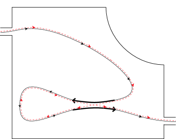
Abbildung 1: A Richter/Sieber pair of trajectories, contributing to conductance. The two trajectories connect leads attached to a chaotic cavity, and differ inside an antiparallel 2-encounter.

A lot of further interesting applications become accessible if the idea of encounter reconnections is applied to different types of trajectories. Doing so, it should be possible to go beyond the “threefold way” and extend the present results to the seven new symmetry classes [34], of experimental relevance for normal-metal/superconductor heterostructures and in quantum chromodynamics. First steps are taken in [64]. Here, the main quantity of interest is no longer the spectral form factor, but the level density proper. Classical orbits in a normal-conducting cavity attached to a superconductor have a peculiar form: Upon reflection from the surface of the superconductor, electrons are converted into holes, and vice versa. The analog of, say, a Sieber/Richter pair will be one single periodic orbit consisting of two subsequent parts. These parts differ (i) by reconnections inside a 2-encounter, and (ii) because one part describes the motion of an electron, whereas the other one describes the motion of a hole.

Transport properties such as conductance, shot noise, or delay times [65, 66, 67, 68, 69] provide another rich field of experimentally relevant applications. In the latter cases, the trajectories to be considered are no longer periodic, but connect two leads attached to a chaotic cavity. Conductance is determined by pairs of such trajectories [65]; in Fig. 1 we have depicted two trajectories differing in a 2-encounter. To study shot noise, one also has to take into account quadruples of trajectories [66].

While previous results were restricted to the lowest orders in series expansions of the quantities in question, our machinery of encounters and permutations, together with intuition drawn from field theory should allow to attack the full expansion. Moreover, the present formalism permits to elegantly treat general fully chaotic dynamics, and thus go beyond the model systems (like quantum graphs or the Hadamard-Gutzwiller model) employed in many of the above works.

Finally, our semiclassical treatment, applying to individual systems, should be capable of describing system-specific behavior and deviations from random-matrix theory, as long as these deviations are related to pairs of orbits differing in encounters. Deviations have been observed both for very small times (the corresponding range of $\tau$ shrinking to zero as $\hbar\to 0$), and around $\tau=1$ [70]. At least, we can explain the failure of random-matrix theory for $\tau<\frac{T_{E}}{T_{H}}$: In that regime, the present orbit pairs no longer exits, since the relevant encounter durations of order $T_{E}$ would exceed the orbit periods $\tau T_{H}$. Deviations from universality would also be of interest in the context of localization, and for dynamics with mixed phase space.

Chapter

Kapitel 8 Self-crossings in configuration space

Sieber’s and Richter’s seminal works [14, 15] on the $\tau^{2}$ contribution to spectral form factor were formulated in terms of self-crossings in configuration space, rather than close self-encounters in phase space. In [18], we extended this approach to general fully chaotic systems with two degrees of freedom and a Hamiltonian of the form $H({\bf q},{\bf p})=\frac{{\bf p}^{2}}{2m}+V({\bf q})$, by taking into account the geometry of the stable and unstable manifolds. In the following, we will first briefly review the analytical results of [18], stressing the connection to the treatment in Chapter 2. Thus prepared, we will then move on to numerical experiments and a more careful investigation of correction terms in the Hadamard-Gutzwiller model (the latter not included in [18]); for both extensions the language of self-crossings in configuration space seems to be better suited than the phase-space language employed in Chapter 2.

Anhang 8.A Overview

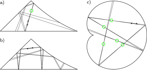
Abbildung 1: Configuration-space projections of phase-space encounters in the desymmetrized diamond and the cardioid billiard: a) containing one self-crossing (in a circle), b) narrowly avoiding a self-crossing, c) containing a “braid” of self-crossings (marked by circles) close to mutually conjugate points.

In (two-dimensional) configuration space, an antiparallel 2-encounter involves a self-crossing with a small angle $\epsilon$ as in Fig. 1a, or a narrowly avoided crossing as depicted in Fig. 1b. In systems with conjugate points, there can even be a “braid” of several small-angle crossings close to mutually conjugate points: Each crossing can be seen as the starting point of two close-by trajectories; these trajectories may meet again in points (almost) conjugate to the initial crossing and thereby form new crossings. An example for such a braid of self-crossings in the cardioid billiard is shown in Fig. 1c. These braids (as well as the almost self-retracing encounters discussed in Section 4) did not show up in the Hadamard-Gutzwiller model; they were first observed in [40] and treated analytically in [18].

Regardless of the system considered, in case of two dimensions at least one of the two partners in each Sieber/Richter pair involves a self-crossing. An investigation of self-crossings may therefore serve as a basis for determining the contribution of Sieber/Richter pairs to the spectral form factor.

To measure the separation between the two stretches of an encounter, we may use the small crossing angle $\epsilon$ rather than the stable and unstable coordinates $s$ and $u$. We can translate between both sets of coordinates by considering a Poincaré section ${\cal P}$ orthogonal to one of the encounter stretches at the location of a configuration-space crossing. This Poincaré section may be parametrized by configuration-space and momentum coordinates. The two stretches pierce through ${\cal P}$ in two almost mutually time-reversed phase-space points ${\bf x}_{1}$ and ${\bf x}_{2}$. Since ${\cal P}$ is placed at a crossing, the separation ${\cal T}{\bf x}_{2}-{\bf x}_{1}$ must have a vanishing configuration-space component. The momentum component may be written as $\pm|{\bf p}|\sin\epsilon$, or $\pm|{\bf p}|\epsilon$ in the limit of small crossing angles. Here $|{\bf p}|$ is the absolute value of the momentum part of either ${\bf x}_{1}$ or ${\bf x}_{2}$, and “$\pm$” has to be inserted because the angle $\epsilon$ will always be taken as positive. We thus obtain ${\cal T}{\bf x}_{2}-{\bf x}_{1}=\Big{(}{0\atop\pm|{\bf p}|\epsilon}\Big{)}$, the upper and lower lines respectively referring to configuration space and momentum space.

The separation $\Big{(}{0\atop\pm|{\bf p}|\epsilon}\Big{)}$ can be decomposed into one stable and one unstable part. Dropping the subscript of ${\bf x}\equiv{\bf x}_{1}$, we will characterize the stable and unstable directions ${\bf e}^{s}({\bf x})$, ${\bf e}^{u}({\bf x})$ at ${\bf x}$ by the ratios of their momentum and configuration-space components $B_{s}({\bf x})=\frac{e^{s}_{p}({\bf x})}{e^{s}_{q}({\bf x})}$ and $B_{u}({\bf x})=\frac{e^{u}_{p}({\bf x})}{e^{u}_{q}({\bf x})}$; these ratios are sometimes referred to as “curvatures” of the invariant manifolds [27]. The stable part of $\Big{(}{0\atop\pm|{\bf p}|\epsilon}\Big{)}$, denoted by $s{\bf e}^{s}({\bf x})$ in Chapter 2, is now given by

$$\mp\frac{|{\bf p}|\epsilon}{B_{u}({\bf x})-B_{s}({\bf x})}\Big{(}{1\atop B_{s}({\bf x})}\Big{)}\,,$$ (1)

whereas the unstable part reads

$$\pm\frac{|{\bf p}|\epsilon}{B_{u}({\bf x})-B_{s}({\bf x})}\Big{(}{1\atop B_{u}({\bf x})}\Big{)}\,;$$ (2)

as required, these parts are proportional to ${\bf e}^{s}({\bf x})\propto\Big{(}{1\atop B_{s}({\bf x})}\Big{)}$ and ${\bf e}^{u}({\bf x})\propto\Big{(}{1\atop B_{u}({\bf x})}\Big{)}$, respectively, and sum up to $\Big{(}{0\atop\pm|{\bf p}|\epsilon}\Big{)}$.

As in Chapter 2, the action difference $\Delta S=S_{\gamma}-S_{\gamma^{\prime}}$ between the partner orbits $\gamma$ and $\gamma^{\prime}$ ($\gamma$ now containing the crossing) is given by the symplectic product of the stable and unstable parts, i.e., by

$$\Delta S({\bf x},\epsilon)=\frac{|{\bf p}|^{2}\epsilon^{2}}{B_{u}({\bf x})-B_{s}({\bf x})}\,.$$ (3)

This result was originally derived in [18] using slightly different methods. In the special case of the Hadamard-Gutzwiller model, we have $B_{u}=-B_{s}=m\lambda$ and thus reproduce Sieber’s and Richter’s result $\Delta S=\frac{|{\bf p}|^{2}\epsilon^{2}}{2m\lambda}$ [14, 15].

Since crossing angles and stable and unstable coordinates are proportional, the encounter duration of Eq. (4) can be written as

$$t_{\rm enc}({\bf x},\epsilon)\sim\frac{2}{\lambda}\ln\frac{C({\bf x})}{\epsilon}\,.$$ (4)

The precise form of the proportionality factor $C({\bf x})$ is irrelevant for the following considerations. (Using that $t_{\rm enc}=\frac{1}{\lambda}\ln\frac{c^{2}}{|\Delta S|}$, see Eqs. (4) and (6), it is easy to show that $C({\bf x})$ depends on the bound $c$ and on the stable and unstable directions at ${\bf x}$ via $C({\bf x})=\frac{c}{|{\bf p}|}\sqrt{|B_{u}({\bf x})-B_{s}({\bf x})|}$). Note that we may not neglect the ${\bf x}$ dependence of $C({\bf x})$, since $t_{\rm enc}({\bf x},\epsilon)$ must be the same for all crossings inside a given encounter, even though these crossings involve different angles $\epsilon$. The durations $t_{s}$ and $t_{u}$ of the “tail” and “head” of the encounter can be expressed as similar logarithmic functions of $\epsilon$, albeit with different ${\bf x}$ dependent proportionality factors. For instance, $t_{u}$ may be written as

$$t_{u}({\bf x},\epsilon)\sim\frac{1}{\lambda}\ln\frac{C_{u}({\bf x})}{\epsilon}\,.$$ (5)

To count orbit pairs, we need to determine the density of self-crossings $P_{T}({\bf x},\epsilon)$, normalized such that integration over an interval of angles and a region inside the energy shell yields the corresponding number of self-crossings of one orbit of period close to $T$. Note that if we integrate over the whole energy shell, each crossing will be counted twice – once for each of the two almost time-reversed phase-space points. We include only crossings between encounter stretches separated by non-vanishing loops. Similarly as in Chapter 2, $P_{T}({\bf x},\epsilon)$ must be understood as averaged over all orbits with periods inside a small window around $T$.

To determine $P_{T}({\bf x},\epsilon)$, we start from a density of crossings with angles $\epsilon$, points ${\bf x}\equiv{\bf x}_{1}$ traversed at time $t_{1}$, and the point almost time-reversed with respect to ${\bf x}$ being traversed at time $t_{2}$. This density is defined such that integration over a region inside the energy shell and over intervals of $\epsilon$, $t_{1}$, and $t_{2}$ gives the pertaining number of crossings, averaged over the same ensemble of orbits as above. Using the ergodicity of the flow, one can show that this auxiliary density is given by

$$\frac{2|{\bf p}|^{2}\sin\epsilon}{m\Omega^{2}}\,.$$ (6)

Here, $\frac{1}{\Omega}$ represents the Liouville density on the energy shell (see Subsection 2), whereas the probability of finding a crossing in time intervals $(t_{1},t_{1}+dt_{1})$, $(t_{2},t_{2}+dt_{2})$ with angle inside an interval $(\epsilon,\epsilon+d\epsilon)$ is given by $\frac{2|{\bf p}|^{2}\sin\epsilon}{m\Omega}d\epsilon dt_{1}dt_{2}$. In particular, the factor $\sin\epsilon$ implies that orthogonal pieces of trajectory have a much higher probability to intersect than almost parallel ones. The derivation follows the lines of the Appendix of [14].

The desired density $P_{T}({\bf x},\epsilon)$ of phase-space points and crossing angles only is now obtained by integrating over $t_{1}$ and $t_{2}$. To include only encounters whose stretches are separated by intervening loops, we use the same restrictions on $t_{1}$, $t_{2}$ as in the phase-space calculation. We thus obtain

$$P_{T}({\bf x},\epsilon)=\frac{2|{\bf p}|^{2}\sin\epsilon}{m\Omega^{2}}T(T-2t_{\rm enc}({\bf x},\epsilon)),$$ (7)

with the correction term $\propto t_{\rm enc}$ due to the necessity of intervening loops.

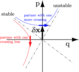
Abbildung 2: Poincaré section orthogonal to one of the encounter stretches of either $\gamma$ or $\gamma^{\prime}$, with lines indicating the stable and unstable directions and the vector $\delta{\bf x}$ pointing to the time-reversed of the other stretch. The picture shows the moment in which $\delta{\bf x}$ traverses the $p$-axis, i.e., the stretches cross in configuration space. The asymptotic motion of $\delta{\bf x}$ with respect to the invariant manifolds is indicated by arrows.

When evaluating the contribution to the spectral form factor, we have to make sure that each orbit pair is counted exactly once, even though the pertaining encounter may involve arbitrarily many self-crossings. To this end, we show that for general two-dimensional hyperbolic Hamiltonians of the form $H({\bf q},{\bf p})=\frac{{\bf p}^{2}}{2m}+V({\bf q})$ the numbers of crossings in the partner orbits $\gamma$ and $\gamma^{\prime}$ differ by one, the orbit with larger action containing one more crossing. This trivially applies to systems without conjugate points, where the partner with larger action contains one crossing and the other none. Our proof relies on an argument of winding numbers. We follow one of the two encounter stretches and study, in a Poincaré section orthogonal to the orbit, three quantities, the directions of the stable and unstable manifolds (which locally can be visualized as straight lines through the origin) and the small phase-space vector $\delta{\bf x}={\cal T}{\bf x}_{2}-{\bf x}_{1}$ pointing to the time reversed of the other encounter stretch; see Fig. 2. As we move along the orbit, these lines and vectors rotate around the origin, as in the treatment of the Maslov index in Sections 2 and 3. The encounter stretches cross in configuration space each time that $\delta{\bf x}$ rotates through the $p$-axis. Note that for Hamiltonians of the above form the $p$-axis may be traversed only in clockwise direction, given that $\dot{q}=\frac{p}{m}>0$ in the upper and $<0$ in the lower half plane.

For the orbit with larger action, our formula for the action difference demands that whenever a crossing occurs we have $B_{u}({\bf x})-B_{s}({\bf x})>0$, i.e., the unstable manifold has a higher slope in the Poincaré section than the stable one; $\delta{\bf x}$ is thus located between the stable manifold (on the counter-clockwise side) and the unstable manifold (on the clockwise side). The opposite applies to the partner with smaller action. For both orbits, the motion of $\delta{\bf x}$ is now given as a superposition of the rotation of the invariant manifolds and a motion from the stable towards the unstable manifold (since the stable components shrink and the unstable components grow). The motion towards the unstable manifold has clockwise sense for the partner with larger action, and counter-clockwise sense for the partner with smaller action. For the orbit with larger action, $\delta{\bf x}$ thus performs one more clockwise half-rotation around the orbit and therefore crosses the $p$-axis one more time. Consequently, the latter orbit indeed contains one more crossing.

To count each orbit pair exactly once, we have to weight crossings of the partners with larger and smaller action with respective positive and negative signs, by multiplying their contributions with $\mbox{sign}(B_{u}({\bf x})-B_{s}({\bf x}))$. As a result, only one contribution per orbit pair remains effective.

We can now evaluate the contribution of Sieber/Richter pairs $(\gamma,\gamma^{\prime})$ to the double sum for $K(\tau)$, see Eq. (25), replacing the sum over partners $\gamma^{\prime}$ by a sum over the self-crossings of $\gamma$. The latter sum may be written as an integral over $\epsilon$ and ${\bf x}$ with the density $P_{T}({\bf x},\epsilon)\mbox{sign}(B_{u}({\bf x})-B_{s}({\bf x}))$, as in

$$K_{\rm SR}(\tau) = \frac{2}{T_{H}}\left\langle\sum_{\gamma}|A_{\gamma}|^{2}\delta(\tau T_{H}-T_{\gamma})\right.\int d\mu({\bf x})\,\mbox{sign}(B_{u}({\bf x})-B_{s}({\bf x}))$$ (8)

$$\left.\ \ \ \ \times\int_{\epsilon>0}d\epsilon\,P_{\tau T_{H}}({\bf x},\epsilon)\cos\frac{\Delta S({\bf x},\epsilon)}{\hbar}\right\rangle,$$

As before, we have replaced $A_{\gamma^{\prime}}\to A_{\gamma}$, $T_{\gamma^{\prime}}\to T_{\gamma}$, and a factor 2 accounts for the time-reversed partner ${\cal T}\gamma^{\prime}$. (Two further factors mutually cancel: A factor 2 is needed because there is effectively one crossing per orbit pair – instead of one encounter in each $\gamma$ and $\gamma^{\prime}$. A factor $\frac{1}{2}$ compensates the inclusion of two almost time-reversed phase-space points ${\bf x}$ for each crossing.)

Similar the density $w_{\tau T_{H}}(s,u)$ of Chapter 2, $P_{\tau T_{H}}({\bf x},\epsilon)$ (compare Eq. (7)) falls into a leading term $\propto T_{H}^{2}$ and a subleading correction $\propto T_{H}t_{\rm enc}\sim T_{E}T_{H}$. When evaluating the $\epsilon$ integral in (8), the leading term yields a contribution scaling like $\hbar^{-1}$ in the semiclassical limit, and proportional to $\int d\epsilon\,\sin\epsilon\,\cos\frac{|{\bf p}|^{2}\epsilon^{2}}{(B_{u}({\bf x})-B_{s}({\bf x}))\hbar}$. If we approximate $\sin\epsilon\approx\epsilon$ for small angles, it is easy to show that the integral oscillates rapidly as $\hbar\to 0$ and thus vanishes after averaging.

The $\epsilon$ integral of the correction term gives $-\tau\frac{|B_{u}({\bf x})-B_{s}({\bf x})|}{2m\lambda\Omega}$. The absolute value is compensated by multiplication with $\mbox{sign}(B_{u}({\bf x})-B_{s}({\bf x}))$. Integrating over the energy shell, and applying the sum rule of Hannay and Ozorio de Almeida (12), we are led to

$$K_{\rm SR}(\tau)=-2\tau^{2}\frac{\,\overline{B_{u}-B_{s}}\,}{2m\lambda},$$ (9)

where $\overline{\rule{0.0pt}{5.8125pt}\ldots\rule{0.0pt}{5.8125pt}}$ denotes an average over the energy shell.

Now, ergodic theory needs to be invoked to relate the directions of the invariant manifolds to the Lyapunov exponent. The local stretching rate of a hyperbolic system depends on the normalization chosen for the stable and unstable direction ${\bf e}^{s}({\bf x})$ and ${\bf e}^{u}({\bf x})$. One of these choices [7] leads to $\chi({\bf x})=\frac{B_{u}({\bf x})}{m}$. Since the energy-shell average of $\chi({\bf x})$ coincides with the Lyapunov exponent of the system, we infer that $\overline{B_{u}}=m\lambda$. Moreover $B_{s}({\cal T}{\bf x})=-B_{u}({\bf x})$ implies that $\overline{B_{s}}=-\overline{B_{u}}=-m\lambda$. (Proofs for the special case of semi-dispersing billiards can also be found in [71]). From this, we immediately obtain the universal leading off-diagonal contribution to the spectral form factor

$$K_{\rm SR}(\tau)=-2\tau^{2}.$$ (10)

Anhang 8.B Numerical results

We have numerically investigated the statistics of self-crossings for two billiards, the desymmetrized diamond billiard and the cardioid billiard. For technical reasons, we considered non-periodic orbits, starting at time 0 and ending at time $T$. Each self-crossing is traversed at two times $t_{1}$, $t_{2}$ with $0<t_{1}<t_{2}<T$.

For both billiards, we want to concentrate on just one plot, displaying prominently a key idea of the present approach: The relevant encounters must have their stretches separated by intervening loops. The time interval between $t_{1}$ and $t_{2}$ is large enough to contain a non-vanishing loop only if time difference $\delta t=t_{2}-t_{1}$ exceeds the logarithmic threshold $2t_{u}({\bf x},\epsilon)\sim\frac{2}{\lambda}\ln\frac{C_{u}({\bf x})}{\epsilon}$; see Eqs. (12) and (5). Since in case of non-periodic trajectories there can be no second loop, the traversal times do not have to obey any further restrictions (like Eq. (13) for periodic orbits). To illustrate the threshold for $\delta t$, we consider a combined density $P_{T}({\bf x},\epsilon,\delta t)$ of crossing points, angles, and time differences in non-periodic orbits of duration $T$. Similarly to the preceding Subsection, an analytical prediction can be made if we integrate over the auxiliary density in Eq. (6). We then obtain

$$P_{T}({\bf x},\epsilon,\delta t) = \int_{0}^{T}dt_{2}\int_{0}^{t_{2}}dt_{1}\,\delta(\delta t-(t_{2}-t_{1}))\Theta(\delta t-2t_{u}({\bf x},\epsilon))\frac{2|{\bf p}|^{2}\sin\epsilon}{m\Omega^{2}}$$ (11)

$$= \frac{2|{\bf p}|^{2}\sin\epsilon}{m\Omega^{2}}(T-\delta t)\Theta(\delta t-2t_{u}({\bf x},\epsilon))\,,$$

where the $\Theta$ function originates from the minimal time difference $2t_{u}({\bf x},\epsilon)$.

Similarly as in Section 5 we expect slight deviations from the ergodic crossing probability (6) and thus from (11) for encounter stretches separated by loops shorter than the classical relaxation time $t_{\rm cl}$, since in this case both stretches are statistically correlated; such deviations will concern time differences $\delta t$ just slightly exceeding the minimum $2t_{u}({\bf x},\epsilon)$.

Densities of other sets of parameters were investigated in [40] in a preliminary version and in [18] in final form.

Desymmetrized diamond billiard

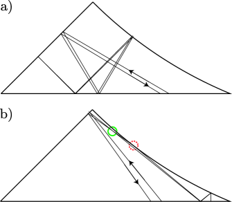
Abbildung 3: Exceptional encounters in the desymmetrized diamond billiard: a) an almost self-retracing encounter without small-angle crossings, b) an example for a crossing (in the full circle) related to the tangential singularity; in the dotted circle, one stretch narrowly misses the boundary whereas the other one undergoes a glancing reflection.

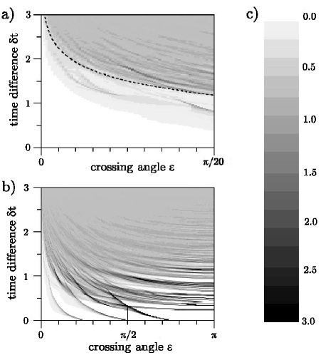
Abbildung 4: Plot of the combined density of time differences $\delta t$ and crossing angles $\epsilon$ in the desymmetrized diamond billiard: a) for $\epsilon<\frac{\pi}{20}$, b) for all angles, for non-periodic orbits of duration $T=10$. Normalization as defined in the text; the resulting scale is shown in c). For small angles, we observe a threshold logarithmic in $\epsilon$, as indicated by a dashed line.

We have first checked Eq. (11) for the desymmetrized diamond billiard. Here all self-crossings belong to encounters separated by loops. Almost self-retracing encounters as in Fig. 3a may not involve self-crossings, since these would have to be conjugate to the reflection point. Hence, encounters without a partner are automatically excluded from our statistics. The same applies to all systems without conjugate points.

Consider Fig. 4 for a density plot of crossing angles and time differences, for crossing points ${\bf x}$ anywhere on the energy shell. The plot depicts the density $P_{T}({\bf x},\epsilon,\delta t)$, after dividing out $\sin\epsilon$ and integrating over the energy shell. The results were obtained by averaging over $2\times 10^{7}$ non-periodic trajectories with random initial conditions and duration $T=10$, measured in dimensionless coordinates with mass and velocity equal to one.

For small angles, the existence of a minimal time difference depending logarithmitically on the crossing angle can be verified by a glance at Fig. 4a. Here, the dashed line represents the minimal time difference $2t_{u}({\bf x},\epsilon)\sim\frac{2}{\lambda}\ln\frac{C_{u}({\bf x})}{\epsilon}$, with $C_{u}({\bf x})$ replaced by a constant obtained through numerical fitting. Sufficiently far above the logarithmic curve, the density is almost uniform. In agreement with Eq. (11), it decays linearly towards larger $\delta t$. Below the dashed line, the density of crossings diminishes fast before vanishing completely inside the white region.

In the vicinity of the logarithmic curve, i.e., for short loops, deviations from the ergodic crossing probability of Eq. (6) make for system-specific inhomogeneities. Furthermore, the threshold is smeared out since, rather than exactly following the dashed line, the minimal time difference weakly depends on the location on the energy shell through the factor $C_{u}({\bf x})$ in Eq. (5).

Most of the crossings significantly below the latter line are due to a system-specific effect, related to the tangential singularity of the billiard flow: The linear approximation for the separation between the two encounter stretches is already violated if one stretch is reflected at the circular part of the boundary, and the other stretch narrowly avoids the circle; see Fig. 3b for an example. The encounter should be considered to end at this reflection point, even if the phase-space separation between the two stretches is still very small. Hence the duration of the “head” of the encounter $t_{u}$ is much shorter than $\frac{1}{\lambda}\ln\frac{C_{u}({\bf x})}{\epsilon}$. The time difference $\delta t$ between two traversals of the crossing may thus remain far below the logarithmic threshold, like in the example of Fig. 3b. However, our numerical results indicate that the resulting effect on the crossing distribution is minute, since these exceptional crossings are much less numerous than generic ones.

At larger angles, which in the semiclassical limit have no impact on the form factor, Fig. 4b shows further system-specific structures. Discrete lines at $\epsilon=\pi$ correspond to periodic orbits, since by “crossing” itself at an angle $\pi$, an orbit simply closes in phase space. These lines are deformed and broadened when going to smaller angles. Thus, most “orbit parts” (i.e., pieces of trajectory between two traversals of a crossing) close to $\delta t\approx 2t_{u}$ are obtained by deformation of the shortest periodic orbits. In contrast, the families of “orbit parts” starting at $\delta t=0$ are related to the corners of the billiard [40, 18].

Cardioid billiard

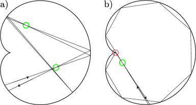
Abbildung 5: Encounters in the cardioid billiard: a) an almost self-retracing encounter containing crossings (marked by circles) almost conjugate to the reflection point, b) example for a cusp-related crossing; in the dotted circle, only one of the two stretches is reflected.

As a second example, we consider the cardioid billiard. In the cardioid, almost self-retracing encounters may involve crossings, as seen in Fig. 5a. The locations of these crossings are conjugate to each other, and to the point where the orbit is reflected from the wall with an almost right angle: The two traversals of each crossing limit a fan of trajectories with a small opening angle which gathers again in the remaining crossings and in the reflection point. Since there is no associated partner orbit, these crossings have to be excluded from our statistics, using a criterion based on symbolic dynamics. We determine the symbol sequence of the orbit and look for the pair of mutually time-reversed subsequences $\ldots{\cal E}\ldots\bar{{\cal E}}\ldots$, representing the encounter in question. We consider only crossings for which ${\cal E}$ and $\overline{{\cal E}}$ are separated by a subsequence ${\cal R}$ representing an intervening loop; the sequence ${\cal R}$ may not be time-reversal invariant, since otherwise it could be included in ${\cal E}$.

An example for a further class of system-specific crossings is given in Fig. 5b. The depicted encounter ends abruptly when one of the two stretches is reflected close to the cusp of the billiard, while the second stretch narrowly avoids the cusp. The following loop remains close to the boundary of the billiard and undergoes several almost glancing reflections. Since the orbit in question comes extremely close to the classically forbidden region, the applicability of the Gutzwiller trace formula is highly questionable. We thus eliminate such crossings from our statistics as well [18].

The statistics of the remaining crossings confirms our predictions. Again, the density of crossing angles and time differences, Fig. 6, reveals a threshold for $\delta t$ depending logarithmitically on the angle, and some system-specific inhomogeneities close to that threshold.

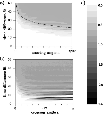
Abbildung 6: Plot of the combined density of time differences $\delta t$ and crossing angles $\epsilon$ in the cardioid billiard: a) for $\epsilon<\frac{\pi}{20}$, b) for all angles. Normalization as explained in the text and used in Fig. 4; the resulting scale is shown in c). For small angles, we observe a threshold logarithmic in $\epsilon$, as indicated by a dashed line.

Like in case of the desymmetrized diamond, these system-specific features do not prevent universal behavior in the semiclassical limit, since they are associated to classical time scales negligible compared to $T_{E}$ and $T_{H}$. A better understanding of these features could, nevertheless, be helpful for mathematically rigorous work or for studying deviations from universality outside the semiclassical limit. Note that the Hadamard-Gutzwiller model also displays system-specific structures, but of a different kind: In that model, the analog of Figs. 4 and 6 just consists of dispersionless logarithmic curves corresponding each to the family of orbit parts obtained by deformation of one periodic orbit [15].

Anhang 8.C Sieber/Richter pairs give no additional contributions

We have seen that Sieber/Richter pairs contribute to the spectral form factor only through a correction term inside $P_{T}({\bf x},\epsilon)$, of subleading order in the orbit period. Could a more careful analysis of these orbit pairs reveal further corrections, also affecting the form factor?

In the following, we shall identify several such corrections, but show that their contributions to the form factor mutually cancel. We will restrict ourselves to the Hadamard-Gutzwiller model, i.e., a surface of constant negative curvature, tesselated into octagonic pieces [72, 16, 17, 54]. This model is homogeneously hyperbolic, i.e., the local stretching rates $\chi({\bf x})$ of all phase-space points ${\bf x}$ and the Lyapunov exponents $\lambda_{\gamma}$ of all periodic orbits coincide with the Lyapunov exponent of the system $\lambda$. As a consequence, we have $B_{u}({\bf x})=-B_{s}({\bf x})=m\lambda$, and may neglect the ${\bf x}$ dependence of $C({\bf x})$. Thus, when investigating the statistics of encounters, we need not discriminate between different points on the energy shell. To formulate that statistics, we work in dimensionless units with $m=|{\bf p}|=\lambda=1$; in these units length, period, and action of each orbit coincide, and will collectively be denoted by $L$; likewise we will replace $t_{\rm enc}\to l_{\rm enc}$, $T_{H}\to L_{H}$, and $\Delta S\to\Delta L$. We then obtain a density of crossing angles only,

$$P_{L}(\epsilon)=\frac{\sin\epsilon}{\Omega}L(L-2l_{\rm enc}(\epsilon))\,,$$ (12)

and Eq. (8) turns into

$$K_{\rm SR}(\tau)=\frac{4}{L_{H}}\left\langle\sum_{\gamma}\int_{\epsilon>0}d\epsilon\,A_{\gamma}A_{\gamma^{\prime}}\delta\left(\tau L_{H}-\frac{L_{\gamma}+L_{\gamma^{\prime}}}{2}\right)P_{L_{\gamma}}(\epsilon)\cos\frac{\Delta L}{\hbar}\right\rangle\,.$$ (13)

Here, we deliberately avoided to replace $A_{\gamma^{\prime}}\to A_{\gamma}$, or $L_{\gamma^{\prime}}\to L_{\gamma}$, and dropped the phases of $A_{\gamma}$ and $A_{\gamma^{\prime}}$ since the corresponding Maslov indices coincide. (The Maslov indices even vanish, unless we divide the Hadamard-Gutzwiller model into pieces in order to remove its symmetry.) Compared to Eqs. (7) and (8), a factor 2 was shifted from the density (12) to the prefactor in Eq. (13), since $P_{L}(\epsilon)$ does not discriminate between the two points of traversal and thus accounts for each crossing only once.

When evaluating (13), we want to avoid the potentially dangerous approximations made in Chapter 2 and in Appendix 8.A. Three points require special care:

• We need to take into account the difference between the stability amplitudes $A_{\gamma}$ and $A_{\gamma^{\prime}}$. To do so, we write

  $$A_{\gamma}=\frac{T_{\gamma}}{\sqrt{|\det(M_{\gamma}-1)|}}=\frac{T_{\gamma}}{2\sinh\frac{\lambda_{\gamma}T_{\gamma}}{2}}=\frac{L_{\gamma}}{2\sinh\frac{L_{\gamma}}{2}}\stackrel{{\scriptstyle L_{\gamma}\gg 1}}{{\approx}}L_{\gamma}{\rm e}^{-L_{\gamma}/2}\,,$$ (14)

  see Eq. (11), and express $A_{\gamma^{\prime}}$ as

  $$A_{\gamma^{\prime}}\approx\frac{L_{\gamma^{\prime}}}{L_{\gamma}}{\rm e}^{\Delta L/2}A_{\gamma}=\left(1-\frac{\Delta L}{L_{\gamma}}\right){\rm e}^{\Delta L/2}A_{\gamma}\,,$$ (15)

  depending on the length difference between $\gamma$ and $\gamma^{\prime}$, $\Delta L=L_{\gamma}-L_{\gamma^{\prime}}$.

• When treating the length (or action) difference, hyperbolic geometry allows to go beyond Sieber’s and Richter’s approximation $\Delta L\approx\frac{\epsilon^{2}}{2}$. As shown in [17], we have $\Delta L=-4\ln\cos\frac{\epsilon}{2}=\frac{\epsilon^{2}}{2}+\frac{\epsilon^{4}}{48}+\ldots$.

• Finally, we work with the exact crossing density $P_{L}(\epsilon)$, without replacing $\sin\epsilon=\epsilon-\frac{\epsilon^{3}}{3}+\ldots$ by $\epsilon$.

The three corrections mentioned involve only higher orders in $\epsilon$. Upon applying $\int d\epsilon\,{\rm e}^{{\rm i}\epsilon^{2}/(2\hbar)}\ldots$ the resulting contributions to the form factor will be of higher order in $\hbar$, each factor $\epsilon^{2}$ being turned into a factor proportional to $\hbar$. Therefore, the changes arising will not affect the contribution of the correction term inside $P_{L}(\epsilon)$, originating form the necessity of intervening loops. The latter correction term still yields $K_{\rm SR,corr}(\tau)=-2\tau^{2}$. We must, however, reexamine the contribution of the leading term $\propto L^{2}$. In Appendix 8.A, that term gave a contribution scaling like $\hbar^{-1}$, but vanishing after averaging. Additional corrections of relative order $\hbar$ therefore have a chance to survive in the semiclassical limit. In contrast, the length difference $\Delta L\propto\epsilon^{2}$, effectively of order $\hbar$, can be safely neglected when directly compared to the orbit period $L_{\gamma^{\prime}}\propto\hbar^{-1}$. We hence drop the summand $\frac{\Delta L}{L_{\gamma}}$ in (15) and replace $\frac{L_{\gamma}+L_{\gamma^{\prime}}}{2}\to L_{\gamma}$ in the $\delta$-function of Eq. (13). Altogether, we thus obtain

$$K_{{\rm SR,lead}}(\tau) = \frac{4}{L_{H}}\left\langle\sum_{\gamma}A_{\gamma}^{2}\,\delta(\tau L_{H}-L_{\gamma})\int_{\epsilon>0}d\epsilon\,{\rm e}^{\Delta L/2}\left(\frac{\sin\epsilon}{\Omega}L_{\gamma}^{2}\right)\cos\frac{\Delta L}{\hbar}\right\rangle$$ (16)

$$= 4\tau^{3}\frac{L_{H}^{2}}{\Omega}\left\langle\int_{\epsilon>0}d\epsilon\,{\rm e}^{\Delta L/2}\sin\epsilon\,\cos\frac{\Delta L}{\hbar}\right\rangle,$$

where in the final step we have used the sum rule of Hannay and Ozorio de Almeida.

The remaining integral can be evaluated by transforming to $\Delta L=-4\ln\cos\frac{\epsilon}{2}$ as a new integration variable. After simplifying the integrand of Eq. (16),

$$d\epsilon\,{\rm e}^{\Delta L/2}\sin\epsilon = d\Delta L\left(\frac{d\Delta L}{d\epsilon}\right)^{-1}{\rm e}^{\Delta L/2}\sin\epsilon$$ (17)

$$= d\Delta L\left(2\tan\frac{\epsilon}{2}\right)^{-1}\left(\cos\frac{\epsilon}{2}\right)^{-2}\left(2\sin\frac{\epsilon}{2}\cos\frac{\epsilon}{2}\right)$$

$$= d\Delta L\,,$$

we find

$$K_{{\rm SR,lead}}(\tau)=4\tau^{3}\frac{L_{H}^{2}}{\Omega}\left\langle\int_{0}^{\Delta L_{\rm max}}d\Delta L\cos\frac{\Delta L}{\hbar}\right\rangle=4\tau^{3}\frac{L_{H}^{2}\hbar}{\Omega}\left\langle\sin\frac{\Delta L_{\rm max}}{\hbar}\right\rangle\,.$$ (18)

Here $\Delta L_{\rm max}$ is the maximal length difference considered, analogous to the maximal action difference $c^{2}$ following from $|s|,|u|<c$ in Chapter 2. The resulting sine oscillates rapidly in the semiclassical limit, and is annihilated by averaging. We thus see that the additional corrections do not affect the spectral form factor.

To achieve this result, it was of crucial importance to include all three corrections listed, of order $O(\epsilon^{2})$ compared to the terms considered in [14, 15]. Each single correction would yield a non-vanishing contribution of order $\tau^{3}$. However, Eq. (18) implies that all three corrections taken together mutually cancel.

Anhang 8.D Summary

We reviewed an alternative treatment of Sieber/Richter pairs, determining the $\tau^{2}$ contribution to the form factor. This alternative approach was based on self-crossings in two-dimensional configuration space and the geometry of the stable and unstable manifolds in phase space. Each encounter contains one or more self-crossings, or a narrowly avoided crossing. The action difference can be expressed as a function of the crossing angle and the stable and unstable directions at the location of the crossing. Numerical investigations clearly demonstrate that the stretches of the relevant encounters are separated by loops, and therefore the traversals of the relevant crossings have minimal time differences logarithmic in the crossing angle. Moreover, our plots show some system-specific structures related to very short loops. We finally presented a more careful analysis of Sieber/Richter pairs in the Hadamard-Gutzwiller model, showing that three additional correction terms give mutually canceling contributions to the form factor.

Kapitel 9 Integrals involving $1/t_{\rm enc}$

We want to evaluate the integral

$$\int_{-c}^{c}d^{l-1}sd^{l-1}u\frac{1}{t_{\rm enc}(s,u)}{\rm e}^{{{\rm i}}\Delta S/\hbar}$$ (1)

over the $2(l-1)$ stable and unstable separations $s_{j}$, $u_{j}$ inside an $l$-encounter. These variables determine both the duration $t_{\rm enc}(s,u)$ of the encounter in question and its contribution to the action difference $\Delta S=\sum_{j}s_{j}u_{j}$. We shall show that the integral oscillates rapidly as $\hbar\to 0$ and thus may be neglected in the semiclassical limit. This was required in Section 5 to show that certain terms in the multinomial expansion of $w_{T}(s,u)$ do not contribute to the form factor; the special case $l=2$ was treated in Section 6.

The key is the following change of picture: So far, all Poincaré sections ${\cal P}$ inside a given encounter were integrated over; we thus had to divide out the duration $t_{\rm enc}$. Instead, we may single out a section ${\cal P}^{{\rm e}}$, fixed at the end of the encounter, and only consider the stable and unstable separations $s_{j}^{{\rm e}}$, $u_{j}^{{\rm e}}$ therein. For homogeneously hyperbolic dynamics, i.e., $\Lambda({\bf x},t)={\rm e}^{\lambda t}$ for all ${\bf x}$ and $t$, the separations inside ${\cal P}^{{\rm e}}$ are given by $s_{j}^{{\rm e}}=s_{j}{\rm e}^{-\lambda t_{u}}$, $u_{j}^{{\rm e}}=u_{j}{\rm e}^{\lambda t_{u}}$ with $t_{u}$ denoting the time difference between ${\cal P}$ and ${\cal P}^{{\rm e}}$.

We recall that the encounter ends when the largest of the unstable components, say the $J$th one, reaches $\pm c$ such that $u_{J}^{{\rm e}}=u_{J}{\rm e}^{\lambda t_{u}}=\pm c$. All $l-1$ possibilities $J=1,2,\ldots,l-1$ and the two possibilities for the sign $u_{J}^{{\rm e}}/c=\pm 1$ give additive contributions $I_{J}^{\pm}$ to the integral (1). Each of these contributions is easily evaluated after transforming the integration variables from $s_{j}$, $u_{j}$ to $s_{j}^{{\rm e}}$, $u_{j}^{{\rm e}}$ (with $j\neq J$), $s_{J}^{{\rm e}}$, and $t_{u}=\frac{1}{\lambda}\ln\frac{c}{|u_{J}|}$. The Jacobian of that transformation equals $\lambda c$. The new coordinates determine the action difference as $\Delta S=\sum_{j}s_{j}^{{\rm e}}u_{j}^{{\rm e}}=\sum_{j\neq J}s_{j}^{{\rm e}}u_{j}^{{\rm e}}\pm s_{J}^{{\rm e}}c$. The encounter duration is given by $t_{\rm enc}(s,u)=t_{\rm enc}(s^{\rm e},u^{\rm e})=\min_{j}\Big{\{}\frac{1}{\lambda}\ln\frac{c}{|s^{\rm e}_{j}|}\Big{\}}$, see Eq. (4). Note that $t_{\rm enc}$ does not depend on the unstable coordinates $u^{\rm e}$; the latter determine only the duration of the encounter head, which is missing because the Poincaré section ${\cal P}^{\rm e}$ is placed in the end of the encounter. Since our new coordinates are restricted to the ranges $-c<s_{j}^{{\rm e}}<c$, $-c<u_{j}^{{\rm e}}<c$, for $j\neq J$, $-c<s_{J}^{{\rm e}}<c$, and $0<t_{u}<t_{\rm enc}$, we obtain

$$I_{J}^{\pm} = \lambda c\int_{-c}^{c}ds_{J}^{{\rm e}}{\rm e}^{\pm{\rm i}s_{J}^{{\rm e}}c/\hbar}\left(\prod_{j\neq J}\int_{-c}^{c}ds_{j}^{{\rm e}}du_{j}^{{\rm e}}{\rm e}^{{\rm i}s_{j}^{{\rm e}}u_{j}^{{\rm e}}/\hbar}\right)$$ (2)

$$\times\underbrace{\frac{1}{t_{\rm enc}(s^{{\rm e}},u^{{\rm e}})}\int_{0}^{t_{\rm enc}(s^{{\rm e}},u^{{\rm e}})}dt_{u}}_{=1}$$

$$\sim \lambda(2\pi\hbar)^{l-2}2\hbar\sin\frac{c^{2}}{\hbar}\,.$$

Note that the divisor $t_{\rm enc}$ was canceled by the $t_{u}$ integral; moreover, the $2(l-2)$ integrals over $s_{j}^{{\rm e}},u_{j}^{{\rm e}}$, of the form already encountered in Eq. (24), gave the factor $(2\pi\hbar)^{l-2}$. Most importantly, the factor $\sin\frac{c^{2}}{\hbar}$, provided by the integral over $s_{J}^{{\rm e}}$, is a rapidly oscillating function of $c$ and $\hbar$, annulled by averaging over these quantities; as shown in Section 6 averaging over $c$ is equivalent to averaging over the energy $E$. Thus, the integral (1), just the $2(l-1)$-fold of Eq. (2), effectively vanishes as $\hbar\to 0$. Note that rapidly oscillating terms as in Eq. (2) are essentially spurious and would not appear if smooth encounter cut-offs were used (instead of our $|s|<c,|u|<c$).

Kapitel 10 Extension to general hyperbolicity and $f>2$

So far, some of our reasoning was restricted to two-dimensional homogeneously hyperbolic systems. Here, we extend our approach to general fully chaotic dynamics with arbitrary numbers $f$ of degrees of freedom. The present results were published in [21] for the case of Sieber/Richter pairs, and in an Appendix of [22] for arbitrary orders in $\tau$.

Anhang 10.A General hyperbolicity

First, we drop the restriction to “homogeneously hyperbolic” dynamics, for which all phase space points ${\bf x}$ have the same Lyapunov exponent $\lambda$ and the same stretching factor $\Lambda(t)={\rm e}^{\lambda t}$. We extend our reasoning to general hyperbolic systems, where the stretching factors $\Lambda({\bf x},t)$ may depend on ${\bf x}$. In such systems the Lyapunov exponents of almost all points still coincide with the ${\bf x}$ independent “Lyapunov exponent of the system”, whereas each periodic orbit may come with its own Lyapunov exponent (see Section 1).

Most importantly, the divergence of the stretches involved in an encounter depends on the local stretching factor of that encounter, rather than the Lyapunov exponent of the system. Consequently, our formula (4) for the encounter duration can only be read as an approximation, and that approximation is now to be avoided. We will thus allow the duration $t_{\rm enc}^{\alpha}$ of the $\alpha$-th encounter to depend not only on the stable and unstable separations $s_{\alpha j}$, $u_{\alpha j}$, but also on the phase-space location of the piercing ${\bf x}_{\alpha 1}$ chosen as the origin of the corresponding Poincaré section. Together, the reference piercing ${\bf x}_{\alpha 1}$ and the separations $s_{\alpha j}$, $u_{\alpha j}$ determine the positions of all piercing points of the $\alpha$-th encounter and therefore clearly suffice to determine its duration. The changes arising will be important only for showing that the contribution originating from the $\frac{1}{t_{\rm enc}}$-integrals of Appendix 9 vanishes; recall that the reasoning in Appendix 9 explicitly required homogeneous hyperbolicity. In contrast, the terms contributing to $K(\tau)$ remain unaffected, since for these terms all occurrences of $t_{\rm enc}$ mutually cancel.

When generalizing the statistics of encounters of Section 4, we must extend $w_{T}(s,u)$ to a density $w_{T}({\bf x},s,u)$ also depending on the points of the reference piercings ${\bf x}=\{{\bf x}_{11},{\bf x}_{21},\ldots,{\bf x}_{V1}\}$. We assume that all piercing points are statistically uncorrelated; as we have seen, the only existing correlations are related to loops shorter than the classical relaxation time $t_{\rm cl}\ll T_{E}$ and thus cannot affect the spectral form factor. We therefore expect a density of reference piercings and stable and unstable coordinates

$$w_{T}({\bf x},s,u)=\frac{T(T-\sum_{\alpha}l_{\alpha}t_{\rm enc}^{\alpha})^{L-1}}{(L-1)!\Omega^{L}\prod_{\alpha}t_{\rm enc}^{\alpha}}\,,$$ (1)

differing from the $w_{T}(s,u)$ of Eq. (10) only by $t_{\rm enc}^{\alpha}=t_{\rm enc}^{\alpha}({\bf x}_{\alpha 1},s_{\alpha},u_{\alpha})$ being a function of ${\bf x}_{\alpha 1}$, and by a factor $\frac{1}{\Omega^{V}}$ arising from the Liouville density for each of the $V$ reference piercings. Our expression for the form factor, Eq. (14), now turns into

$$K(\tau)=\kappa\tau+\kappa\tau\left\langle\sum_{\vec{v}}\frac{N(\vec{v})}{L}\int d^{V}\mu({\bf x})\int d^{L-V}s\;d^{L-V}u\;w_{T}({\bf x},s,u)\;{\rm e}^{\rm i\Delta S/\hbar}\right\rangle,$$ (2)

where the ${\bf x}$ integral refers to $V$ points ${\bf x}_{\alpha 1}$ in the energy shell, i.e., $d^{V}\mu({\bf x})=\prod_{\alpha=1}^{V}d^{4}x_{\alpha 1}\,\delta(H({\bf x}_{\alpha 1})-E)$. Eqs. (1) and (2) can easily be justified along the lines of Chapter 4. In the following we want, however, to give a mathematically more careful derivation, showing explicitly how the equidistribution theorem of [26] and the condition of mixing come into play.

Derivation of Eqs. (1) and (2)

We first want to consider encounters of one single periodic orbit $\gamma$. To do so, we choose an arbitrary “starting point” ${\bf z}_{0}$ on $\gamma$, and let $\Phi_{t}({\bf z}_{0})$ denote the image of ${\bf z}_{0}$ under evolution over the time $t$. For the moment, we want to restrict ourselves to systems without time-reversal invariance.

We now generalize the density $\rho(s,u,t)$ of Eq. (8) to a density $\rho^{\gamma}({\bf x},s,u,t)$ of piercing times $t_{\alpha j}$, reference piercings ${\bf x}_{\alpha 1}=\Phi_{t_{\alpha 1}}({\bf z}_{0})$, and stable and unstable coordinates $s$, $u$ associated to $\hat{s}$, $\hat{u}$ with $\Phi_{t_{\alpha j}}({\bf z}_{0})-{\bf x}_{\alpha 1}=\hat{s}_{\alpha j}{\bf e}^{s}({\bf x}_{\alpha 1})+\hat{u}_{\alpha j}{\bf e}^{u}({\bf x}_{\alpha 1})$. The density $\rho^{\gamma}({\bf x},s,u,t)$ shall refer to a fixed orbit $\gamma$, a fixed structure of the orbit pair $(\gamma,\gamma^{\prime})$ and fixed times $t_{\alpha 1}$ of the reference piercings; it will be normalized such that integration over energy-shell regions for the reference piercings ${\bf x}_{\alpha 1}$, and over intervals for the stable and unstable coordinates $s_{\alpha j}$, $u_{\alpha j}$ ($j=1,\ldots,l_{\alpha}-1$) and the remaining piercing times $t_{\alpha j}$ (now with $j$ running $j=2,\ldots,l_{\alpha}$) yields the corresponding number of sets of piercings inside $\gamma$. For each orbit $\gamma$, the $\rho^{\gamma}({\bf x},s,u)$ thus defined can be written as a product of $\delta$ functions,

$$\rho^{\gamma}({\bf x},s,u,t)=\Theta_{T}({\bf x},s,u,t)\prod_{\alpha=1}^{V}\delta(\Phi_{t_{\alpha 1}}({\bf z}_{0})-{\bf x}_{\alpha 1})$$

$$\ \ \ \ \ \ \times\prod_{j=2}^{l_{\alpha}}\delta\left(\Phi_{t_{\alpha j}}({\bf z}_{0})-{\bf x}_{\alpha 1}-\hat{s}_{\alpha j}{\bf e}^{s}({\bf x}_{\alpha 1})-\hat{u}_{\alpha j}{\bf e}^{u}({\bf x}_{\alpha 1})\right).$$ (3)

This product also involves a characteristic function $\Theta_{T}({\bf x},s,u,t)$ which returns 1 if the ordering of times corresponds to the structure considered and the time differences suffice to have all encounter stretches separated by loops; otherwise $\Theta_{T}({\bf x},s,u,t)$ is equal to zero. Eq. (10.A) can easily be generalized to time-reversal invariant systems: If the $j$-th stretch of the $\alpha$-th encounter is almost time-reversed with respect to the first one, we simply have to replace $\Phi_{t_{\alpha j}}({\bf z}_{0})\to{\cal T}\Phi_{t_{\alpha j}}({\bf z}_{0})$.

In analogy to Section 4, we integrate over the piercing times and divide out the encounter durations, obtaining a density of reference piercings and stable and unstable separations only,

$$w^{\gamma}({\bf x},s,u)=\frac{\int d^{L}t\ \rho^{\gamma}({\bf x},s,u,t)}{\prod_{\alpha}t_{\rm enc}^{\alpha}({\bf x}_{\alpha 1},s_{\alpha},u_{\alpha})}.$$ (4)

The periodic-orbit sum for the spectral form factor (14) now takes the form

$$K(\tau)=\kappa\tau+\frac{\kappa}{T_{H}}\left\langle\sum_{\vec{v}}\frac{N(\vec{v})}{L}\int d^{V}\mu({\bf x})\int d^{L-V}s\;d^{L-V}u\;{\rm e}^{{\rm i}\Delta S/\hbar}\right.$$

$$\ \ \ \ \ \ \ \ \ \ \ \ \ \ \ \ \ \ \ \ \ \ \ \ \ \ \times\left.\left\{\sum_{\gamma}|A_{\gamma}|^{2}\delta(T-T_{\gamma})w^{\gamma}({\bf x},s,u)\;\right\}\right\rangle.$$ (5)

The form factor thus depends on the average

$$\frac{1}{T}\left\langle\sum_{\gamma}|A_{\gamma}|^{2}\delta(T-T_{\gamma})w^{\gamma}({\bf x},s,u)\;\right\rangle_{\!\!\!\Delta T}$$ (6)

of $w^{\gamma}({\bf x},s,u)$ over the ensemble of all periodic orbits with periods inside a small window around $T$, weighted with the square of their stability amplitudes. We have to show that this average coincides with the $w_{T}({\bf x},s,u)$ of Eq. (1).

To proceed, we split the time integral of Eq. (4) into an integral over $0<t_{11}<T$, and further integrals over the differences $t_{\alpha j}^{\prime}=t_{\alpha j}-t_{11}$ of all other piercing times from the first one. Using that $\Phi_{t_{\alpha j}}({\bf z}_{0})=\Phi_{t_{11}+t_{\alpha j}^{\prime}}({\bf z}_{0})=\Phi_{t_{11}}(\Phi_{t_{\alpha j}^{\prime}}({\bf z}_{0}))$, we may thus represent $w^{\gamma}$ as the average of an observable $f({\bf z})$ along $\gamma$,

$$w^{\gamma}({\bf x},s,u)=\frac{1}{T}\int_{0}^{T}dt_{11}\,f(\Phi_{t_{11}}({\bf z}_{0}))\equiv\big{[}f\big{]}_{\gamma}$$ (7)

with

$$f({\bf z}) = \frac{T}{\prod_{\alpha}t_{\rm enc}^{\alpha}({\bf x}_{\alpha 1},s_{\alpha},u_{\alpha})}\int d^{L-1}t^{\prime}\,\Theta_{T}({\bf x},s,u,t^{\prime})\prod_{\alpha=1}^{V}\delta(\Phi_{t_{\alpha 1}^{\prime}}({\bf z})-{\bf x}_{\alpha 1})$$ (8)

$$\times\prod_{j=2}^{l_{\alpha}}\delta\left(\Phi_{t_{\alpha j}^{\prime}}({\bf z})-{\bf x}_{\alpha 1}-\hat{s}_{\alpha j}{\bf e}^{s}({\bf x}_{\alpha 1})-\hat{u}_{\alpha j}{\bf e}^{u}({\bf x}_{\alpha 1})\right)\,.$$

Here were replaced $\Theta_{T}({\bf x},s,u,t)\to\Theta_{T}({\bf x},s,u,t^{\prime})$, since the times $t_{\alpha j}^{\prime}=t_{\alpha j}-t_{11}$ have to obey the same ordering and the same minimal distances as the times $t_{\alpha j}$.

Thus prepared, we can invoke the equidistribution theorem of [26] (see Subsection 2): If an observable $f({\bf z})$ is averaged (i) along a periodic orbit $\gamma$ and (ii) over an ensemble of all $\gamma$ (in a small time window and weighted with $|A_{\gamma}|^{2}$ as above), we obtain an energy-shell average $\overline{f({\bf z})}$. Hence, the periodic-orbit average of $w^{\gamma}({\bf x},s,u)$ can be evaluated as

$$\frac{1}{T}\Big{\langle}\!\sum_{\gamma}|A_{\gamma}|^{2}\delta(T-T_{\gamma})w^{\gamma}({\bf x},s,u)\Big{\rangle}_{\!\!\!\Delta T}\!\!\!\!=\!\frac{1}{T}\Big{\langle}\!\sum_{\gamma}|A_{\gamma}|^{2}\delta(T-T_{\gamma})\big{[}f\big{]}_{\gamma}\Big{\rangle}_{\!\!\!\Delta T}\!\!\!\!=\!\!\textstyle{\int\!\frac{d\mu({\bf z})}{\Omega}f({\bf z})}\equiv\overline{f({\bf z})}\,.$$ (9)

For the observable given in Eq. (8), the energy-shell average $\overline{f({\bf z})}$ can be calculated provided the dynamics is mixing (see Subsection 2), i.e., if for two observables $g({\bf z})$, $h({\bf z})$ we have

$$\overline{g({\bf z})h(\Phi_{t}({\bf z}))}\xrightarrow[t\to\infty]{}\overline{g}\;\overline{h}\,.$$ (10)

For finite $t$, we can then approximate

$$\overline{g({\bf z})h(\Phi_{t}({\bf z}))}\approx\overline{g}\;\overline{h}\,,$$ (11)

if $t$ is large enough to treat ${\bf z}$ and $\Phi_{t}({\bf z})$ as uncorrelated. Neglecting correlations between subsequent piercings, we repeatedly invoke Eq. (11) for the average of the product of $\delta$ functions in Eq. (8). We thus end up with a product of averages of the individual $\delta$ functions with $\Phi_{t_{\alpha 1}^{\prime}}({\bf z})$ and $\Phi_{t_{\alpha j}^{\prime}}({\bf z})$ replaced by ${\bf z}$. These averages are easily calculated, yielding $V$ factors $\int\frac{d\mu({\bf z})}{\Omega}\delta({\bf z}-{\bf x}_{\alpha 1})=\frac{1}{\Omega}$ and $L-V$ factors $\int\frac{d\mu({\bf z})}{\Omega}\delta({\bf z}-{\bf x}_{\alpha 1}-\hat{s}_{\alpha j}{\bf e}^{s}({\bf x}_{\alpha 1})-\hat{u}_{\alpha j}{\bf e}^{u}({\bf x}_{\alpha 1}))=\frac{1}{\Omega}$. The periodic-orbit average of $w^{\gamma}({\bf x},s,u)$, and thus the energy-shell average of $f({\bf z})$, now turns into

$$\overline{f({\bf z})}=\frac{T}{\prod t_{\rm enc}^{\alpha}}\int d^{L-1}t^{\prime}\frac{\Theta_{T}({\bf x},s,u,t^{\prime})}{\Omega^{L}}=\frac{T(T-\sum_{\alpha}l_{\alpha}t_{\rm enc}^{\alpha})^{L-1}}{(L-1)!\Omega^{L}\prod_{\alpha}t_{\rm enc}^{\alpha}}\,.$$ (12)

In the final step, the $t^{\prime}$ integral was evaluated in the same way as the $t$ integral of Section 4. Indeed, the periodic-orbit average of $w^{\gamma}({\bf x},s,u)$ yields the same $w_{T}({\bf x},s,u)$ as predicted in Eq. (1) and the expression (10.A) for the spectral form factor is brought to the same form as in Eq. (2).

Contributions to the form factor

The $t_{\rm enc}$-independent terms in the multinomial expansion of $w_{T}({\bf x},s,u)$ yield the same contributions to the form factor as in Section 5, since the additional divisor $\Omega^{V}$ is canceled by integration over ${\bf x}$. Summation thus gives a $K(\tau)$ faithful to the predictions of random-matrix theory. All other contributions can be neglected in the semiclassical limit, because they are either of a too low order in $T$ or proportional to integrals involving $\frac{1}{t_{\rm enc}({\bf x},s,u)}$ (where we dropped the encounter label $\alpha$).

Integrals involving $1/t_{\rm enc}({\bf x},s,u)$

To show that integrals of the form

$$\int\frac{d\mu({\bf x})}{\Omega}\int_{-c}^{c}d^{l-1}sd^{l-1}u\frac{1}{t_{\rm enc}({\bf x},s,u)}{\rm e}^{{{\rm i}}\Delta S/\hbar}\,$$ (13)

vanish after averaging, we reason similarly as in Appendix 9. For each contribution $I_{J}^{\pm}$, we transform from ${\bf x},s,u$ to phase-space points ${\bf x}^{{\rm e}}$ and separations $s^{{\rm e}}_{j},u^{{\rm e}}_{j}$ ($u^{{\rm e}}_{J}=\pm c$ fixed) inside a Poincaré section ${\cal P}^{{\rm e}}$ in the encounter end, and the separation $t_{u}$ between ${\cal P}$ and ${\cal P}^{{\rm e}}$. For general hyperbolic dynamics, the stable and unstable coordinates are related by $s_{j}^{{\rm e}}=\Lambda({\bf x},t_{u})^{-1}s_{j}$ and $u_{j}^{{\rm e}}=\Lambda({\bf x},t_{u})u_{j}$; see Eq. (1). The Jacobian of this transformation now reads $\chi({\bf x}^{{\rm e}})c$ with the local stretching rate defined as $\chi(\Phi_{t}({\bf x}))=\frac{d\ln|\Lambda({\bf x},t)|}{dt}$ (see Subsection 1). We thus obtain

$$I_{J}^{\pm} = \int\frac{d\mu({\bf x}^{\rm e})}{\Omega}\chi({\bf x}^{{\rm e}})c\int_{-c}^{c}ds_{J}^{{\rm e}}{\rm e}^{\pm{\rm i}s_{J}^{{\rm e}}c/\hbar}\left(\prod_{j\neq J}\int_{-c}^{c}ds_{j}^{{\rm e}}du_{j}^{{\rm e}}{\rm e}^{{\rm i}s_{j}^{{\rm e}}u_{j}^{{\rm e}}/\hbar}\right)$$ (14)

$$\times\underbrace{\frac{1}{t_{\rm enc}({\bf x}^{\rm e},s^{{\rm e}},u^{{\rm e}})}\int_{0}^{t_{\rm enc}({\bf x}^{\rm e},s^{{\rm e}},u^{{\rm e}})}dt_{u}}_{=1}\;,$$

coinciding with Eq. (2) since the energy-shell average of the local stretching rate yields the Lyapunov exponent of the system $\lambda$. Thus, all $I_{J}^{\pm}$ vanish after averaging. Incidentally, we could have dropped the argument $u^{\rm e}$ of $t_{\rm enc}({\bf x}^{\rm e},s^{\rm e},u^{\rm e})$ because the unstable coordinates only determine the duration of the encounter head; since ${\cal P}^{\rm e}$ is placed in the end of the encounter, this duration must be zero.

We have to check that Eq. (14) remains valid if the local stretching rate becomes negative for some regions inside the energy shell. In this case, the unstable coordinates can temporarily shrink rather than grow. In the end of the encounter, the unstable coordinates may therefore oscillate between values larger and smaller than $\pm c$. The Poincaré section ${\cal P}^{\rm e}$ may then be placed at any position where $u_{J}$ reaches $\pm c$. Consequently, the mapping ${\bf x},s,u\to{\bf x}^{\rm e},s^{\rm e},u^{\rm e},t_{u}$ becomes multi-valued. When transforming from Eq. (13) to (14), each possible set of coordinates $\{{\bf x}^{\rm e},s^{\rm e},u^{\rm e},t_{u}\}$ arising from the same $\{{\bf x},s,u\}$ is taken into account separately. The corresponding contributions come, however, with different signs: All sections ${\cal P}^{\rm e}$ traversed with growing $|u_{J}|$ and thus $\chi({\bf x}^{\rm e})>0$ contribute with a positive sign, whereas all ${\cal P}^{\rm e}$ traversed with shrinking $|u_{J}|$ and thus $\chi({\bf x}^{\rm e})<0$ contribute with a negative sign. (If we wanted to count all ${\cal P}^{\rm e}$ positively, we would have to use the absolute value $|\chi({\bf x}^{\rm e})|c$ of the Jacobian.) Due to the asymptotic growth of $|u_{J}|$, each $\{{\bf x},s,u\}$ leads to one more section ${\cal P}^{\rm e}$ traversed with growing $|u_{J}|$ than with shrinking $|u_{J}|$. Summing over all ${\cal P}^{\rm e}$, we see that only one contribution to Eq. (14) remains effective. Hence, our coordinate transformation remains valid even in case of negative local stretching rates.

Physical interpretation

The transformation leading from Eq. (13) to Eq. (14), and its “homogeneous” counterpart in Appendix 9, have an interesting physical interpretation. The piercing points of each $l$-encounter are described by coordinates ${\bf x},s,u$ restricted to the volume ${\cal V}=\Big{\{}({\bf x},s,u)\;\Big{|}\;|s_{j}|,|u_{j}|<c\ {\rm for}\ j=1,\ldots,l-1\Big{\}}$. As our Poincaré section ${\cal P}$ is shifted, the piercing points travel through ${\cal V}$: ${\bf x}$ follows the corresponding orbit, the stable coordinates shrink and the unstable coordinates grow. Each encounter thus corresponds to one “trajectory” cutting through the volume ${\cal V}$. For the example of a 2-encounter, we depicted in Fig. 1 the range of stable and unstable coordinates $|s|,|u|<c$ belonging to ${\cal V}$, and two trajectories corresponding to the piercing points of two different encounters.

We now have to sum over encounters or, equivalently, over trajectories cutting through ${\cal V}$. There are essentially two ways to perform such sums: On the one hand, we may integrate over ${\cal V}$ and over time (that is, over the time of the reference piercing). Each trajectory is thus counted for the time $t_{\rm enc}$ it spends inside ${\cal V}$, and we subsequently have to divide by $t_{\rm enc}$. This approach was taken when deriving the $w_{T}({\bf x},s,u)$ of Eq. (1), or the $w_{T}(s,u)$ of Eq. (18). Note that in these cases, the integrand depended on the probability density for ${\bf x}$, $s$, and $u$. In Eq. (13) we dropped proportionality factors arising from the time integration and the probability, and only integrated over ${\rm e}^{{\rm i}\Delta S/\hbar}$.

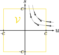
Abbildung 1: Motion of piercing points through a Poincaré section ${\cal P}$ inside a 2-encounter. The box contains stable and unstable coordinates within the ranges $|s|,|u|<c$ corresponding to the volume ${\cal V}$ defined in the text. As ${\cal P}$ is shifted, the unstable components grow and the stable ones shrink, traveling on a hyperbola $\Delta S=su$; arrows denote the direction of motion. At end of the encounter, the piercing points traverse the line $u=c$. Of course, there are also trajectories cutting through the remaining four quadrants of ${\cal V}$.

On the other hand, we can count each trajectory when it leaves the volume ${\cal V}$. Each trajectory finally leaves ${\cal V}$ through one of the $2(l-1)$ faces defined by $u_{J}=\pm c$, $J=1,\ldots,l-1$, with the remaining stable and unstable coordinates restricted to $(-c,c)$. (In contrast trajectories first enter through the faces defined by $s_{J}=\pm c$.) To count trajectories leaving ${\cal V}$ through one of these faces, we consider the current density leading out of ${\cal V}$. We thus multiply the integrand, i.e., the “density” associated to ${\bf x}$, $s$, and $u$, with the velocity of leaving ${\cal V}$. The unstable coordinates change with the velocity $\frac{du_{j}}{dt}=\chi({\bf x})u_{j}$, see Eq. (1). The velocity component perpendicular to the face with $u_{J}=\pm c$ is therefore given by $\chi({\bf x}^{\rm e})c$; here we denoted the corresponding phase-space point by ${\bf x}^{\rm e}$ and fixed the sign such that the velocity of trajectories leaving ${\cal V}$ is taken as positive. The resulting current density has to be integrated over the face of ${\cal V}$ considered, and over time. Dropping proportionality factors arising from the time integral and from probability considerations, we are thus led to Eq. (14), with the Jacobian $\chi({\bf x}^{\rm e})c$ interpreted as a velocity. If the local stretching rate becomes negative, the trajectories can reenter into ${\cal V}$ through the same face, giving a negative contribution to the flux in Eq. (14). However, since each trajectory finally leaves ${\cal V}$, all entries and exits ultimately sum up to yield one positive contribution.

Eqs. (13) and (14) hence represent two equivalent ways of summing over encounters, or trajectories crossing ${\cal V}$. The approach of Eq. (13) is better suited for terms contributing to $K(\tau)$, whereas the approach of Eq. (14), first employed in [24] for Sieber/Richter pairs in two-dimensional systems, yields an easier treatment of the vanishing terms.

Anhang 10.B More than two degrees of freedom

Our results can easily be extended to dynamics with any number $f$ of degrees of freedom. The applicability of the Gutzwiller trace formula to such systems has been extensively studied in [38, 73].

For dynamics with arbitrary $f\geq 2$, the Poincaré section ${\cal P}$ at point ${\bf x}$ is spanned by $f-1$ pairs of stable and unstable directions ${\bf e}^{s}_{m}({\bf x})$, ${\bf e}^{u}_{m}({\bf x})$ ($m=1,2,\ldots,f-1$), as in Eq. (8). The mutual normalization of these directions was fixed in Eq. (9). Each pair of directions comes with separate stretching factors $\Lambda_{m}({\bf x},t)$ and stretching rates $\chi_{m}({\bf x})$, and a separate Lyapunov exponent $\lambda_{m}$.

Our results carry over if we write out the additional index $m$: The piercing points of a given encounter are described by components $\hat{s}_{jm}$, $\hat{u}_{jm}$ ($j=2,\ldots,l$; $m=1,\ldots,f-1)$. Still defining the encounter as the region where all these components are inside $(-c,c)$, the durations of heads and tails, see Eqs. (2-3), generalize to

$$t_{u}=\min_{j,m}\left\{\frac{1}{\lambda_{m}}\ln\frac{c}{|\hat{u}_{jm}|}\right\},\ \ \ \;t_{s}=\min_{j,m}\left\{\frac{1}{\lambda_{m}}\ln\frac{c}{|\hat{s}_{jm}|}\right\}.$$ (15)

The action difference related to one encounter is now given by $\Delta S=\sum_{j,m}s_{jm}u_{jm}$, with $s_{jm},u_{jm}$ defined by the same coordinate transformation as in Subsection 2. The integral over $(L-V)(f-1)$ pairs of stable and unstable components $s_{\alpha jm}$, $u_{\alpha jm}$ in the second line of Eq. (17) yields $(2\pi\hbar)^{(L-V)(f-1)}$, which is just what we need since the Heisenberg time now reads $T_{H}=\frac{\Omega}{(2\pi\hbar)^{f-1}}$.

Given that the encounter ends as soon as one unstable component, say $u_{JM}$, reaches $\pm c$, the $\frac{1}{t_{\rm enc}}$-integral of Appendices 9 and 10.A is split into components $I_{JM}^{\pm}$, with $\lambda$ replaced by $\lambda_{M}$, and $\chi({\bf x})$ by $\chi_{M}({\bf x})$. These components can be evaluated as in case of two degrees of freedom.

Anhang 10.C Summary

We extended our results to general fully chaotic systems with arbitrary number $f$ of degrees of freedom. For inhomogeneously hyperbolic systems, the duration of each encounter not only depends on the differences between piercings, but also on the phase-space location of the first piercing. This dependence had to be taken into account when showing that integrals involving $\frac{1}{t_{\rm enc}}$ effectively vanish. Moreover, we showed explicitly how to implement the necessary average over periodic orbits. Our results carry over to systems with $f>2$ if we write out the additional index $m$, numbering the $f-1$ pairs of stable and unstable directions.

Kapitel 11 Encounter overlap

So far, we have confined ourselves to encounters whose stretches are separated by intervening loops, i.e., do not overlap. To justify this, we now want to show that encounters with overlapping stretches do not give rise to additional orbit pairs, and therefore do not contribute to the form factor. We must distinguish between three special cases. As already mentioned in Section 3, if stretches of two different encounters overlap, these encounters have to be regarded as a single encounter. Generalizing the results of Section 4, we will show that two antiparallel stretches without an intervening loop have to be treated as one single stretch. Finally, we shall see that encounters with overlapping parallel stretches need not be considered because the related partners can also be accessed by reconnections inside non-overlapping encounters.

Anhang 11.A Antiparallel encounter stretches

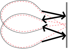
Abbildung 1: Full line: Sketch of an orbit undergoing two almost self-retracing reflections from a hard wall. The encounter depicted by thick full lines could be regarded as a 3-encounter or a 4-encounter with overlapping stretches, or as a 2-encounter with both stretches separated by intervening loops. Dashed line: Partner orbit obtained by reconnecting the four ports of the above encounter.

Two antiparallel encounter stretches can follow each other without an intervening loop only if the encounter involves an almost self-retracing reflection from a hard wall, as in Fig. 4. If the encounter contains more than two stretches, the remaining stretches must be reflected from the same wall; an example, with two almost self-retracing reflections, is depicted in Fig. 1. Note, however, that the almost self-retracing piece in Fig. 4, and each of the two such pieces in Fig. 1, has only two ports. Therefore, the depicted encounters should rather be interpreted in a different way, with each of these pieces viewed as a single stretch, folded back onto itself. The stretches thus defined are separated by loops. Hence, there is no need to consider antiparallel encounters without intervening loops.

Critical readers may wish to check that with this interpretation we do not loose any orbit pairs. For the encounter in Fig. 4, this was already shown in Section 4. Here we want to briefly repeat the main ideas. The encounter in question has only two ports. Since there is no way to reshuffle connections between just two ports, we expect no partner orbit. To check this expectation, we attempt to construct a partner orbit as follows: We place a Poincaré section inside the encounter. The encounter pierces through this section in two phase-space points. Now, we imagine that the orbit is “cut open” in both points and thus split into two parts. These parts have four loose ends. Generalizing the idea of “reconnecting ports”, we can try to reconnect these loose ends. We then obtain an – unphysical – periodic trajectory following one part of the orbit $\gamma$, and the time-reversed of the other part. One might assume that a periodic orbit $\gamma^{\prime}$ can be found by slightly deforming this trajectory. However, by linearizing the equations of motion around the above trajectory, we showed that this suspected partner $\gamma^{\prime}$ coincides with the original orbit $\gamma$. Hence there is no (off-diagonal) partner orbit.

Let us now turn to the encounter in Fig. 1, involving two almost self-retracing reflections. In this example, we can obtain a partner orbit by changing connections between the four ports, like for any 2-encounter; this partner is drawn as a dashed line. We will show that no further partners can be found if we artificially try to interpret the depicted encounter as, say, a 4-encounter. Let us place a Poincaré section ${\cal P}$ somewhere inside the encounter, and cut the orbit open in the four piercing points. A partner orbit $\gamma^{\prime}$ can be found if we reconnect the resulting eight loose ends, and subsequently look for a nearby classical periodic orbit. Using the ideas of Subsection 2, the necessary reconnections can be performed in three successive steps. Each step affects only two piercings, and changes the connections of the corresponding loose ends. We can show that two of these steps effectively do not change the orbit. Let us identify the loose end preceding the upper self-retracing reflection in Fig. 1 with the upper right “port” in Fig. 3. Then, this end is engaged in reconnection steps involving all other loose ends, or “ports”, on the same side. Among these, one step also involves the loose end following the same reflection. This step does not change the orbit, just like reconnections inside the 2-encounter of Fig. 4. The remaining two steps thus suffice to obtain the partner orbit $\gamma^{\prime}$. Repeating the same reasoning for the second reflection, we can show that one further step may be dropped. Hence, one step suffices to obtain the partner orbit, which therefore can be seen as originating from reconnections in a 2-encounter rather than a 4-encounter. We thus see that it suffices to consider the encounter of Fig. 1 as a 2-encounter with both stretches separated by intervening loops, rather than a 4-encounter without intervening loops. Similar arguments apply to encounters involving arbitrarily many almost self-retracing reflections.

Anhang 11.B Antiparallel fringes

Recall that we define an $l$-encounter as a region inside a periodic orbit in which $l$ orbit stretches come close up to time reversal. Attached to the sides of the encounter are “fringes” in which only some of the $l$ stretches remain close while others have already gone astray, as shown in Fig. 2a. We shall now demonstrate that these fringes do not affect the spectral form factor.

As a first example, let us assume that two antiparallel stretches remain close after the end of the encounter, as in Fig. 2a. If there is no intervening loop, the orbit has to undergo an almost self-retracing reflection (see Fig. 2b). No connections can be switched between the two stretches involved. Thus, we cannot build a partner orbit in which all three stretches of the encounter are changed. Of course, we can reshuffle connections between, e.g., the upper and lower stretches in Fig. 2b, without changing the connections of the middle stretch. The arising partner is, however, associated to a 2-encounter rather than a 3-encounter. Hence, the 3-encounter in Fig. 2b has to be disregarded. The same arguments apply to any encounter in which two antiparallel “fringe” stretches follow each other without an intervening loop. (Note that the results in the end of Appendix 11.A carry over to fringes as well.)

On the other hand, if the “fringe” stretches are separated by an external loop, a partner orbit can be obtained as usual, by reshuffling connections between all stretches of the encounter, see Fig. 2a. To make sure there is an intervening loop, we impose minimal separations between piercing points, similar to those used for excluding overlap between encounters in Section 4. Consider two subsequent antiparallel stretches, say, a stretch $j$ leading from left to right, and a stretch $j+1$ leading from right to left. After these stretches have pierced through a Poincaré section ${\cal P}$ with unstable coordinates $\hat{u}_{\alpha j}$ and $\hat{u}_{\alpha,j+1}$, they will remain close for a time $\frac{1}{\lambda}\ln\frac{c}{|\hat{u}_{\alpha j}-\hat{u}_{\alpha,j+1}|}$. This duration contains both the time $t_{u}$ till the end of the $\alpha$-th encounter, see Eq. (2), and an additional time span after the end of the encounter, which gives the duration of the fringe. Using the unstable coordinates $\hat{u}_{\alpha j}^{\rm e}$ of piercing through a section in the end of the encounter (depending on $\hat{u}_{\alpha j}$ via $\hat{u}_{\alpha j}^{\rm e}=\hat{u}_{\alpha j}{\rm e}^{\lambda t_{u}}$), this additional time may be written as $\frac{1}{\lambda}\ln\frac{c}{|\hat{u}_{\alpha j}^{\rm e}-\hat{u}_{\alpha,j+1}^{\rm e}|}$. Hence, the minimal time difference $2t_{u}$ between piercings demanded in Section 4 has to be incremented by a time $\frac{2}{\lambda}\ln\frac{c}{|\hat{u}_{\alpha j}^{\rm e}-\hat{u}_{\alpha,j+1}^{\rm e}|}$, depending on the unstable coordinates only via $\hat{u}^{\rm e}$ or, equivalently, via coordinates $u^{\rm e}$ defined through a coordinate transformation as in Subsection 2.

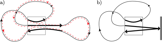
Abbildung 2: 3-encounter (in the box) with a “fringe” where only two antiparallel stretches remain close. Stretches are separated by a loop in a) but not in b); an almost self-retracing reflection arises in the latter case. A partner orbit reconnecting the ports of all three stretches (dashed line) is obtained only in case a).

Similarly, if the $j$-th stretch points from right to left and the $(j+1)$-st stretch points from left to right, the corresponding minimal distance has to be incremented by an amount purely depending on the stable coordinates $s^{\rm b}$ in the beginning of the encounter. The contribution of each encounter to the total sum of minimal separations can therefore be written in the form

$$t_{\rm excl}^{\alpha}=l_{\alpha}t_{\rm enc}^{\alpha}+\Delta t_{s}^{\alpha}(s^{{\rm b}})+\Delta t_{u}^{\alpha}(u^{{\rm e}})$$ (1)

with $\Delta t_{s}$ and $\Delta t_{u}$ functions of $s^{\rm b}$ and $u^{\rm e}$ only; the precise form of these functions will not be needed in the following. The numerator in the density of phase-space separations $w_{T}(s,u)$, Eq. (10), has to be modified accordingly; each $l_{\alpha}t_{\rm enc}^{\alpha}$ is replaced by $t_{\rm excl}^{\alpha}$.

We proceed to show that the summands $\Delta t_{s}^{\alpha}$ and $\Delta t_{u}^{\alpha}$ do not affect the spectral form factor. By reasoning as in Subsection 5, we see that only those terms of the multinomial expansion of the numerator in $w_{T}(s,u)$ contribute to $K(\tau)$ which involve a product of all $t_{\rm excl}^{\alpha}$. Due to $t_{\rm excl}^{\alpha}\neq l_{\alpha}t_{\rm enc}^{\alpha}$, these terms now have to be written as (compare Eq. (5))

$$\frac{w_{T}^{\rm contr}(s,u)}{L} = h(\vec{v})\left(\frac{T}{\Omega}\right)^{L-V}\prod_{\alpha}\frac{t_{\rm excl}^{\alpha}}{l_{\alpha}t_{\rm enc}^{\alpha}}$$ (2)

$$= h(\vec{v})\left(\frac{T}{\Omega}\right)^{L-V}\prod_{\alpha}\left[1+\frac{\Delta t_{s}^{\alpha}+\Delta t_{u}^{\alpha}}{l_{\alpha}t_{\rm enc}^{\alpha}}\right],$$

and contribute to the form factor as (compare Eq. (17))

$$\kappa\tau h(\vec{v})\left(\frac{T}{\Omega}\right)^{L-V}\prod_{\alpha}\left[\int d^{L-V}s\,d^{L-V}u\left(1+\frac{\Delta t_{s}^{\alpha}+\Delta t_{u}^{\alpha}}{l_{\alpha}t_{\rm enc}^{\alpha}}\right){\rm e}^{\frac{\rm i}{\hbar}\sum_{j}s_{\alpha j}u_{\alpha j}}\right].$$ (3)

The integral in Eq. (3) coincides with the one in Eq. (17) up to the fringe corrections $\propto\frac{\Delta t_{s}^{\alpha}}{t_{\rm enc}^{\alpha}}$ and $\propto\frac{\Delta t_{u}^{\alpha}}{t_{\rm enc}^{\alpha}}$. By reasoning similarly as in Appendix 9, one easily shows that the resulting integrals vanish in the semiclassical limit: When integrating over $\frac{\Delta t_{u}}{t_{\rm enc}^{\alpha}}$, the additional factor $\Delta t_{u}^{\alpha}(u^{\rm e})$ affects only the integral over $u^{\rm e}$ inside Eq. (2), whereas the rapidly oscillating integral over $s_{J}^{\rm e}$ remains unchanged. For $\frac{\Delta t_{s}^{\alpha}}{t_{\rm enc}^{\alpha}}$ we have to consider a surface of section in the beginning rather than in the end of the encounter. Then, the integral over the unstable coordinate $u_{J^{\prime}}^{\rm b}$ associated to the largest stable coordinate $s_{J^{\prime}}^{\rm b}=\pm c$ oscillates rapidly as $\hbar\to 0$; this integral remains unaffected by the factor $\Delta t_{s}(s^{\rm b})$. For antiparallel orbit stretches, fringe corrections to the form factor are hence revealed as negligible in the semiclassical limit.

The present treatment can immediately be generalized to $f>2$, if we write out the additional index $m$, and to inhomogeneously hyperbolic systems, if we allow $t_{\rm enc}$ to depend on ${\bf x}$. In the latter case, $\Delta t_{s}$ will be a function of both $s^{\rm b}$ and the phase-space points ${\bf x}^{\rm b}$ in the beginning of the encounter, and $\Delta t_{u}$ will depend on $u^{\rm e}$ and ${\bf x}^{\rm e}$ in the end of the encounter.

Anhang 11.C Parallel encounter stretches

We now turn to parallel encounter stretches. We shall see that if two subsequent parallel stretches of an encounter overlap or follow each other after a relatively short loop, the encounter will have a very peculiar structure.

Whenever two points of a periodic orbit $\gamma$ are close in phase space, the orbit part between these points must be almost periodic – and hence in the vicinity of a shorter periodic orbit $\tilde{\gamma}$. The two phase-space points belong to mutually close encounter stretches, which thus are near to $\tilde{\gamma}$ as well. Typically, these stretches are short compared to the intervening loop. Hence $\gamma$ follows only slightly more than one revolution of $\tilde{\gamma}$ (Fig. 3a).

In contrast, if the stretches are only separated by a short loop (see Fig. 3b), the orbit $\gamma$ will remain close to $\tilde{\gamma}$ for almost two periods: Each of the two stretches follows nearly one period of $\tilde{\gamma}$, and the short intervening loop, too, remains in the vicinity of $\tilde{\gamma}$.

Finally, if the stretches overlap, $\gamma$ will contain two or more repetitions of $\tilde{\gamma}$; see Fig. 3c for an example of $\gamma$ following slightly more than two periods of $\tilde{\gamma}$.

All further stretches of the encounters considered also have to come close to $\tilde{\gamma}$. The orbit $\gamma$ will thus approach $\tilde{\gamma}$ several times, and in case of overlap or near-overlap of stretches at least one approach lasts significantly longer than one revolution of $\tilde{\gamma}$.

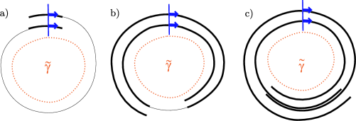
Abbildung 3: Two parallel encounter stretches (thick lines) a) separated by a comparatively long loop (thin line), b) separated by a short loop, c) overlapping in a region depicted by two very close thick lines. The long orbit respectively follows a) slightly more than one, b) slightly less than two, c) more than two periods of the shorter orbit $\tilde{\gamma}$ (dotted line). Also depicted are Poincaré sections approximately in the center of the encounters, each with two piercing points.

We must now look for partner orbits related to such encounters. To do so, we shall follow the procedure outlined in Appendix 11.A: We place a Poincaré section ${\cal P}$ somewhere inside the encounter, and imagine the orbit $\gamma$ cut into parts in its points of piercing through ${\cal P}$. We then change connections between the loose ends of these parts, and slightly deform the resulting closed trajectory to obtain a classical periodic orbit.

The crucial point is now the following: If $\gamma$ follows nearly two, or even several, revolutions close to $\tilde{\gamma}$, we have large freedom in selecting piercing points. For example, the encounter of Fig. 4c contains a region with three mutually close lines, corresponding to only two encounter stretches. Placing a Poincaré section inside this region, we find three piercing points. We need to select two of them. If the encounter contains further stretches, these stretches will also pierce through our section, possibly several times, and we have to select one piercing for each stretch. Some of the possible choices of piercings formally correspond to different encounters, even though they yield the same partner orbit. Therefore blindly considering all encounters and associating with each of them a partner orbit we would count certain orbit pairs several times.

In the following, we shall identify the conditions under which piercing points of different encounters yield the same partner. We will demonstrate that within each family of encounters related to the same partner, only for one member the stretches are separated by loops exceeding certain minimal durations. When evaluating the form factor, we will include only this representative encounter and disregard all other members of the family, to avoid overcounting of orbit pairs. The resulting contribution to the form factor will turn out the same as if we only demand the intervening loops to be positive; this is why the latter condition was used in the main part.

1 Parallel 3-encounters

We first focus on the example of a parallel 3-encounter inside an orbit $\gamma$. The stretches of this encounter pierce through a Poincaré section ${\cal P}$ in phase-space points ${\bf x}_{1}$, ${\bf x}_{2}$, and ${\bf x}_{3}$, see Fig. 4a. We shall derive a restriction on the time difference $t_{12}$ between ${\bf x}_{1}$ and ${\bf x}_{2}$. Since ${\bf x}_{1}$ and ${\bf x}_{2}$ are close in phase space, the part of $\gamma$ between these points approximately follows a periodic orbit $\tilde{\gamma}$ with period close to $t_{12}$. The orbit $\gamma$ will also stay close to $\tilde{\gamma}$ for some time before ${\bf x}_{1}$ and after ${\bf x}_{2}$. The whole region close to $\tilde{\gamma}$ is drawn as a thick full line in Fig. 4a. In the vicinity of ${\bf x}_{3}$, the orbit $\gamma$ has to approach $\tilde{\gamma}$ for a second time. This second approach is represented by a dash-dotted line.

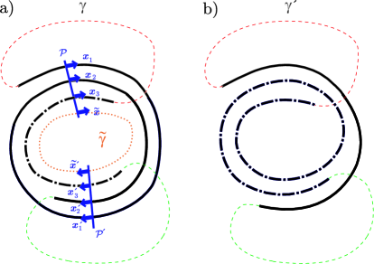
Abbildung 4: a) An orbit $\gamma$ approaches a shorter orbit $\tilde{\gamma}$ (dotted line) in two regions (marked by thick full and dash-dotted lines). It pierces three times through each of the Poincaré sections ${\cal P}$ and ${\cal P}^{\prime}$; the two sets of piercings belong to two different encounters. b) Reconnections in either encounter lead to the same partner $\gamma^{\prime}$, with one revolution of $\tilde{\gamma}$ transposed between the full and dash-dotted regions.

The piercings ${\bf x}_{1}$, ${\bf x}_{2}$, and ${\bf x}_{3}$ cut $\gamma$ into three parts. When reconnecting the “loose ends” of these parts to form a partner orbit, we change the ordering of orbit parts. This reordering may be interpreted as cutting out the orbit part leading from ${\bf x}_{1}$ to ${\bf x}_{2}$ (close to $\tilde{\gamma}$) and reinserting it between the two other parts, i.e., when $\gamma$ traverses ${\bf x}_{3}$. In other words, one revolution of $\tilde{\gamma}$ is transposed between the two regions approaching $\tilde{\gamma}$. The resulting partner is shown in Fig. 4b, with one revolution of $\tilde{\gamma}$ taken out from the region depicted by the thick full line and reinserted inside the dash-dotted region. (Recall that after transposing orbit parts the resulting trajectory must be slightly deformed to yield a classical periodic orbit.)

Crucially, different sets of piercing points may yield the same partner. We have already seen that the Poincaré section may be moved continuously through the encounter. The piercing points will then all be shifted by the same amount of time. All sets of piercings thus obtained belong to the same encounter and yield the same partner.

In the present scenario, the freedom in choosing piercing points is even larger. To show this, let us compare two sets of piercings, the above points ${\bf x}_{1}$, ${\bf x}_{2}$, ${\bf x}_{3}$ in a Poincaré section ${\cal P}$, and piercings ${\bf x}_{1}^{\prime}$, ${\bf x}_{2}^{\prime}$, ${\bf x}_{3}^{\prime}$ in a (possibly) different Poincaré section ${\cal P}^{\prime}$. We assume that the new piercings are also close to $\tilde{\gamma}$, with ${\bf x}_{1}^{\prime}$ and ${\bf x}_{2}^{\prime}$ inside the same region of approach to $\tilde{\gamma}$ as ${\bf x}_{1}$ and ${\bf x}_{2}$, and ${\bf x}_{3}^{\prime}$ in the same region as ${\bf x}_{3}$, as in Fig. 4a. Furthermore, we demand that the points ${\bf x}_{1}^{\prime}$ and ${\bf x}_{2}^{\prime}$ enclose one revolution of $\tilde{\gamma}$, just like ${\bf x}_{1}$ and ${\bf x}_{2}$. Then, upon reconnection again one revolution of $\tilde{\gamma}$ (the piece leading from ${\bf x}_{1}^{\prime}$ to ${\bf x}_{2}^{\prime}$) is cut out from the first region approaching $\tilde{\gamma}$ and reinserted inside the second region of approach (at position ${\bf x}_{3}^{\prime}$). Hence we obtain the same partner as for the “old” piercings.

The phase-space points ${\bf x}_{1}^{\prime}$, ${\bf x}_{2}^{\prime}$, ${\bf x}_{3}^{\prime}$ will typically be shifted along the orbit compared to their counterparts ${\bf x}_{1}$, ${\bf x}_{2}$, ${\bf x}_{3}$. The first two points must both be shifted by the same amount of time $t_{A}$, to guarantee that they remain separated by one period of $\tilde{\gamma}$. The third one may be shifted by a different time $t_{B}$. After these shifts, all phase-space points must meet inside the same Poincaré section ${\cal P}^{\prime}$, such that the orbit $\gamma$ pierces through ${\cal P}^{\prime}$ in ${\bf x}_{1}^{\prime}$, ${\bf x}_{2}^{\prime}$, and ${\bf x}_{3}^{\prime}$.

We have seen that for $t_{A}=t_{B}$, i.e., if all points are shifted by the same amount of time, the piercings ${\bf x}_{1}^{\prime}$, ${\bf x}_{2}^{\prime}$, and ${\bf x}_{3}^{\prime}$ form part of the same encounter as ${\bf x}_{1}$, ${\bf x}_{2}$, and ${\bf x}_{3}$, crossed by a different Poincaré section. However, if $t_{A}\neq t_{B}$ our “new” piercings belong to a different encounter than the “old” ones, with both encounters yielding the same partner orbit. In the example of Fig. 4a, the points ${\bf x}_{1}^{\prime}$ and ${\bf x}_{2}^{\prime}$ are shifted to the future ($t_{A}>0$) compared to their counterparts ${\bf x}_{1}$ and ${\bf x}_{2}$, whereas ${\bf x}_{3}^{\prime}$ is located to the past of ${\bf x}_{3}$ ($t_{B}<0$). Nevertheless, both sets of piercing points give rise to the partner orbit depicted in Fig. 4b, with one revolution of $\tilde{\gamma}$ transposed between the two regions approaching $\tilde{\gamma}$.

Not all encounters allow for such alternative piercings. Roughly speaking, to find alternative piercings with $t_{A}>0$ and $t_{B}<0$, the orbit $\gamma$ must follow $\tilde{\gamma}$ long enough such that points shifted in two opposite directions can meet again in the same Poincaré section ${\cal P}^{\prime}$. There is a chance for such piercing points to exist if the encounter stretches overlap or are separated by short loops, and therefore $\gamma$ follows several periods of $\tilde{\gamma}$. We proceed to determine the precise conditions.

First of all, how far can the points be shifted without leaving the vicinity of $\tilde{\gamma}$? To answer this question, we need to determine the stable and unstable coordinates of the phase-space point $\tilde{{\bf x}}$ in which the orbit $\tilde{\gamma}$ intersects the section ${\cal P}$. The trajectories passing through $\tilde{{\bf x}}$ and ${\bf x}_{1}$ remain close at least for one period of $\tilde{\gamma}$ after which they are carried to $\tilde{{\bf x}}$ and ${\bf x}_{2}$, respectively. Thus by reasoning similarly as in Subsection 2 we see that $\tilde{{\bf x}}$ and ${\bf x}_{1}$ have approximately the same unstable component $\hat{\tilde{u}}\approx\hat{u}_{1}=0$.

Likewise the trajectories passing through $\tilde{{\bf x}}$ and ${\bf x}_{2}$ remain close for large negative times, such that the stable component of $\tilde{{\bf x}}$ may be approximated by $\hat{\tilde{s}}\approx\hat{s}_{2}$.

The first two phase-space points may be shifted to the future as long as both remain close to $\tilde{\gamma}$. The second point starts to deviate significantly from $\tilde{\gamma}$ earlier than the first one. Therefore, we can shift both phase-space points until the unstable separation between ${\bf x}_{2}$ and $\tilde{{\bf x}}$, i.e., $\hat{u}_{2}-\hat{\tilde{u}}\approx\hat{u}_{2}-\hat{u}_{1}$, grows beyond our bound $c$. This will happen after a time $\frac{1}{\lambda}\ln\frac{c}{|\hat{u}_{2}-\hat{u}_{1}|}$. We will thus stay in the vicinity of $\tilde{\gamma}$ while

$$t_{A}<\frac{1}{\lambda}\ln\frac{c}{|\hat{u}_{2}-\hat{u}_{1}|}.$$ (4)

The third point may be shifted to the past as long as the stable component of its separation from $\tilde{\gamma}$, i.e., $\hat{s}_{3}-\hat{\tilde{s}}\approx\hat{s}_{3}-\hat{s}_{2}$ remains below $c$; this leads to the restriction

$$-t_{B}<\frac{1}{\lambda}\ln\frac{c}{|\hat{s}_{3}-\hat{s}_{2}|}.$$ (5)

The shifted points ${\bf x}_{1}^{\prime}$, ${\bf x}_{2}^{\prime}$, and ${\bf x}_{3}^{\prime}$ allow for reconnections only if they meet inside the same Poincaré section ${\cal P}^{\prime}$. This restriction is trivially fulfilled if all phase-space points are shifted by the same amount of time $t_{A}=t_{B}$ from one section ${\cal P}$ to a different section ${\cal P}^{\prime}$. Likewise, the points will meet inside the same section if, say, ${\bf x}_{1}$ and ${\bf x}_{2}$ effectively perform one more rotation around $\tilde{\gamma}$ than ${\bf x}_{3}$. After one such rotation, ${\bf x}_{1}$ and ${\bf x}_{2}$ end up in the same Poincaré section as they started from. More generally, the shifted points will meet in the same Poincaré section if ${\bf x}_{1}$ and ${\bf x}_{2}$ perform an integer number of rotations more, or less, than ${\bf x}_{3}$. This means that the time difference $t_{A}-t_{B}$ must involve an integer number of periods of $\tilde{\gamma}$, i.e., an integer multiple of $t_{12}$. The restriction of having ${\bf x}_{1}^{\prime}$, ${\bf x}_{2}^{\prime}$, and ${\bf x}_{3}^{\prime}$ located inside the same Poincaré section thus boils down to

$$t_{A}-t_{B}=n\,t_{12}$$ (6)

with $n=-2,-1,0,1,2,\ldots$. If we restrict ourselves to $t_{A}>0$, $t_{B}<0$, we must have positive $n=1,2,\ldots$. Combining Eqs. (4-6), we are led to

$$n\,t_{12}<\frac{1}{\lambda}\ln\frac{c}{|\hat{u}_{2}-\hat{u}_{1}|}+\frac{1}{\lambda}\ln\frac{c}{|\hat{s}_{3}-\hat{s}_{2}|}\,.$$ (7)

If the separation $t_{12}$ is sufficiently large, i.e., if

$$t_{12}>\frac{1}{\lambda}\ln\frac{c}{|\hat{u}_{2}-\hat{u}_{1}|}+\frac{1}{\lambda}\ln\frac{c}{|\hat{s}_{3}-\hat{s}_{2}|}\,,$$ (8)

Eq. (7) has no positive solution $n$. In this case, no alternative encounter can be obtained by shifting the first two phase-space points to the future and the third one to the past; otherwise such encounters can be found, one for each possible $n\geq 1$. For the case $t_{A}<0$, $t_{B}>0$, analogous reasoning yields a similar condition.

We are now prepared to single out one representative encounter for each orbit pair. Inside each family of equivalent encounters we take the member for which the time between piercings ${\bf x}_{2}$ and ${\bf x}_{3}$ is smallest. This time difference is decreased by all shifts with $t_{A}>0$, $t_{B}<0$, and increased if $t_{A}<0$, $t_{B}>0$. ($t_{A}$ and $t_{B}$ with equal sign need not be considered since we may shift ${\cal P}^{\prime}$ until the signs are opposite.) Hence from the chosen encounter no alternative one may be accessible through a shift with $t_{A}>0$, $t_{B}<0$. Consequently our representative encounter has to satisfy Eq. (8). Using the stable coordinates $\hat{s}_{j}^{\rm b}=\hat{s}_{j}{\rm e}^{\lambda t_{s}}$ in the beginning of the encounter and the unstable coordinates $\hat{u}_{j}^{\rm e}=\hat{u}_{j}{\rm e}^{\lambda t_{u}}$ in the end, and recalling that $t_{\rm enc}=t_{s}+t_{u}$, we may rewrite this condition as

$$t_{12}>t_{\rm enc}+\frac{1}{\lambda}\ln\frac{c}{|\hat{u}_{2}^{\rm e}-\hat{u}_{1}^{\rm e}|}+\frac{1}{\lambda}\ln\frac{c}{|\hat{s}_{3}^{\rm b}-\hat{s}_{2}^{\rm b}|}\,.$$ (9)

Minimal separations between, say, the second and third piercing, are obtained from Eq. (9) by cyclic permutation.

Eq. (9) can be interpreted as follows: Demanding $t_{12}>t_{\rm enc}$ implies that we consider only encounters whose stretches do not overlap, as postulated in the main part. The additional increment in Eq. (9) can be regarded as a minimal loop duration. If the loop in between the encounter stretches is very large, $\gamma$ will follow $\tilde{\gamma}$ for only slightly more than one period and there will be no alternative encounter. If the loop slightly exceeds our threshold, there typically are alternative encounters, but the one considered is the encounter representative for our orbit pair. The boundary between both scenarios is irrelevant for our considerations.

The minimal loop duration depends purely on $\hat{s}^{\rm b}$ and $\hat{u}^{\rm e}$. In the language of Appendix 11.B, the second summand in Eq. (9) gives the duration of the “fringe” where the first two stretches remain close after the end of the encounter; likewise the third summand represents the duration of the fringe where the second and third stretch come close before the beginning of the encounter.

Due to the exclusive dependence on $\hat{s}^{\rm b}$ and $\hat{u}^{\rm e}$, respectively, the additional summands in Eq. (9) do not affect the form factor in the semiclassical limit. Again the sum of minimal time differences is of the same form, Eq. (1), as met in case of antiparallel fringes, and the reasoning of Appendix 11.B carries over accordingly.

Focusing on the example of a parallel 3-encounter, we have thus justified the treatment in the main part: We have shown that encounters with overlapping stretches must be excluded, and that corrections due to the exclusion of encounter stretches separated by short loops do not affect $K(\tau)$ in the semiclassical limit.

2 General $l$-encounters

The previous line of reasoning may be generalized to $l$-encounters with arbitrary $l$. For simplicity, we first consider orbit pairs $(\gamma,\gamma^{\prime})$ differing in one encounter with all $l$ stretches almost parallel. This encounter pierces $l$ times through a Poincaré section ${\cal P}$, cutting the orbit $\gamma$ into $l$ parts. We label each of the $l$ orbit parts by the same number as the following piercing point; this label coincides with the number of the loop and the entrance port included in the corresponding part. As before, the second orbit part, between the first two piercing points, is close to a shorter periodic orbit $\tilde{\gamma}$. We shall see that the partner $\gamma^{\prime}$ can be obtained by performing reconnections inside two separate sets of piercing points, and afterwards cutting out the part close to $\tilde{\gamma}$ and reinserting it in a different place. In analogy to the preceding Subsection, the two sets of points may be shifted independently, without changing the partner orbit $\gamma^{\prime}$.

We will again employ methods of permutation theory. The order of orbit parts in $\gamma$ is given by the permutation $P^{\gamma}=P_{\rm loop}=(1,2,\ldots,l)$. In the partner orbit $\gamma^{\prime}$, the $l$ parts are ordered differently. This ordering is described by a permutation $P\neq P^{\gamma}$. The permutation $P$ also determines the encounter permutation $P_{\rm enc}=P_{\rm loop}^{-1}P$, giving the connections between ports, or loose ends, inside $\gamma^{\prime}$. For orbit pairs differing in one $l$-encounter, $P_{\rm enc}$ has a single cycle of length $l$.

We can proceed from $\gamma$ to $\gamma^{\prime}$ in two steps. In the first step, we go from $\gamma$ to an intermediate orbit $\gamma_{\rm int}$. This orbit has the parts $1,3,4,\ldots,l$ ordered as in $\gamma^{\prime}$, but the second orbit part still follows the first. When reordering the orbit parts, the first piercing point, on the border between the first and the second orbit part, remains practically unaffected. All other piercing points are changed. To describe $\gamma_{\rm int}$ in terms of permutations, it is technically easier to consider the first two orbit parts as one single part, labelled by the index 1. (Treating the first two orbit parts as one means that the first piercing point, unchanged in $\gamma_{\rm int}$, is disregarded, and that the second piercing point, following the two initial orbit parts, is renamed into the first.) The ordering of orbit parts in $\gamma_{\rm int}$ is then given by a permutation $Q$ obtained from the permutation $P$, describing $\gamma^{\prime}$, by leaving out the label 2. Likewise, we have to eliminate the element 2 from the permutation $P_{\rm loop}$, leading to a new permutation $Q_{\rm loop}$. The intra-encounter connections of $\gamma_{\rm int}$ are thus described by the permutation $Q_{\rm enc}=Q_{\rm loop}^{-1}Q$. The cycle structure of $Q_{\rm enc}$ was already investigated in Subsection 3, where for formal reasons we eliminated $L=l$ rather than $2$; all our results carry over if we eliminate 2 instead. We have seen that inside $Q_{\rm enc}$, the $l$-cycle of $P_{\rm enc}$ is split in two cycles, given in Eq. (9). Hence, $\gamma_{\rm int}$ may be obtained from $\gamma$ by independent reconnections inside two separate sets of encounter stretches.

In the second step, we go from $\gamma_{\rm int}$ to the partner $\gamma^{\prime}$. We thus have to cut out the second orbit part, close to $\tilde{\gamma}$, and reinsert it into its destined place.

We are now prepared to generalize the arguments of the previous Subsection. The $l$ piercing points can be divided in two sets $A$ and $B$, corresponding to the two cycles of $Q_{\rm enc}$; the first piercing point, not taking part in reconnections, must be included in the same set $A$ as the second one. We can now show that the same partner $\gamma^{\prime}$ arises if the points of $A$ and $B$ are shifted independently by respective times $t_{A}$ and $t_{B}$ (e.g., $t_{A}>0$ and $t_{B}<0$), provided that all piercings remain in the vicinity of $\tilde{\gamma}$ and end up inside the same Poincaré section ${\cal P}^{\prime}$. First, note that reconnections inside $A$ yield the same result as before, since the phase-space points of $A$ were all shifted by an equal amount of time and stayed mutually close. Similar arguments apply to the reconnections inside $B$. Next, we transpose the orbit part enclosed between the first two piercings. This part still contains one revolution of $\tilde{\gamma}$, given that the first and second point were shifted by the same time $t_{A}$ and remained in the vicinity of $\tilde{\gamma}$. Hence, for both the “old” and the “new” piercings, one revolution of $\tilde{\gamma}$ is cut out from the same region approaching $\tilde{\gamma}$, and reinserted inside a different region. Consequently, in both cases we obtain the same $\gamma^{\prime}$.

To guarantee that all points of $A$ remain near $\tilde{\gamma}$, Eq. (4) must be replaced by

$$t_{A}<\frac{1}{\lambda}\ln\frac{c}{\max_{j\in A}|\hat{u}_{1}-\hat{u}_{j}|}\,.$$ (10)

Similarly, the points included in $B$ will stay in the vicinity of $\tilde{\gamma}$ if

$$-t_{B}<\frac{1}{\lambda}\ln\frac{c}{\max_{j\in B}|\hat{s}_{2}-\hat{s}_{j}|}\,.$$ (11)

As above, we choose a representative encounter from which no other encounter is accessible through a shift with $t_{A}>0$ and $t_{B}<0$. The piercing points of this representative encounter now have to satisfy the restriction

$$t_{12}>t_{\rm enc}+\frac{1}{\lambda}\ln\frac{c}{\max_{j\in A}|\hat{u}^{\rm e}_{1}-\hat{u}^{\rm e}_{j}|}+\frac{1}{\lambda}\ln\frac{c}{\max_{j\in B}|\hat{s}^{\rm b}_{2}-\hat{s}^{\rm b}_{j}|}\,,$$ (12)

generalizing Eq. (9). Again, the form factor remains unaffected by the increment depending purely on $\hat{s}^{\rm e}$ and $\hat{u}^{\rm e}$.

Our results directly carry over to orbit pairs differing in several parallel encounters, and can be further generalized to time-reversal invariant systems. In the latter case, some of the remaining piercing points may be approximately time-reversed with respect to ${\bf x}_{1}$ and ${\bf x}_{2}$. Such time-reversed points need to be shifted by an amount of time $-t_{A}$ or $-t_{B}$ rather than $t_{A}$ or $t_{B}$, to make sure that all points are moved into the same direction. Moreover, our reasoning extends to $f>2$ and inhomogeneous hyperbolicity as outlined in the antiparallel case.

3 Symbolic dynamics

We would like to illustrate the above results by a simple example, elucidating their relation to symbolic dynamics. We consider a parallel 3-encounter, with two overlapping stretches and – in contrast to the preceding Subsections – no fringes attached. In symbolic dynamics, all three encounter stretches will then be characterized by the same sequence ${\cal E}$. Whenever two subsequent stretches overlap, so do the corresponding symbol sequences. This is only possible if ${\cal E}$ has a special structure. The simplest symbol sequences allowing for such overlap are of the form ${\cal E}={\cal X}{\cal Y}{\cal X}$ with ${\cal X}$ and ${\cal Y}$ arbitrary subsequences. The latter structure permits two subsequent strings ${\cal E}$ to overlap in ${\cal X}$ and merge to a symbol sequence ${\cal X}{\cal Y}{\cal X}{\cal Y}{\cal X}$, the middle ${\cal X}$ denoting the overlapping piece. The form ${\cal E}={\cal X}{\cal Y}{\cal X}$ obviously limits the length of the overlap ${\cal X}$ to less than half the length of ${\cal E}$.

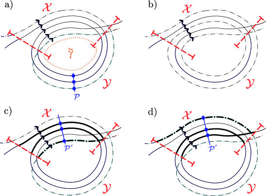
Abbildung 5: Overlap of parallel encounter stretches: a) An orbit $\gamma$ twice approaches a shorter orbit $\tilde{\gamma}={\cal X}{\cal Y}$ (dotted line); the approaches, depicted by thick full and dash-dotted lines, have symbol sequences ${\cal X}{\cal Y}{\cal X}{\cal Y}{\cal X}$ and ${\cal X}{\cal Y}{\cal X}$. Also depicted is a Poincaré section ${\cal P}$ inside the region ${\cal Y}$, with three piercings. b) The partner $\gamma^{\prime}$ has one repetition of $\tilde{\gamma}$ shifted between the two regions. c), d) Two shorter 3-encounters (named (i) and (ii) in the text) can be found in the region ${\cal X}$. They are depicted by thick lines and pierce three times through a Poincaré section ${\cal P^{\prime}}$ inside ${\cal X}$. The three encounters depicted in a), c), and d) all yield the same partner b). The encounter in d) is chosen as a representative encounter: Starting from this representative, no alternative encounter can be found if we shift the piercing points of the thick full stretches to the future, and the one of the thick dash-dotted stretch to the past.

The orbit $\gamma$ now contains two regions approaching a shorter orbit $\tilde{\gamma}$ with symbol sequence ${\cal X}{\cal Y}$: one region with the sequence ${\cal X}{\cal Y}{\cal X}{\cal Y}{\cal X}$ formed out of the merger of two stretches, and one region with a sequence ${\cal X}{\cal Y}{\cal X}$ consisting of the remaining third stretch. If we denote the two intervening loops by ${\cal L}_{1}$ and ${\cal L}_{2}$, $\gamma$ will have the symbol string

$$\gamma=({\cal X}{\cal Y}{\cal X}{\cal Y}{\cal X}){\cal L}_{1}({\cal X}{\cal Y}{\cal X}){\cal L}_{2}\,.$$ (13)

This scenario is illustrated in Fig. 5a. Two Poincaré sections, represented by dashed lines, divide the shorter orbit $\tilde{\gamma}$ in two pieces, with corresponding symbol sequences ${\cal X}$ and ${\cal Y}$. The longer orbit $\gamma$ approaches $\tilde{\gamma}$ twice. The first approach, depicted by a full line, contains two full revolutions of $\tilde{\gamma}={\cal X}{\cal Y}$, and one additional piece close to the segment with symbol sequence ${\cal X}$ (not shown in the picture). After a loop with sequence ${\cal L}_{1}$, $\gamma$ remains close to $\tilde{\gamma}$ for one full revolution of $\tilde{\gamma}$, and one additional piece with the symbol sequence ${\cal X}$. This second approach is represented by a dash-dotted line. The orbit $\tilde{\gamma}$ finally closes itself after an additional loop with the sequence ${\cal L}_{2}$ (again not depicted).

As shown previously, the partner orbit $\gamma^{\prime}$ has one revolution of $\tilde{\gamma}={\cal X}{\cal Y}$ transposed between the two regions close to $\tilde{\gamma}$; see Fig. 5b. In symbolic dynamics, it is therefore characterized by

$$\gamma^{\prime}=({\cal X}{\cal Y}{\cal X}){\cal L}_{1}({\cal X}{\cal Y}{\cal X}{\cal Y}{\cal X}){\cal L}_{2}\,.$$ (14)

If we place a Poincaré section ${\cal P}$ inside the region with symbol sequence ${\cal Y}$, the orbit $\gamma$ will pierce through this section in three phase-space points. The latter section may be shifted freely through the encounter. The piercing points are then all shifted by the same amount of time, either to the preceding or to the following pieces with symbol sequences ${\cal X}$. All these sets of piercings correspond to the same encounter and lead to the same partner orbit.

We have already seen that there is even more freedom in choosing piercing points: The two points inside the region ${\cal X}{\cal Y}{\cal X}{\cal Y}{\cal X}$ and the point inside ${\cal X}{\cal Y}{\cal X}$ may be shifted independently, as long as they remain inside these regions and end up inside the same Poincaré section ${\cal P}^{\prime}$; recall that the two points inside ${\cal X}{\cal Y}{\cal X}{\cal Y}{\cal X}$ must both be shifted by the same amount of time. This gives two additional possibilities:

1. The piercing points of ${\cal X}{\cal Y}{\cal X}{\cal Y}{\cal X}$ may be shifted to the past, whereas the piercing of ${\cal X}{\cal Y}{\cal X}$ is shifted to the future. The shifted points are placed inside the first and second ${\cal X}$ of ${\cal X}{\cal Y}{\cal X}{\cal Y}{\cal X}$, and inside the final ${\cal X}$ in ${\cal X}{\cal Y}{\cal X}$.

2. Alternatively, the points of ${\cal X}{\cal Y}{\cal X}{\cal Y}{\cal X}$ may be shifted to the future, i.e., to the second and third ${\cal X}$, whereas the point inside ${\cal X}{\cal Y}{\cal X}$ is shifted to the past, i.e., to the first ${\cal X}$.

In both cases, the phase-space points have to be shifted until they meet in the same Poincaré section ${\cal P}^{\prime}$. The two additional possibilities are depicted in Figs. 5c and d, where the pieces ${\cal X}$ containing the piercings of (i) and (ii) are highlighted by thick full and dash-dotted lines. The corresponding encounters just consist of these pieces ${\cal X}$. For instance in case (i), see Fig. 5c, the upper thick full stretch has a large distance from the other stretches before the beginning of the sequence ${\cal X}$, whereas the thick dashed stretch departs from the others immediately after the end of ${\cal X}$. Hence, the two alternative encounters involve shorter stretches than the original encounter, and all these stretches are separated by intervening loops.

Altogether, we have now found three encounters yielding the same partner, depicted in Fig. 5b. Among these, the encounter corresponding to (ii) (see Fig. 5d), containing the last two ${\cal X}$ in ${\cal X}{\cal Y}{\cal X}{\cal Y}{\cal X}$ and the first ${\cal X}$ in ${\cal X}{\cal Y}{\cal X}$, is chosen as a representative encounter; from this representative no further encounter is accessible through a shift to the future in ${\cal X}{\cal Y}{\cal X}{\cal Y}{\cal X}$ and to the past in ${\cal X}{\cal Y}{\cal X}$. The condition of Eq. (9) implies that the other two encounters are ignored: The encounter of Fig. 5a contains overlapping stretches, whereas the encounter of Fig. 5c involves one loop shorter than required by Eq. (9). The one-to-one correspondence between orbit pairs and encounters is thus restored.

Anhang 11.D Summary

We have shown that the spectral form factor is determined by encounters whose stretches are separated by intervening loops, and that encounters with overlapping stretches must be disregarded. If two antiparallel stretches follow each other without an intervening loop they have to be treated as a single stretch, folded back into itself after an almost self-retracing reflection. This self-retracing reflection may also occur inside the “fringes” of the encounter, where some encounter stretches have already departed from the rest. To treat such fringes correctly, we have to slightly increase the minimal distance between piercing points, but this increase does not affect the spectral form factor in the semiclassical limit. If parallel stretches overlap or nearly overlap, the orbit has to follow multiple revolutions of a shorter orbit $\tilde{\gamma}$. In this situation, several different encounters lead to the same partner orbit. To select one of these encounters, we must again impose a minimal distance between piercing points slightly larger than in the main part, but find the same value for the form factor as $\hbar\to 0$.

- [1] H.-J. Stöckmann, Quantum Chaos: An Introduction (Cambridge University Press, Cambridge, England, 1999).
- [2] F. Haake, Quantum Signatures of Chaos, 2nd ed. (Springer, Berlin, 2001).
- [3] E. P. Wigner, Proc. 4th Can. Math. Congr., Toronto, 174 (1959).
- [4] M. L. Mehta, Random Matrices and the Statistical Theory of Spectra, 2nd ed. (Academic, New York, 1991).
- [5] S. W. McDonald and A. N. Kaufmann, Phys. Rev. Lett. 42, 1189 (1979); G. Casati, F. Valz-Gris, and I. Guarneri, Lett. Nuovo Cim. 28, 279 (1980); M. V. Berry, Ann. Phys. (N.Y.) 131, 163 (1981).
- [6] O. Bohigas, M. J. Giannoni, and C. Schmit, Phys. Rev. Lett. 52, 1 (1984).
- [7] P. Gaspard, Chaos, Scattering, and Statistical Mechanics (Cambridge University Press, Cambridge, England, 1998).
- [8] B. A. Muzykantskii and D. E. Khmel’nitskii, JETP Lett. 62, 76 (1995); A. V. Andreev, O. Agam, B. D. Simons, and B. L. Altshuler, Phys. Rev. Lett. 76, 3947 (1996).
- [9] I. L. Aleiner and A. I. Larkin, Phys. Rev. B 54, 14423 (1996).
- [10] R. A. Smith, I. V. Lerner, and B. L. Altshuler, Phys. Rev. B 58, 10343 (1998).
- [11] R. S. Whitney, I. V. Lerner, and R. A. Smith, Waves Random Media 9, 179 (1999).
- [12] M. V. Berry, Proc. R. Soc. Lond., Ser. A 400, 229 (1985).
- [13] N. Argaman, F.-M. Dittes, E. Doron, J. P. Keating, A. Yu. Kitaev, M. Sieber, and U. Smilansky, Phys. Rev. Lett. 71, 4326 (1993).
- [14] M. Sieber and K. Richter, Physica Scripta T90, 128 (2001).
- [15] M. Sieber, J. Phys. A 35, L613 (2002).
- [16] M. Gutzwiller, Chaos in Classical and Quantum Mechanics (Springer, New York, 1990).
- [17] P. A. Braun, S. Heusler, S. Müller, and F. Haake, Eur. Phys. J. B 30, 189 (2002).
- [18] S. Müller, Eur. Phys. J. B 34, 305 (2003).
- [19] S. Heusler, S. Müller, P. Braun, and F. Haake, J. Phys. A 37, L31 (2004).
- [20] S. Müller, S. Heusler, P. Braun, F. Haake, and A. Altland, Phys. Rev. Lett. 93, 014103 (2004).
- [21] M. Turek, D. Spehner, S. Müller, and K. Richter, Phys. Rev. E 71, 016210 (2005).
- [22] S. Müller, S. Heusler, P. Braun, F. Haake, and A. Altland, nlin.CD/0503052, accepted for publication in Phys. Rev. E (2005).
- [23] D. Spehner, J. Phys. A 36, 7269 (2003).
- [24] M. Turek and K. Richter, J. Phys. A 36, L455 (2003).
- [25] J. H. Hannay and A. M. Ozorio de Almeida, J. Phys. A 17, 3429 (1984).
- [26] W. Parry and M. Pollicott, Astérisque 187, 1 (1990); R. Bowen, Amer. J. Math. 94, 1 (1972).
- [27] N. Chernov, R. Markarian, Introduction to the Ergodic Theory of Chaotic Billiards, IMCA, Lima, http://premat.fing.edu.uy (2001).
- [28] R. Artuso, J. Tech. Phys. 37, 273 (1996).
- [29] L. A. Santaló, Integral Geometry and Geometric Probability, (Addison Wesley, Reading, Mass., 1978).
- [30] L. Stojanov, Commun. Math. Phys. 124 217 (1989); H. R. Dullin, J. Phys. A 31, 9065 (1998); D. Burago, S. Ferleger, and A. Kononenko, Ergod. Th. & Dynam. Sys. 18 791 (1998).
- [31] H. Bruus and N. D. Whelan, Nonlinearity 9, 1023 (1996); A. Bäcker and H. R. Dullin, J. Phys. A 30, 1991 (1997).
- [32] A. Bäcker and N. Chernov, Nonlinearity 11, 79 (1998).
- [33] S. C. Creagh, J. M. Robbins, R. G. Littlejohn, Phys. Rev. A 42, 1907 (1990).
- [34] M. R. Zirnbauer, J. Math. Phys. 37, 4986 (1996); J. J. M. Verbaarschot and I. Zahed, Phys. Rev. Lett. 70, 3852 (1993); A. Altland and M. R. Zirnbauer, Phys. Rev. B 55, 1142 (1997).
- [35] D. Cohen, H. Primack, and U. Smilansky, Ann. Phys. (N.Y.) 264, 108 (1998).
- [36] G. Tanner, J. Phys. A 32, 5071 (1999).
- [37] M. M. Sano, Chaos 10, 195 (2000).
- [38] H. Primack and U. Smilansky, Phys. Rep. 327, 1 (2000).
- [39] U. Smilansky and B. Verdene, J. Phys. A 36, 3525 (2003).
- [40] S. Müller, Diplomarbeit, Universität Essen (2001).
- [41] P. A. Braun, F. Haake, and S. Heusler, J. Phys. A 35, 1381 (2002).
- [42] J. A. Foxman and J. M. Robbins, J. Phys. A 30, 8187 (1997).
- [43] G. Berkolaiko, H. Schanz, and R. S. Whitney, Phys. Rev. Lett. 88, 104101 (2002); J. Phys. A 36, 8373 (2003); G. Berkolaiko, Waves Random Media 14, S7 (2004).
- [44] E. P. Wigner, Group Theory and its Application to the Quantum Mechanics of Atomic Spectra (Academic, New York, 1971).
- [45] J. Denes, Publ. Math. Institute Hung. Acad. Sci. 4, 63 (1959); O. P. Lossers, American Mathematical Monthly 93, 820 (1986); G. Mackiw, American Mathematical Monthly 102, 438 (1995).
- [46] Jürgen Müller, private communication.
- [47] F. Wegner, Z. Physik B 35, 207 (1979).
- [48] K. Efetov, Supersymmetry in Disorder and Chaos (Cambridge University Press, Cambridge, England, 1997).
- [49] J. J. M. Verbaarschot, H. A. Weidenmüller, and M. R. Zirnbauer, Phys. Rep. 129, 367 (1985).
- [50] M. R. Zirnbauer, J. Math. Phys. 38, 2007 (1997).
- [51] E. B. Bogomolny, B. Georgeot, M. J. Giannoni, and C. Schmit, Phys. Rev. Lett. 69, 1477 (1992); J. Bolte, G. Steil, and F. Steiner, Phys. Rev. Lett. 69, 2188 (1992); E. Bogomolny and C. Schmit, J. Phys. A 37, 4501 (2004).
- [52] J. P. Keating, Nonlinearity 4 309 (1991).
- [53] J. Zakrewski, K. Dupret, and D. Delande, Phys. Rev. Lett. 74, 522 (1995).
- [54] S. Heusler, PhD thesis, Universität Duisburg-Essen (2004).
- [55] J. P. Keating, in Quantum Chaos, edited by G. Casati, I. Guarneri, and U. Smilansky, 145 (North-Holland, Amsterdam, 1993); M. V. Berry and J. P. Keating, Siam Review 41, 236 (1999).
- [56] E. B. Bogomolny and J. P. Keating, Phys. Rev. Lett. 77, 1472 (1996).
- [57] J. Müller and A. Altland, J. Phys. A. 38, 3097 (2005).
- [58] S. Gnutzmann and A. Altland, Phys. Rev. Lett. 93, 194101 (2004); nlin.CD/0508009 (2005).
- [59] J. Bolte and S. Keppeler, J. Phys. A 32, 8863 (1999); S. Keppeler, Spinning Particles - Semiclassics and Spectral Statistics (Springer, Berlin, 2003).
- [60] S. Heusler, J. Phys. A 34, L483 (2001).
- [61] J. Bolte and J. Harrison, J. Phys. A 36, 2747 (2003); J. Phys. A 36, L433 (2003).
- [62] T. Nagao and K. Saito, Phys. Lett. A 311, 353 (2003).
- [63] K. Saito and T. Nagao, nlin.CD/0505055 (2005).
- [64] S. Gnutzmann, B. Seif, F. v. Oppen, and M. R. Zirnbauer, Phys. Rev. E 67, 046225 (2003); S. Gnutzmann and B. Seif, Phys. Rev. E 69, 056219 (2004); Phys. Rev. E 69, 056220 (2004).
- [65] K. Richter and M. Sieber, Phys. Rev. Lett. 89, 206801 (2002).
- [66] H. Schanz, M. Puhlmann, and T. Geisel, Phys. Rev. Lett. 91, 134101 (2003).
- [67] M. Puhlmann, H. Schanz, T. Kottos, and T. Geisel, Europhys. Lett. 69, 313 (2005).
- [68] O. Zaitsev, D. Frustaglia, and K. Richter, Phys. Rev. Lett. 94, 026809 (2005); nlin.CD/0506171 (2005).
- [69] R. S. Whitney and P. Jacquod, Phys. Rev. Lett. 94, 116801 (2005).
- [70] O. Agam, B. L. Altshuler, and A. V. Andreev, Phys. Rev. Lett. 75, 4389 (1995).
- [71] Ya. G. Sinai, Russ. Math. Surv. 25, 137 (1970); Ya. G. Sinai, Harvard Univ. Preprint (1978); N. Chernov, Funct. Anal. Appl. 25, 204 (1991); N. Chernov, J. Stat. Phys. 88, 1 (1991).
- [72] N. L. Balazs, A. Voros, Phys. Rep. 143, 109 (1986); R. Aurich, F. Steiner, Physica D 32, 451 (1988); S. Stahl, The Poincaré Half-Plane (Jones and Bartlett Pub., London, 1993).
- [73] H. Primack, U. Smilansky, J. Phys. A 31, 6253 (1998).