Theory of small aspect ratio waves in deep water

Abstract

In the limit of small values of the aspect ratio parameter (or wave steepness) which measures the amplitude of a surface wave in units of its wave-length, a model equation is derived from the Euler system in infinite depth (deep water) without potential flow assumption. The resulting equation is shown to sustain periodic waves which on the one side tend to the proper linear limit at small amplitudes, on the other side possess a threshold amplitude where wave crest peaking is achieved. An explicit expression of the crest angle at wave breaking is found in terms of the wave velocity. By numerical simulations, stable soliton-like solutions (experiencing elastic interactions) propagate in a given velocities range on the edge of which they tend to the peakon solution.

Published : Physica D 211 (2005) 377-390

1 Introduction

The description of the propagation of surface waves in an ideal incompressible fluid is still a classical subjet of investigation in mathematical physics as no definite comprehensive answer to the problem has been given yet. In the limit of shallow water, surface gravity waves have been intensively studied and many model equations were introduced by various approaches, with great success. The nonlinear deep water case is more cumbersome and there does not exist today a simple model as universal as the shallow water equations (Korteweg-de Vries or Boussinesq) which would result from an asymptotic limit of the Euler system.

The inherent technical differences between shallow and deep water are mainly due to the fact that the two natural small parameters used for perturbative analysis of the Euler system in shallow water loose their sense in the deep water case (depth $h\to\infty$). Indeed, these parameter are $\epsilon_{1}=a/h$, which measures the amplitude $a$ of the perturbation scaled to the fluid depth $h$, and $\epsilon_{2}=h^{2}/\lambda^{2}$, which measures the depth in units of wavelength $\lambda$.

By perturbative expansion in $\epsilon_{1}$, and fixed finite $\epsilon_{2}$, one obtains the nonlinear shallow water equation [1]. Retaining $\epsilon_{1}$ and $\epsilon_{2}$ (but not their product) leads to different versions of the Boussinesq equations [2], from which the Korteweg-de Vries equation is derived by assuming a small amplitude wave moving in a given direction [3]. All these model equations govern asymptotic dynamics of long wavelength wave profiles.

One way to obtain a small parameter in deep water is to take into account that deep water waves typically result from a superposition of wave components more or less close to a fundamental carrier wave. The small parameter then measures the variations of the envelope scaled to the one for the carrier wave. Such nonlinear modulation of wave trains is worked out perturbatively by means of slowly varying envelope approximation (SVEA) which usually leads in 1+1 dimensions to the nonlinear Schrödinger model [4, 5]. For a full account on modulation of short wave trains on water of intermediate or great depth we refer to [6, 7]. The procedure provides nonlinear dynamics of surface waves under the form of nonlinear modulation, and the drawback is that the dynamics of the wave profile itself remains unknown.

Based on the theory of analytical functions and perturbation theory, a model for the profile of the free surface wave in water of finite depth, involving the Hilbert transform operator, was derived in [8]. Although this model possess a well-defined deep water limit, the resulting equation cannot be studied by known techniques to compare it to KdV-like models. Other model equations, built to fit the properties of waves on deep water can be found in [9, 10]. Their dispersion relations coincide exactly with that of the water waves on infinite depth but their nonlinear terms are chosen ad hoc to reproduce Stokes waves.

Our purpose here is to study the asymptotic dynamics of the very profile of a surface wave in deep water in the weak nonlinear limit by assuming a dependence on the vertical coordinate close to the linear harmonic one. The dispersion relation of a fluid on a depth $h$

$$\omega^{2}=gk\tanh(kh),$$ (1.1)

leads for long waves on shallow water (parameter $kh$ small) to the nondispersive relation

$$\omega=k\sqrt{gh}\ \Rightarrow\ v_{p}=v_{g}=\sqrt{gh},$$ (1.2)

where $v_{p}$ is the phase velocity and $v_{g}$ the group velocity. However, waves on deep water (parameter $kh\to\infty$) are dispersive as from (1.1)

$$\omega=\sqrt{gk}\ \Rightarrow\ v_{p}=\sqrt{\frac{g}{k}},\quad v_{g}=\frac{1}{2}\sqrt{\frac{g}{k}}.$$ (1.3)

This deep water dispersion relation will be one of our main guide in the process of finding a limit model whose linear limit is constrained by (1.3).

Our approach follows the method of Green and Naghdi [11, 12] for surface waves in shallow water which assumes an anzatz for the dependence of the velocity components on the vertical dimension $z$. This anzatz does not produce an exact solution of the full Euler system and the game consists in replacing one of the equations with its integrated expression. This comes actually to making an average over the depth, which can be performed with different weights. Although weight is not determinant in the shallow water case [13], we shall see that its choice is prescibed by consistency requirement at the linear limit.

A limit model is then obtained by defining a small parameter which measures the amplitude of a surface wave in units of its wave-length, we call it the aspect ratio parameter (ARP). The approach combines the asymptotic analysis à la Whitham with the already standard method of multiple scales [14, 15, 16, 17]. This will be shown to lead to the following model

$$\eta_{t}-\eta_{xxt}-\frac{1}{2}\eta_{xxx}+\frac{3}{2}\eta_{x}+\eta\eta_{x}=\frac{5}{3}\eta_{x}\eta_{xx}+\frac{1}{3}\eta\eta_{xxx}.$$ (1.4)

for the dimensionless deformation $\eta(x,t)$ of the free surface of deep water.

The paper is organized as follows. In section 2 we introduce the Euler equations, their nondimensional version and the anzatz which, together with convenient average, enables to reduce the initial three-dimensional problem to a two-dimensional one. The resulting model, equations (2.4) below, is in fact the deep water version of the celebrated Green-Naghdi system for surface waves in shallow water [11, 12].

In section 3, the nonlinear dispersive model (1.4) that governs propagation of waves of small ARP in deep water is derived by the method of multiple scales and perturbative expansion. Expressed in physical units, the model appears with $k$-dependent coefficients, reminiscent of what occurs in the SVEA approach of deep water modulation.

In section 4, analytical and numerical analysis of the progressive periodic waves are performed. Numerical simulations show the existence of periodic waves than tend to peak as amplitude grows. The crest angle at the peak is calculated and we obtain an explicit expression in terms of the wave velocity. Moreover numerical simulations show also the existence of soliton-like solutions (though we cannot provide analytic expression) that tend, at the edge of the allowed velocity range, to the peakon solution (who is given an explicit analytical expression).

2 The model equations in deep water

2.1 General settings.

Let us consider the Euler equations in physical dimensions where the particles of the fluid are identified in a fixed rectangular Cartesian system of center $O$ and axes $(x,y,z)$ with $Oz$ the upward vertical direction. We assume translational symmetry in $y$ and thus consider a sheet of fluid in the $xz$ plane. The velocity of the fluid in this plane is the vector $(U,W)$ where $U(x,z,t)$ is the horizontal component and $W(x,z,t)$ the vertical one. This fluid sheet is moving on a bottom at $z=-\infty$ and its free surface is $z=\eta(x,t)$.

The continuity equations and the Newton equations in the flow domain read

$$U_{x}+W_{z} =0,$$ (2.1)

$$\rho\dot{U} =-P_{x},$$ (2.2)

$$\rho\dot{W} =-P_{z}-g\rho,$$ (2.3)

where $P(x,z,t)$ denotes the pressure, $\rho$ the uniform density and $g$ is the gravity. Subindices mean partial derivatives and overdot means material derivative defined as usual by

$$\dot{F}=F_{t}+UF_{x}+WF_{z}.$$ (2.4)

The boundary conditions at $z=-\infty$ simply state that the velocity component vanish ($U\to 0$ and $W\to 0$), while boundary conditions at the free surface $z=\eta(x,t)$ state that $P$ is the atmospheric pressure $P_{a}$ and that the total derivative of the surface equation $z-\eta=0$ vanishes, namely

$$z=\eta\ :\quad\eta_{t}+U\eta_{x}-W=0.$$ (2.5)

We are interested here in finding the evolution equations for the free surface by studying the nonlinear deformation of a particular linear wave profile with given arbitrary wave number $k$.

2.2 Dimensionless Euler system.

The linear progressive monochromatic solution of the linear limit of the above Euler system reads [18]

$$U_{\rm linear}=U_{0}\cos(kx-\omega t)\ e^{kz},\quad\omega^{2}=gk,$$ (2.6)

where the dispersion relation is indeed of the deep-water class (1.3).

Thus, given the wave number $k$, we may scale the original space variables $x$ and $z$ with $k$, the time variable with $\sqrt{kg}$, the velocity components $U$ and $W$ with $\sqrt{k/g}$, and the pressure $P$ with $k/\rho g$. For convenience we keep the same notations for the adimensional variables and the Euler equations for $z\in[-\infty,\eta]$ then become

$$U_{x}+W_{z} =0,$$ (2.7)

$$\dot{U} =-P_{x},$$ (2.8)

$$\dot{W} =-P_{z}-1,$$ (2.9)

whith the boundary conditions

$$z\to-\infty\ :\quad U=W=0,$$ (2.10)

$$z=\eta\ :\quad P=P_{0},$$ (2.11)

$$z=\eta\ :\quad \eta_{t}=W-U\eta_{x},$$ (2.12)

where $P_{0}=P_{a}k/\rho g$. Note that, as $z$ is scaled with $k$, the dimensionless surface profile $\eta$ is also scaled with $k$.

2.3 Vertical velocity profile.

Inspired thus by (2.6), we assume an exponential vertical dependence of the horizontal velocity component and seek an approximate solution of the Euler system by starting with the anzatz

$$U(x,z,t)=u(x,t)\ e^{z}.$$ (2.13)

It does satisfy the boundary condition (2.10) and gives

$$W(x,z,t)=-u_{x}(x,t)\ e^{z},$$ (2.14)

obtained from the continuity equation (2.7) and the boundary condition (2.10).

By computing the total derivative of the above velocity components we get

$$\dot{U}=u_{t}\ e^{z},$$ (2.15)

$$\dot{W}=-u_{xt}\ e^{z}-uu_{xx}\ e^{2z}+u_{x}^{2}\ e^{2z},$$ (2.16)

which allows to calculate explicitely the pressure $P$ out of (2.9) and boundary condition (2.11) as

$$P-P_{0}=(\eta-z)-u_{xt}(e^{\eta}-e^{z})+\frac{1}{2}(u_{x}^{2}-uu_{xx})(e^{2\eta}-e^{2z}).$$ (2.17)

This pressure diverges as $z\to-\infty$ in Archimedean way as it must.

The boundary condition (2.12) finally provides the evolution of $\eta$ as

$$\eta_{t}+(u\ e^{\eta})_{x}=0.$$ (2.18)

To that point the anzatzs (2.13) and (2.14), the expression (2.17) of $P$ and the evolution (2.18) of the free surface $\eta$ satisfy exactly the differential equations (2.7) and (2.9) together with the whole boundary conditions (2.10), (2.11) and (2.12). The remaining equation to take into account is then the Newton’s law (2.8) which is of course not satisfied globally by the above expressions of $W$ and $P$.

2.4 Averaging Newton’s law.

The Newton’s law (2.8) is now taken into account through an average on the full depth with the weight $e^{\alpha z}$ which regularizes the diverging Archimedean term in the expression of the pressure (2.17). This is explicitely

$$\int_{-\infty}^{\eta}dz\ e^{\alpha z}(\dot{U}+P_{x})=0.$$ (2.19)

which eventually furnishes with use of (2.15) and (2.17)

$$\frac{e^{(\alpha+1)\eta}}{\alpha+1}u_{t}=\frac{1}{\alpha}\frac{\partial}{\partial x}\left(\frac{e^{(\alpha+1)\eta}}{\alpha+1}u_{xt}+\frac{e^{(\alpha+2)\eta}}{(\alpha+2)}[uu_{xx}-u_{x}^{2}]-\frac{e^{\alpha\eta}}{\alpha}\right).$$ (2.20)

It is a model-dependent system where the solutions now depend on the external parameter $\alpha$.

The value of parameter $\alpha$ is fixed by demanding that the linear limit of the system (2.18)(2.20) possess solution with phase and group velocities given by (1.3). In dimensionless units, these velocities are then required to be

$$v_{p}=1\ ,\quad v_{g}=\frac{1}{2}.$$ (2.21)

In the linear limit of system (2.18)(2.20), $\eta$ can easily be eliminated to arrive at

$$\alpha u_{tt}-(\alpha+1)u_{xx}-u_{xxtt}=0,$$ (2.22)

which possess the solution

$$u=u_{0}\cos(qx-\omega t),\quad\omega^{2}(q)=\frac{(\alpha+1)q^{2}}{\alpha+q^{2}}.$$ (2.23)

Requiring relation (2.21) for the above dispersion law $\omega(q)$ comes to require the relations

$$v_{p}=\left.\frac{\omega(q)}{q}\right|_{q=1}=1,\quad v_{g}=\left.\frac{\partial\omega}{\partial q}\right|_{q=1}=\frac{1}{2}.$$ (2.24)

The first of these equations is verified for any $\alpha$ while the second holds if and only if $\alpha=1$.

As a result the basic system of equation is (2.18) and (2.20) with $\alpha=1$ namely

$$\frac{1}{2}u_{t}\ e^{2\eta}+\partial_{x}\left(e^{\eta}-\frac{1}{2}u_{xt}\ e^{2\eta}+\frac{1}{3}e^{3\eta}[u_{x}^{2}-uu_{xx}]\right)=0,$$

$$\eta_{t}+(u\ e^{\eta})_{x}=0.$$ (2.25)

The system (2.4) for the couple of variables $u(x,t)$ and $\eta(x,t)$ is the net result of assuming the $z$-dependence (2.13) in the Euler equations and of making a convenient average of Newton’s law on the depth $(-\infty,\eta]$. As displayed above, the crucial step is averaging (2.8) with the precise weight $e^{z}$. Indeed, while it can be proved from [13] that weighting the average is not determinant in the shallow water case, weight is essential here and the choice $e^{z}$ is justified by requirement (1.3).

3 Small aspect ratio waves in deep water

3.1 Generalities.

The small parameter of the perturbative analysis of the system (2.4) is, in dimensionless units, the maximum amplitude $\epsilon$ of the free surface deformation $\eta(x,t)$. So we define

$$\eta(x,t)=\epsilon H(x,t),$$ (3.1)

and it is instructive to understand the physical meaning of $\epsilon$ by returning to the physical units for which

$$\epsilon=ak,$$ (3.2)

where $a$ is the wave profile maximum amplitude and $k$ the chosen wave number. Thus $\epsilon$ is the parameter that measures the ratio of wave height to wave length, we call it the aspect ratio parameter (ARP). Then a small ARP ($\epsilon<1$) means a flat deformation of the surface without reference to the absolute amplitude or to the depth.

The dimensionless linear dispersion relation ($\omega^{2}=1$) undergoes deviations due to nonlinearity (Stokes’ hypothesis) which can be taken into account through the expansion

$$\omega^{2}=1+\epsilon+\epsilon^{2}+\cdots.$$ (3.3)

Therefore the phase expands as

$$x-\omega t=x-t-\epsilon t-\epsilon^{2}t+\cdots,$$ (3.4)

which suggests the following definition of the new variables $y$, $\tau$, $\nu$, $\cdots$,

$$y=x-t,\quad\tau=\epsilon t,\quad\nu=\epsilon^{2}t,\quad\cdots.$$ (3.5)

The function $H(x,t)$ is then represented as the function $H(y,\tau,\nu,...,)$ of the new variable $y$ and the slow variables $\tau$, $\nu$, $\cdots$, for which hold the derivation rules

$$\partial_{x}= \partial_{y},$$ (3.6)

$$\partial_{t}= -\partial_{y}+\epsilon\partial_{\tau}+\epsilon^{2}\partial_{\nu}+\cdots.$$ (3.7)

These rules are now explicitely applied step by step to our system (2.4).

3.2 Asymptotic expansion.

Since $\exp(\epsilon H)=1+\epsilon H+O(\epsilon^{2})$ we can consider system (2.4) at order $\epsilon^{0}$, next at orders $\epsilon^{0}$ and $\epsilon$ and so on. In terms of $H$, $y$ and $\tau$ we get

$$(-\partial_{y}+\epsilon\partial_{\tau}+{\cal O}(\epsilon^{2}))\epsilon H+[u(1+\epsilon H+{\cal O}(\epsilon^{2}))]_{y}=0$$ (3.8)

This equation gives $u$ in term of derivatives and integrations of $H$

$$u=\epsilon H-\epsilon^{2}(H^{2}+\int^{y}_{-\infty}H_{\tau}dy^{\prime})+{\cal O}(\epsilon^{3})$$ (3.9)

where it is not assumed that $u$ or $H$ (and derivatives) vanish as $y\rightarrow-\infty$. Instead the above equation readily gives the usefull relation

$$u(-\infty,\tau)=\epsilon H(-\infty,\tau)[1-\epsilon H(-\infty,\tau)+{\cal O}(\epsilon^{2})].$$ (3.10)

Now equation (2.18) is more conveneintly written in the form

$$\frac{1}{2}A+\frac{1}{3}B-C-\frac{1}{2}D=0$$ (3.11)

with $A,B,C$ and $D$ given by

$$A=(u_{xt}e^{2\eta})_{x},\quad B=((uu_{xx}-(u_{x})^{2})e^{3\eta})_{x},\quad C=(e^{\eta})_{x},\quad D=u_{t}e^{2\eta}.$$ (3.12)

Using the operator expansion

$$\partial^{2}_{xt}=-\partial^{2}_{yy}+\epsilon\partial^{2}_{y\tau}+{\cal O}(\epsilon^{2})$$ (3.13)

we obtain

$$A=\frac{\partial}{\partial y} \{(1+2\epsilon H+{\cal O}(\epsilon^{2}))\times$$

$$(-\partial^{2}_{yy}+\epsilon\partial^{2}_{y\tau}+{\cal O}(\epsilon^{2}))(\epsilon H-\epsilon^{2}H^{2}\epsilon^{2}\int^{y}_{-\infty}H_{\tau}dy^{\prime}+{\cal O}(\epsilon^{3}))\},$$

which at orders $\epsilon$ and $\epsilon^{2}$ provides

$$A=-\epsilon H_{yyy}+\epsilon^{2}(4H_{y}H_{yy}+2H_{yy\tau})+{\cal O}(\epsilon^{3}).$$ (3.14)

Coming now to the computation of $B$ we may write

$$B= \frac{\partial}{\partial y}\{[1+3\epsilon H+{\cal O}(\epsilon^{2})]\times$$

$$[(\epsilon H-\epsilon^{2}H^{2}-\epsilon^{2}\int^{y}_{-\infty}H_{\tau}dy^{\prime}+{\cal O}(\epsilon^{3}))(\epsilon H_{yy}+{\cal O}(\epsilon^{2}))-\epsilon^{2}(H_{y})^{2}+{\cal O}(\epsilon^{3})]\}$$

which at order $\epsilon^{2}$ provides

$$B=\epsilon^{2}(HH_{yyy}-H_{y}H_{yy})+{\cal O}(\epsilon^{3}).$$ (3.15)

Finally $C$ and $D$ at order $\epsilon^{2}$ are given by

$$C= (e^{\epsilon H})_{y}=\epsilon H_{y}+\epsilon^{2}HH_{y}+{\cal O}(\epsilon^{3}),$$ (3.16)

$$D= [-\partial_{y}+\epsilon\partial_{\tau}+{\cal O}(\epsilon^{2})][\epsilon H-\epsilon^{2}(H^{2}+\int^{y}_{-\infty}H_{\tau}dy^{\prime})+{\cal O}(\epsilon^{3})]\times$$

$$[1+2\epsilon H+{\cal O}(\epsilon^{2})]$$

$$= -\epsilon H_{y}+\epsilon^{2}2H_{\tau}+{\cal O}(\epsilon^{3}).$$ (3.17)

We substitute $A$, $B$, $C$ and $D$ in (3.11), keep the terms in $\epsilon^{0}$ and $\epsilon^{1}$ to obtain eventually

$$-H_{y}-H_{yyy}+\epsilon(\frac{10}{3}H_{y}H_{yy}+\frac{2}{3}HH_{yyy}-2HH_{y}+2H_{yy\tau}-2H_{\tau})=0$$ (3.18)

or in the original (dimensionless) $x$ and $t$ variables

$$H_{t}+\frac{3}{2}H_{x}-H_{xxt}-\frac{1}{2}H_{xxx}+\epsilon HH_{x}=\epsilon(\frac{5}{3}H_{x}H_{xx}+\frac{1}{3}HH_{xxx}).$$ (3.19)

In terms of the free surface $\eta=\epsilon H$ the above equation reads

$$\eta_{t}-\eta_{xxt}-\frac{1}{2}\eta_{xxx}+\frac{3}{2}\eta_{x}+\eta\eta_{x}=\frac{5}{3}\eta_{x}\eta_{xx}+\frac{1}{3}\eta\eta_{xxx},$$ (3.20)

as announced in the introduction. This is the equation which describes asymptotic nonlinear and dispersive evolution of small ARP waves in deep water.

3.3 Discussion.

We note first that the evolution (3.20) of the free surface, written in physical dimensions, namely by $\eta\to k\eta$, $x\to kx$ and $t\to t\sqrt{gk}$, reads

$$\eta_{t}-\frac{1}{k^{2}}\ \eta_{xxt}-\frac{1}{2k^{2}}\sqrt{\frac{g}{k}}\ \eta_{xxx}+ \frac{3}{2}\sqrt{\frac{g}{k}}\ \eta_{x}+\sqrt{gk}\ \eta\eta_{x}=$$

$$\frac{1}{3k}\sqrt{\frac{g}{k}}\ (5\eta_{x}\eta_{xx}+\eta\eta_{xxx}).$$ (3.21)

It is therefore a $k$-dependent equation that describes the nonlinear deformations of the wave of given $k$.

Next, by defining

$$F(x,t)=\frac{1}{3}\,\eta(x,t)+\frac{1}{2}$$ (3.22)

we transform the equation (3.20) into

$$F_{t}-F_{xxt}+3FF_{x}=5F_{x}F_{xx}+FF_{xxx}.$$ (3.23)

Equations of the form

$$F_{t}-F_{xxt}+(b+1)FF_{x}=bF_{x}F_{xx}+FF_{xxx},$$ (3.24)

are completely integrable only in the cases $b=2$ (Camassa-Holm equation) [20] and $b=3$ (Degasperis-Procesi equation) [21, 22, 23]. Our equation (3.23) does not enter this class and we cannot tell more about integrability.

Finally, from the above perturbative expansion we also have, according to (3.9) the same equation for the variable $u(x,t)$, which can also be written as the conservation law

$$\partial_{t}(u-u_{xx})=\partial_{x}(\frac{1}{2}u_{xx}-\frac{3}{2}u-\frac{1}{2}u^{2}+\frac{2}{3}u_{x}^{2}+\frac{1}{3}uu_{xx}).$$ (3.25)

4 Progressive waves

4.1 Periodic progressive waves.

The waves of constant profile propagating at velocity $c$ are the solutions of (3.20) for

$$\eta(x,t)=\eta(\xi)\ ,\quad\xi=x-ct,$$ (4.1)

which implies the ordinary nonlinear differential equation

$$(\frac{3}{2}-c)\eta_{\xi}-(\frac{1}{2}-c)\eta_{\xi\xi\xi}+\eta\eta_{\xi}=\frac{5}{3}\eta_{\xi}\eta_{\xi\xi}+\frac{1}{3}\eta\eta_{\xi\xi\xi},$$ (4.2)

which can be integrated once to give

$$(\frac{3}{2}-c)\eta-(\frac{1}{2}-c)\eta_{\xi\xi}+\frac{1}{2}\eta^{2}-\frac{2}{3}\eta_{\xi}^{2}-\frac{1}{3}\eta\eta_{\xi\xi}=A,$$ (4.3)

where $A$ is an integration constant to be determined from the chosen boundary conditions.

To study the periodic solutions, we integrate (4.2) numerically under the initial values

$$\eta(0)=0,\quad\eta_{\xi}(0)=0,\quad\eta_{\xi\xi}(0)=\alpha,$$ (4.4)

and obtain a typical set of profiles displayed in figure 1 for different values of the parameter $\alpha$. Such a simulation shows the wave crest peaking, together with wavelength variations, as wave amplitude increases. We have checked that low amplitude profiles (obtained for small values of $\alpha$) do tend to the linear solution $\alpha(\cos(\xi)+1)$.

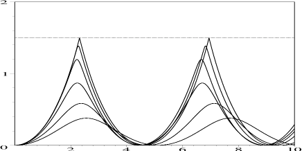
Figure 1: Profiles of the dimensionless surface deformation $\eta$ solution of (4.2) with (4.4) for $c=1$ and $\alpha$ taking the values $0.2$, $0.3$, $0.4$, $0.446$, $0.4499$ and $0.45$, from bottom to top.

The value of the maximum amplitude $\eta_{s}$ reached at wave peaking can be infered from the equation (4.3), it is the value for which the coefficient of the second derivative vanishes, namely

$$\eta_{s}=3\ (c-\frac{1}{2}).$$ (4.5)

We have found actually that this occurs for the initial data (4.4) with the threshold $\alpha_{s}$ given by

$$\alpha_{s}=\frac{3}{10}\ (\frac{5}{2}-c).$$ (4.6)

At the above threshold values, the crest angle can be evaluated as follows.

4.2 Crest angle.

First the integration constant $A$ of (4.3) is evaluated at $\xi=0$ by means of (4.4) and (4.6), we obtain

$$A=\frac{3}{10}(c-\frac{1}{2})(\frac{5}{2}-c).$$ (4.7)

Next we evaluate equation (4.2) at the limit $\xi\to\xi_{s}^{\pm}$ (limit to the left $\xi_{s}^{-}$ or to the right $\xi_{s}^{+}$), where $\xi_{s}$ is the value for which the threshold is reached, namely $\eta(\xi_{s})=\eta_{s}$. We obtain this way the limit of the second derivative by

$$\lim_{\xi\to\xi_{s}^{\pm}}(\eta_{\xi\xi})=\frac{6}{5}v.$$ (4.8)

Figure 2: Values of the crest angle, in degrees, at wave peaking for velocities $c$ in the range $[0.6,\ 1.2]$.

To get the limits of the first derivative we evaluate now equation (4.3) at $\xi=\xi_{s}^{\pm}$. With help of the above value of $A$ we obtain

$$\lim_{\xi\to\xi_{s}^{\pm}}(\eta_{\xi}^{2})=\frac{9}{4}\;(c-\frac{1}{2})\;(\frac{6}{5}c+1),$$ (4.9)

and thus the limit of $\eta_{\xi}$ in $\xi_{s}^{\pm}$ can be either positive or negative. It is then clear that a bounded periodic solution like the one displayed on figure 1 implies the following solution (remember $c>1/2$)

$$\lim_{\xi\to\xi_{s}^{-}}(\eta_{\xi})=-\lim_{\xi\to\xi_{s}^{+}}(\eta_{\xi})=\left[\frac{9}{4}\;(c-\frac{1}{2})\;(\frac{6}{5}c+1)\right]^{1/2}.$$ (4.10)

Last, from the above value of the slope at $\xi_{s}$, the crest angle at wave peaking reads

$$\theta=2\ \arctan\left\{\left[\frac{9}{4}\;(c-\frac{1}{2})\;(\frac{6}{5}c+1)\right]^{-1/2}\right\},$$ (4.11)

and the graph of this expression is plotted on the figure 2. At $c=1$ the angle is $\theta=65\ d^{o}$.

It is worth remarking that the analytic expression of the crest limit angle, which we have cheked on numerical simulations, actually reults in a part from the phenomenological expression (4.6) obtained by observations of numerical simulations of equation (4.2) with boundary data (4.4).

4.3 Peakon solution.

The coefficients of the ODE (4.2) show that periodic solutions hold if $c>1/2$ and a threshold is reached at $c=5/2$ for which waves of vanishing amplitudes are already singular. At this value, the model supports the peakon solution

$$\eta(\xi)=6\exp[-|\xi|/\sqrt{2}],\quad\xi=x-\frac{5}{2}t\ .$$ (4.12)

Remarkably enough, this peakon also appears as the limit of the solitary wave solution when its velocity reaches the value $5/2$.

4.4 Soliton-like waves.

Numerical simulations has revealed the existence of stable soliton-like excitations that travel without deformation at constant speed in the range $[3/2,\ 5/2]$. These are performed by observing that

$$\eta^{(s)}=\frac{\eta_{0}}{\cosh^{2}(\kappa(x-vt-x_{0}))},\quad\eta_{0}=3\ (v-\frac{3}{2}),\quad\kappa=\frac{1}{2}\sqrt{\frac{2v-3}{2v-1}},$$ (4.13)

is an approximate solitary wave solution for (1.4) according to

$$\eta_{t}^{(s)}-\eta_{xxt}^{(s)}-\frac{1}{2}\eta_{xxx}^{(s)}+\frac{3}{2}\eta_{x}^{(s)}+\eta^{(s)}\eta_{x}^{(s)}-\frac{5}{3}\eta_{x}^{(s)}\eta_{xx}^{(s)}-\frac{1}{3}\eta^{(s)}\eta_{xxx}^{(s)}={\cal O}(\kappa^{3}\eta_{0}^{2}).$$ (4.14)

Hence defining

$$v=\frac{3}{2}+\delta\ \Rightarrow\ \{\eta_{0}=3\delta,\ 4\kappa^{2}=\frac{\delta}{1+\delta}\},$$ (4.15)

expression (4.13) tends to the exact solution for $\delta\to 0$ (for which the amplitude $\eta_{0}$ vanishes).

We have performed a series of numerical simulations of (1.4) by first writing it in the frame moving at velocity $v$, namely

$$\eta_{t}+(\frac{3}{2}-v)\eta_{x}-\eta_{xxt}+(v-\frac{1}{2})\eta_{xxx}+\eta\eta_{x}=\frac{5}{3}\eta_{x}\eta_{xx}+\frac{1}{3}\eta\eta_{xxx}.$$ (4.16)

and then by using the following initial-boundary value problem on $x\in[0,L]$

$$\eta(0,t)=\eta_{s}(x,0),\quad\eta(0,t)=0,\quad\eta(L,t)=0,\quad\eta_{x}(L,t)=0,$$ (4.17)

with an initial position $x_{0}=2L/3$ and a velocity

$$v=\frac{3}{2}+\delta,\quad\delta\in]0,1[.$$ (4.18)

The method uses a standard second order implicit finite difference scheme with a mesh grid dimension $0.1$.

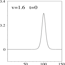
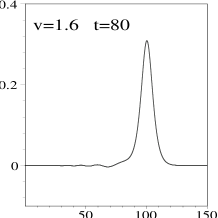
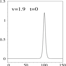
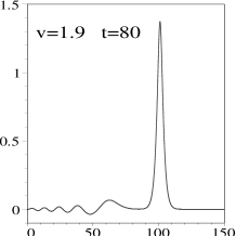
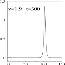
Figure 3: Solitary wave profiles in two examples with $\delta=0.1$ (up) and $\delta=0.4$ (down) in the rest frame of the approximate solution (4.13).

A few typical examples are displayed in fig.3 where we compare the solitary wave to the initial condition. As expected, when $\delta<<1$ (i.e. $v\sim 1.5$) the solitary wave resembles much the initial condition while for larger $\delta$, a pulse reshaping occurs by means of emission of waves (at phase velocity 1). After reshaping, the solution is remarkably stable. When $\delta\to 1$ (i.e. $v\to 5/2$), the solitary wave tends to the peakon solution (4.12).

The found solitary wave solutions behave like solitons do in an integrable system. Indeed, after reshaping, a two-soliton interaction effects only the position of the pulses and does not alter the individual shapes. An example is diplayed in figure 4

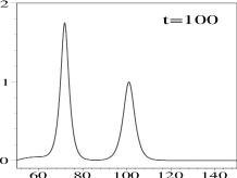
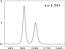
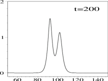
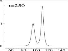
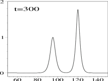
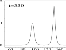
Figure 4: Solitary wave interaction in the rest frame of the soliton at velocity $1.8$, the other soliton having velocity $2$.

Conclusion and comments

The asumed exponential vertical velocity profile has led to a simple model for surface waves on deep water. The derivation is rigorously made by perturbative analysis assuming waves with small aspect ratio parameter, which constitutes a novel approach of the problem.

The resulting model (3.20) sustains periodic waves which tend to peak as their amplitude increase and reach a threshold amplitude $\eta_{s}$ given by (4.5). At this value, the crest angle can be explicitely computed in terms of the velocity by (4.11). However, in the region of the peak, higher order derivatives diverge and the perturbative expansion does not hold anymore. Hence the precise value of the crest angle should be considered with care and the peaking only gives an indication of a behavior due to nonlinearity.

As mentionned in the introduction, it is necessary to release the potential flow approach which is not consistent with the anzatz (2.13). Indeed, assuming the existence of a potential flow $\phi$ by

$$(U,W)=\nabla\phi,$$ (4.19)

the expressions (2.13) and (2.14), together with (2.7), readily provide

$$\phi(x,z,t)=\varphi(x,t)e^{z},\quad\varphi_{xx}+\varphi=0.$$ (4.20)

Although one may obtain nontrivial time-dependence from the Euler system in this particular context, the above linear $x$-dependence of $\varphi(x,t)$ cannot catch nonlinear deformations in a consistent way.

Last but not least, it is remarkable that equation (3.3) possess $k$-dependent coefficients, where $k$ is the wave number of the selected particular wave. It is something new for a model describing a wave profile. Indeed asymptotic non-linear and dispersive long scales models for surface water waves (as Korteweg-deVries, modified KdV, Benjamin-Bona-Mahoney-Peregrine, Camassa-Holm) have $k$-independent coefficients. Conversely, $k$-dependent coefficients are common in the context of modulation of wave trains, as in nonlinear Schrödinger, modified NLS, Davey-Stewartson, etc…

References

- [1] G. B. Whitham, Linear and Nonlinear Waves, (Wiley Interscience, New York, 1974).
- [2] J. Boussinesq, Compte Rendus Acad. Sci. Paris 72, 755-759 (1871).
- [3] D. J. Korteweg and G. deVries, Phil. Mag. (5), 39, 422-443 (1895).
- [4] D.J. Benney, A.C. Newell, J Math Phys 46 (1967) 133
- [5] V.E. Zakharov, J Appl Mech Tech Phys 9 (1968) 190
- [6] C.C. Mei, The Applied Dynamics of the Ocean Surface Waves. Advanced Series on Ocean Engineering, Vol 1, World Scientific, Singapore, 1981.
- [7] F. Dias and C. Kharif, Annu. Rev. Fluid Mech. 31, 310-346 (1999).
- [8] Y. Matsuno, Phys. Rev. Lett. 69,4, 609-611 (1992).
- [9] R. L Seliger and G. B. Whitham, Proc. Roy. Soc. A 305, 1-25 (1968).
- [10] J.-M Vander-Broeck and Y. Agnon, Stud. in Appl. Math. 98, 1-18 (1997).
- [11] A. E. Green, F.R.S., N. Laws and P. M. Nagdhi, Proc. R. Soc. A 338, 43-55 (1974)
- [12] A. E. Green, and P. M. Nagdhi, J. Fluid. Mech. 78, 237-246 (1976), Proc. R. Soc. A 347, 447-473 (1976).
- [13] R. S. Johnson, J. Fluid Mech. 455, 63-82 (2002).
- [14] T. Taniuti and C. C. Weil, J. Phys. Soc. Japan 24, 941 (1968).
- [15] Y. Kodama and T. Taniuti, J. Phys. Soc. Japan 45, 298 (1978).
- [16] A. Jeffrey and T. Kawahara, in Asymptotic Methods in Nonlinear Wave Theory (Pitman Publishing, London, 1982).
- [17] R.A. Kraenkel, M.A. Manna, J.G. Pereira, J Math Phys 36 (1995) 307
- [18] J. Lighthill, Waves in Fluids, Cambridge Univ Press (Cambridge 1978)
- [19] M. A. Manna, J. Phys. A: Math. Gen. 34, 4475-4491 (2001).
- [20] R. Camassa and D. D. Holm Phys. Rev. Lett. 71, 1661-1664 (1993).
- [21] A. Degasperis, M. Procesi, Asymptotic integrability in “Symmetry and Perturbation Theory”, edts A. Degasperis and G. Gaeta, World Scientific (Singapore 1999)
- [22] A. Degasperis, D.D. Holm, A.N.W. Hone, Theor Math Phys 133 (2002) 1463
- [23] H.R. Dullin, G.A. Gottwald, D.D. Holm, Physica D 190 (2004) 1-14