Power and power-logarithmic expansions for travelling-wave solutions of the Burgers-Huxley equation.

Abstract

The Burgers-Huxley equation is studied. All power and power-logarithmic expansions for travelling-wave solutions of this equation are presented. Using the power expansions, some exact solutions of this equation are found.

1 Introduction.

The Burgers-Huxley equation takes the form

$$u_{t}+\alpha uu_{x}=Du_{xx}+\beta u+\gamma u^{2}-\delta u^{3},\qquad D>0,\,\delta>0$$ (1.1)

It is used for description of non-linear wave processes in physics, ecology and economics [2, 1, 3, 5, 4]. The condition of positiveness for coefficients $D$ and $\delta$ follows from the physical meanings of the problems.

The Burgers-Huxley equation is not the exactly solvable one. However some exact solutions can be obtained [6, 7, 8], if we use the singular manifold method [9, 11, 12, 13, 10].

Using travelling waves $u(x,t)=w(z),\ z=x-C_{0}t$ in equation (1.1), we have

$$Dw_{zz}-\alpha ww_{z}+C_{0}w_{z}+\beta w+\gamma w^{2}-\delta w^{3}=0$$ (1.2)

Taking $z=z^{\prime}\sqrt{2D/\delta}$ into consideration, we obtain

$$w_{zz}-\alpha ww_{z}+C_{0}w_{z}+\beta w+\gamma w^{2}-2w^{3}=0$$ (1.3)

where coefficients $\alpha$, $\beta$, $\gamma$ and $C_{0}$ are constants. Primes in (1.3) are omitted.

In the general case equation (1.3) does not pass the Painlevé test, so it is important to find all the asymptotic forms and power expansions for the solutions of this equation. For that we use the power geometry methods [14, 15, 16, 17].

The outline of this paper is as follows. In section 2 we consider the general properties of equation (1.3). In section 3 the power expansions, corresponding to the apexes of the carrier of equation (1.3), are found. Sections 4-9 are devoted to the power and power-logarithmic expansions, corresponding to the edges of the carrier of equation (1.3). In section 10 the examples of exact solutions are given.

2 The carrier of equation (1.3).

The carrier of equation (1.3) consists of points $Q_{1}=(-2,1)$, $Q_{2}=(0,3)$, $Q_{3}=(0,1)$, $Q_{4}=(-1,2)$, $Q_{5}=(0,2)$, $Q_{6}=(-1,1)$. However some of these points can be absent, if coefficients of equation (1.3), corresponding to them, are equal to zero.

If $\beta\neq 0$, the convex hull of the carrier of equation (1.3) is the triangle with apexes $Q_{1}$, $Q_{2}$, $Q_{3}$, presented at fig. 1a. The normal cones for apexes and edges of the carrier of equation (1.3) are given on fig. 1b.

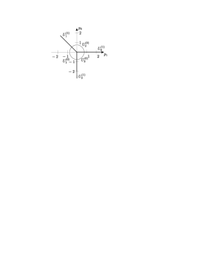
Figure 1: The carrier (a) and the normal cones (b) of equation (1.3) at $\beta\neq 0$

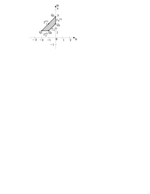
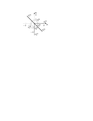
Figure 2: The carrier (a) and the normal cones (b) of equation (1.3) at $\beta=0$, $C_{0}\neq 0$, $\gamma\neq 0$

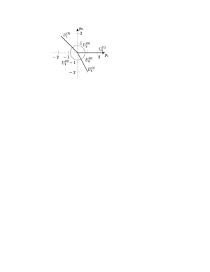
Figure 3: The carrier (a) and the normal cones (b) of equation (1.3) at $\beta=C_{0}=0$ and $\gamma\neq 0$

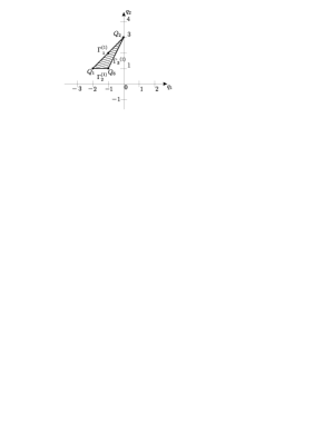
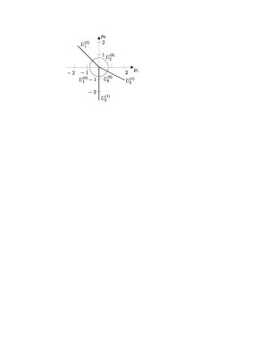
Figure 4: The carrier (a) and the normal cones (b) of equation (1.3) at $\beta=\gamma=0$ and $C_{0}\neq 0$

In the case $\beta=0$, $\gamma\neq 0$ and $C_{0}\neq 0$, the carrier of equation (1.3) is the trapezium, presented at fig. 2a.

If $\beta=0$ and one of the coefficients $\gamma$ or $C_{0}$ is equal to zero, then the carrier and the normal cones of equation (1.3) are given on fig. 3 and fig. 4.

3 Expansions, corresponding to the apexes of the carrier of equation (1.3).

The truncated equation, corresponding to apex $Q_{1}$ of the carrier of equation (1.3), takes the form

$$w_{zz}=0$$ (3.1)

The characteristic polynomial for this equation is

$$\chi(r)=r(1-r)$$ (3.2)

It has roots $r=0$ and $r=1$. Using the condition $\omega(1,r)\in U_{1}^{(0)}$, we have

$$r=0\Rightarrow\omega=-1,z\rightarrow 0$$

$$r=1\Rightarrow\omega=-1,z\rightarrow 0$$

For truncated equation (3.1) we obtain

$$\mathcal{L}(z)=\dfrac{d^{2}}{dz^{2}}\quad\Rightarrow\nu(k)=k(k-1)$$

The proper numbers of the truncated equation (3.1) are $k=0$ and $k=1$. The cone of the problem is $\mathcal{K}=(k:k>r)$. So we have no critical numbers for $r=1$ and one critical number for $k=1$.

The expansion of solutions, corresponding to the truncated solution at $r=0$, takes the form

$$w(z)=c_{0}+c_{1}z+\sum_{s=2}^{\infty}\,c_{s}\,z^{s}$$ (3.3)

where $c_{0}$, $c_{1}$ are the arbitrary constants, other coefficients can be sequentially calculated. Taking into account three terms we obtain

$$w(z)=c_{{0}}+c_{{1}}z+\frac{1}{2}\left(\alpha\,c_{{0}}c_{{1}}-\beta\,c_{{0}}-\gamma\,{c_{{0}}}^{2}-C_{0}c_{{1}}+2{c_{{0}}}^{3}\right){z}^{2}+\ldots$$ (3.4)

The expansion of solutions at $r=1$ is the special case of expansion (3.3) at $r=0$ with $c_{0}=0$. Taking into account three terms we have the expansion for this case

$$w(z)=c_{{1}}z-\frac{1}{2}\,C_{0}c_{{1}}{z}^{2}+\frac{1}{6}\,c_{{1}}\left(-\beta+c_{{1}}\alpha+{C_{0}}^{2}\right){z}^{3}+\ldots$$ (3.5)

Depending on the parameters of equation (1.3), its carrier has two or three more apexes.

Consider the truncated equation, corresponding to apex $Q_{6}=(-1,0)$. This apex exists if $\beta=0$ and $C_{0}\neq 0$ (fig. 2, 4)

$$w_{z}=0$$ (3.6)

Here $r=0$. Condition $\omega(1,r)\in U_{6}^{(0)}$ does not hold, so this apex does not give new expansions.

The other truncated equations, corresponding to the apexes of the carrier of equation (1.3), are the algebraic one and, therefore, also have only trivial solutions.

4 Expansions, corresponding to edge ${\Gamma_{1}}^{(1)}$.

The truncated equation, corresponding to edge ${\Gamma_{1}}^{(1)}$, takes the form

$$w_{zz}-\alpha ww_{z}-2w^{3}=0$$ (4.1)

The outer normal for this edge $N_{1}=(-1,1)$, so we have the normal cone

$$U_{1}^{(1)}=\{\lambda(-1,1),\lambda>0\}$$

Using the condition $\omega(1,r)\in U_{1}^{(1)}$, we obtain $r=-1$, $\omega=-1\Rightarrow z\rightarrow 0$

The solution of truncated equation (4.1) can be described by formula

$$w=\frac{c_{-1}}{z}$$ (4.2)

where

$$2{c_{-1}}^{2}-\alpha c_{-1}-2=0$$ (4.3)

Equation (4.3) has two solutions

$$c_{-1}^{\pm}=\frac{\alpha}{4}\pm\sqrt{\left(\frac{\alpha}{4}\right)^{2}+1}$$

These roots correspond to two asymptotic forms. So it can be two power expansions.

For truncated equation (4.1) we have

$$\mathcal{L}(z)=\dfrac{d^{2}}{dz^{2}}-\alpha\frac{c_{-1}}{z}\dfrac{d}{dz}+\frac{\alpha c_{-1}}{z^{2}}-6\frac{{c_{-1}}^{2}}{z^{2}}$$

Therefore the characteristic equation takes the form

$$\nu(k)=k(k-1)-\alpha c_{-1}k+\alpha c_{-1}-6{c_{-1}}^{2}$$

Using (4.3), we obtain the equation for proper numbers

$$k^{2}-k(1+\alpha c_{-1})-2\alpha c_{-1}-6=0$$

This equation has roots $k_{0}=-2$ and

$$k_{1}=3+\alpha c_{-1}$$ (4.4)

The cone of the problem is $\mathcal{K}=(k:k>-1)$, hence $k_{0}=-2$ is not the critical number.

Let us find, if power expansions exist under the different meanings of the proper number $k_{1}$.

If $\alpha^{2}\neq\dfrac{2a^{2}}{2+a}$, where $a\in Z,\ a>-2$, then there are two power expansions in the form

$$w(z)=\frac{c_{-1}}{z}+\sum_{i=0}^{\infty}{c_{i}z^{i}}$$ (4.5)

where coefficient $c_{-1}$ is either root of equation (4.3), other coefficients are sequentially computed. In particular, $c_{0}$ and $c_{1}$ are determined by formulas

$$c_{0}=\frac{c_{-1}\gamma\alpha+2\gamma-2C_{0}c_{-1}}{4(c_{-1}\alpha+3)}$$

$$c_{1}=\frac{c_{-1}(2\gamma c_{0}-6\,{c_{0}}^{2}+\beta)}{3(c_{{-1}}\alpha+2)}$$

If $\alpha=0$ or $\alpha^{2}=2$, then $k_{1}$ is the critical number for both expansions, and we should control the compatibility conditions: at $\alpha=0$ to $c_{3}$ for both expansions; at $\alpha^{2}=2$ to $c_{5}$ for one expansion and to $c_{1}$ for the other one.

If $\alpha^{2}=\dfrac{2a^{2}}{2+a}$ $(a=1,3,4,5,6,\ldots)$, then $k_{1}$ is the critical number for only one of expansions, and we should examine the compatibility condition to $c_{3+a}$. For the other expansion all coefficients exist and can be uniquely determined.

If the compatibility condition holds, then there is power expansion with one arbitrary constant. This expansion has form, similar to expansion (4.5).

If the compatibility condition fails, then expansion is the power-logarithmic one and takes the form

$$w(z)=\frac{c_{-1}}{z}+\sum_{i=0}^{\infty}{c_{i}(\ln z)z^{i}}$$ (4.6)

where coefficient $c_{-1}$ is either root of equation (4.3) and $c_{i}(\ln z)$ are the polinomials of $\ln z$ and can be uniquely determined.

For example let us consider $\alpha=0$ and $c_{-1}=1$ in details. In this case we obtain the compatibility condition

$$C_{0}(\gamma+2C_{0})(\gamma^{2}+\gamma C_{0}+9\beta-2{C_{0}}^{2})=0$$ (4.7)

If this condition holds, we have power expansion in the form

$$w(z)=\frac{1}{z}+\frac{\gamma-C_{0}}{6}+\frac{z}{36}(6\beta-{C_{0}}^{2}+\gamma^{2})+$$

$$+z^{2}/216(2C_{0}+\gamma)(\gamma^{2}+C_{0}\gamma+9\beta-2{C_{0}}^{2}))+c_{3}z^{3}+\sum_{i=4}^{\infty}c_{i}z^{i}$$

where $c_{3}$ is the arbitrary constant and $c_{i},\,\,i=4,5,6...$ are the constants, that can be sequentially defined.

If the compatibility condition fails (4.7), we obtain the power-logarithmic expansion

$$w(z)= \frac{1}{z}+\frac{\gamma-C_{0}}{6}+\frac{z}{36}(6\beta-{C_{0}}^{2}+\gamma^{2})+$$

$$+\frac{z^{2}}{216}(2C_{0}+\gamma)(\gamma^{2}+C_{0}\gamma+9\beta-2{C_{0}}^{2}))+$$

$$+\left(c_{3}+C_{0}(2C_{0}+\gamma)(2{C_{0}}^{2}-C_{0}\gamma-\gamma^{2}-9\beta)\frac{\ln z}{270}\right)z^{3}+\sum_{i=4}^{\infty}c_{i}(\ln z)z^{i}$$

where $c_{3}$ is the arbitrary constant and $c_{i}(\ln z)$ are the polynomials of $\ln z$, that can be uniquely determined.

5 Expansions, corresponding to edge ${\Gamma_{2}}^{(1)}$.

Edge ${\Gamma_{2}}^{(1)}$ exists, if $\beta\neq 0$ or $C_{0}\neq 0$.

The truncated equation, corresponding to edge ${\Gamma_{2}}^{(1)}$, takes the form

$$w_{zz}+C_{0}w_{z}+\beta w=0$$ (5.1)

The outer normal $N_{2}=(0,-1)$, the normal cone

$$U_{2}^{(1)}=\{\lambda(0,-1),\lambda>0\}$$

The condition $\omega(1,r)\in U_{2}^{(1)}$ does not hold, so there are no power asymptotic forms, corresponding to this edge.

6 Expansions, corresponding to edge ${\Gamma_{3}}^{(1)}$.

This edge exists, if $\beta=\gamma=0$ and $C_{0}\neq 0$.

The truncated equation, corresponding to edge ${\Gamma_{3}}^{(1)}$, takes the form

$$fw_{z}-2w^{3}=0$$ (6.1)

The outer normal for this edge is $N_{3}=(1,-1/2)$, therefore we obtain the normal cone

$$U_{3}^{(1)}=\{\lambda(2,-1),\lambda>0\}$$

Using the condition $\omega(1,r)\in U_{3}^{(1)}$, we have $\omega=1$, $r=-1/2\Rightarrow z\rightarrow\infty$

So the solutions of truncated equation (6.1) can be written as

$$w=\frac{c_{0}}{z^{1/2}},\qquad\text{ }\,\,c_{0}=\pm\sqrt{-C_{0}/4}$$ (6.2)

The characteristic equation here is

$$\nu(k)=C_{0}(k+3/2)$$

We obtain one critical number $k=-3/2$. The compatibility condition does not hold, so we obtain two power-logarithmic expansions

$$w(z)= {\frac{c_{{0}}}{\sqrt{z}}}+{\frac{\alpha}{4z}}+\left(c_{{2}}-{\frac{3c_{{0}}\ln z}{{4C_{0}}}}\right){z}^{-3/2}+$$ (6.3)

$$+\left({\frac{\alpha\,\left({\alpha}^{2}-32\,c_{{0}}c_{{2}}-2\right)}{16{C_{0}}}}-{\frac{3\alpha\ln z}{8C_{0}}}\right){z}^{-2}+\ldots$$

where $c_{0}=\pm\sqrt{-C_{0}/4}$, $c_{2}$ is the arbitrary constant.

7 Expansions, corresponding to edge ${\Gamma_{4}}^{(1)}$.

Edge ${\Gamma_{4}}^{(1)}$ exists, if $\beta=0$, $\gamma\neq 0$ and $C_{0}\neq 0$.

The truncated equation, corresponding to edge ${\Gamma_{4}}^{(1)}$, takes the form

$$C_{0}w_{z}+\gamma w^{2}=0$$ (7.1)

The outer normal for this edge $N_{4}=(1,-1)$, hence we have the normal cone

$$U_{4}^{(1)}=\{\lambda(1,-1),\lambda>0\}$$

Using the condition $\omega(1,r)\in U_{4}^{(1)}$, we obtain $\omega=1$, $r=-1\Rightarrow z\rightarrow\infty$

So the solution of truncated equation can be written as

$$u=\frac{C_{0}}{\gamma}z^{-1}$$ (7.2)

For truncated equation (7.1) we have

$$\mathcal{L}(z)=C_{0}\dfrac{d}{dz}+2\frac{C_{0}}{z^{-1}}\quad\Rightarrow\nu(k)=C_{0}(k+2)$$

As the cone of the problem here is $\mathcal{K}=(k:k<-1)$, we have one critical number $k=-2$.

The compatibility condition is

$$2{C_{0}}^{2}-C_{0}\alpha\gamma-2\gamma^{2}=0$$ (7.3)

If it holds, i.e.

$$\alpha=2\frac{{C_{0}}^{2}-\gamma^{2}}{\gamma C_{0}}$$ (7.4)

then, taking into account four terms, we obtain the expansion near $z=\infty$

$$w(z)=\frac{C_{0}}{\gamma}\frac{1}{z}+\frac{c_{1}}{z^{2}}+\frac{\gamma c_{1}^{2}}{C_{0}z^{3}}+\frac{\gamma^{2}c_{1}^{3}}{C_{0}^{2}z^{4}}+\ldots$$ (7.5)

where $c_{1}$ is the arbitrary constant.

Denote

$$P=2{C_{0}}^{2}-C_{0}\alpha\gamma-2\gamma^{2}$$ (7.6)

If compatibility condition (7.3) fails, i.e. $P\neq 0$, the expansion is the power-logarithmic one. It takes the form

$$w(z)= {\frac{{C_{0}}}{\gamma\,z}}+\frac{c_{1}}{z^{2}}+\frac{P\ln z}{{\gamma}^{3}z^{2}}+\frac{\gamma\,{c_{1}}^{2}}{{C_{0}}z^{3}}-{\frac{c_{1}\,P}{{\gamma}^{2}C_{0}z^{3}}}-{\frac{P\left(3\,{\gamma}^{2}+2\,{{C_{0}}}^{2}\right)}{{C_{0}}{\gamma}^{5}z^{3}}}+$$ (7.7)

$$+\left(2\,{\frac{c_{1}\,P}{{\gamma}^{2}{C_{0}}}}-{\frac{{P}^{2}}{{C_{0}}{\gamma}^{5}}}\right)\frac{\ln z}{z^{3}}+{\frac{{P}^{2}}{{C_{0}}{\gamma}^{5}}}\frac{\ln^{2}z}{z^{3}}+\ldots$$

where $c_{1}$ is the arbitrary constant.

8 Expansions, corresponding to edge ${\Gamma_{5}}^{(1)}$.

Edge ${\Gamma_{5}}^{(1)}$ exists, if $\beta=C_{0}=0$ and $\gamma\neq 0$.

The truncated equation, corresponding to edge ${\Gamma_{5}}^{(1)}$, takes the form

$$w_{zz}+\gamma w^{2}=0$$ (8.1)

The outer normal $N_{5}=(1,-2)$, so the normal cone is

$$U_{5}^{(1)}=\{\lambda(1,-2),\lambda>0\}$$

Using the condition $\omega(1,r)\in U_{5}^{(1)}$, we obtain $\omega=1$, $r=-2\Rightarrow z\rightarrow\infty$

The solution of truncated equation (8.1) can be written as

$$w=-\frac{6}{\gamma z^{2}}$$ (8.2)

For truncated equation (8.1) we have

$$\mathcal{L}(z)=\dfrac{d^{2}}{dz^{2}}-\frac{12}{z^{2}}\quad\Rightarrow\nu(k)=k(k-1)-12$$

Equation $\nu(k)=0$ has roots $k=-3$ and $k=4$. As the cone of the problem is $\mathcal{K}=(k:k<-2)$, here there is one critical number $k=-3$. The compatibility condition holds, if and only if $\alpha=0$. In this case, taking into account three terms, we obtain the expansion near $z=\infty$

$$w(z)=-\frac{6}{\gamma z^{2}}+\frac{c_{1}}{z^{3}}-\frac{\gamma^{4}{c_{1}}^{2}+432}{8\gamma^{3}z^{4}}+\ldots$$ (8.3)

where $c_{1}$ is the arbitrary constant.

If $\alpha\neq 0$, the expansion is the power-logarithmic one

$$w(z)= -\,{\frac{6}{\gamma\,{z}^{2}}}+{\frac{72\,\alpha\,\ln z+7\,c_{{1}}{\gamma}^{2}}{{7\gamma}^{2}{z}^{3}}}-$$ (8.4)

$$- {\frac{648\,{\alpha}^{2}\ln^{2}z-18\,\alpha\,\left(24\,\alpha-7\,c_{{1}}{\gamma}^{2}\right)\ln z}{{49\gamma}^{3}{z}^{4}}}+$$

$$+{\frac{2160\,{\alpha}^{2}-21168+336\,\alpha\,{\gamma}^{2}c_{{1}}-49\,{\gamma}^{4}{c_{{1}}}^{2}}{{392\gamma}^{3}{z}^{4}}}+\ldots$$

where $c_{1}$ is the arbitrary constant.

9 Expansions, corresponding to edge ${\Gamma_{6}}^{(1)}$.

Edge ${\Gamma_{6}}^{(1)}$ exists, if $\beta\neq 0$ or $\gamma\neq 0$.

The truncated equation, corresponding to edge ${\Gamma_{6}}^{(1)}$, takes the form

$$-2w^{3}+\gamma w^{2}+\beta w=0$$ (9.1)

The outer normal $N_{6}=(1,0)$, so the normal cone is

$$U_{6}^{(1)}=\{\lambda(1,0),\lambda>0\}$$

Using the condition $\omega(1,r)\in U_{6}^{(1)}$, we obtain $\omega=1$, $r=0\Rightarrow z\rightarrow\infty$

The solution of truncated equation (9.1) takes the form

$$w=c_{0},\qquad c_{0}=\frac{\gamma\pm\sqrt{\gamma^{2}+8\beta}}{4}$$ (9.2)

Note, that solutions of truncated equation (9.1) are also the solutions of equation (1.3).

If solutions (9.2) are the simple roots, i.e. $\gamma^{2}+8\beta\neq 0$, then there are no additional expansions.

If $\beta=-\gamma^{2}/8\neq 0$, then $c_{0}=\gamma/4$ is the root of the second order. Then, making substitution $w(z)=\gamma/4+v(z)$, for $v(z)$ we obtain equation (1.3) with coefficients $\widetilde{\beta}=0$, $\widetilde{\gamma}=-\gamma/2$ and $\widetilde{C_{0}}=C_{0}-\alpha\gamma/4$. Coefficient $\alpha$ does not change. Let us find expansions of function $v(z)$, which is the solution of equation (1.3) with modified coefficients, near $z=\infty$. Such expansions correspond either edge ${\Gamma_{4}}^{(1)}$ or edge ${\Gamma_{5}}^{(1)}$. Returning to initial notation, we have the expansions for $w(z)$.

If $\alpha=\dfrac{4{C_{0}}^{2}-\gamma^{2}}{\gamma C_{0}}$, $C_{0}\neq 0$, $\gamma\neq 0$ or $\alpha=C_{0}=0$, we obtain the additional power expansion near $z=\infty$. Otherwise, the additional expansion is the power-logarithmic one.

10 Exact solutions of equation (1.3).

In sections 3- 9 we have obtained all the power asymptotic forms to solutions of equation (1.3). All power and power-logarithmic expansions, corresponding to these asymptotic forms, were also found. They are the convergent ones [14, 15, 16].

Under some parameters the obtained power expansions can be summed, and then we obtain the exact solutions of equation (1.3).

Let us give some examples of solutions, that can be found in such a way.

Series (7.5) can be summed. So at $\beta=0$ and $\alpha$, satisfying expression (7.4), we obtain the exact solution of equation (1.3)

$$w(z)=\frac{{C_{0}}^{2}}{\gamma(C_{0}z-c_{1}\gamma)}$$ (10.1)

The summation of expansion (8.3) (which exists if $\alpha=\beta=C_{0}=0$) results in the solution of equation (1.3) in the form

$$w(z)=-\frac{6/\gamma}{(z-z_{0})(z-z_{0}-6/\gamma)}$$ (10.2)

where $z_{0}$ is the arbitrary constant, which can be expressed via $c_{1}$ as $z_{0}=-(36+c_{1}\gamma^{2})/(12\gamma)$.

Using the technique, described in section 9, we obtain the solution

$$w(z)=\frac{\gamma}{4}-\frac{\gamma^{2}}{2C_{0}(\gamma z+2c_{1}C_{0})}$$ (10.3)

on condition that

$$\beta=-\gamma^{2}/8\neq 0,\qquad\alpha=\frac{4{C_{0}}^{2}-\gamma^{2}}{\gamma C_{0}}$$ (10.4)

and solution

$$w(z)=\frac{\gamma}{4}+\frac{12/\gamma}{(z-z_{0})(z-z_{0}+12/\gamma)}$$ (10.5)

if

$$\beta=-\gamma^{2}/8\neq 0,\qquad\alpha=C_{0}=0$$ (10.6)

Here $c_{1}$ and $z_{0}$ are the arbitrary constants.

11 Conclusion.

The Burgers-Huxley equation is used for description of some nonlinear wave processes in physics, economics and ecology . In this work we have studied the travelling-wave solutions of this equation, using the power geometry methods.

We have found all power asymptotic forms and all corresponding expansions of solutions of this equation at the different meanings of parameters. We obtain power and power-logarithmic expansions:

1) power expansion (3.4) near $z=0$ with two arbitrary constants

2) power expansion (3.5) near $z=0$ with one arbitrary constant

3) two expansions near $z=0$, corresponding to asymptotic form (4.2), that can be power one (4.5) as long as power-logarithmic one (4.6) subject to the parameters of equation (1.3)

4) two power-logarithmic expansions (4.2) near $z=\infty$ (if $\beta=\gamma=0$ and $C_{0}\neq 0$)

5) power expansion (7.5) near $z=\infty$, that can be summed and gives the exact solution (10.1) (if $\beta=0$, $\gamma\neq 0$, $C_{0}\neq 0$ and condition (7.3) holds)

6) power-logarithmic expansion (7.7) near $z=\infty$ (if $\beta=0$, $\gamma\neq 0$, $C_{0}\neq 0$ and condition (7.3) fails)

7) power expansion (8.3) near $z=\infty$ with one arbitrary constant, that can be summed and gives the exact solution (10.2) (if $\beta=C_{0}=\alpha=0$ and $\gamma\neq 0$)

8) power-logarithmic expansion (8.4) near $z=\infty$ (if $\beta=C_{0}=0$ and $\gamma\neq 0$, $\alpha\neq 0$)

9) expansion near $z=\infty$, described in section 9 (if $\gamma^{2}+8\beta=0$), that can be power one as long as power-logarithmic one.

The obtained expansions can be used for testing codes at modelling of the wave processes, which can be described by the Burgers-Huxley equation.

This work was supported by the International Science and Technology Center (project B1213).

References

- [1] Loskutov A.Yu., Mikhailov A.S. Introduction to Synergetics. Moskow, Nauka, 1990. 270 p. (in Russian)
- [2] Osipov V.V. The simplest autowaves. /Sorosovskii Obrasovatel’nyi Zhurnal, 1999, pp. 115–121. (in Russian)
- [3] Broadbridge P., Bradshaw B.H., Fulford G.R., Aldis G.K. Huxley and Fisher equations for gene propagation: An exact solution. /ANZIAM J. 44 (2002), 11-20.
- [4] Svirizhev Yu.M. Nonlinear waves, dissipative structures and catastrophes in ecology. Moskow, Nauka, 1987, 368 p. (in Russian)
- [5] Bazyikin A.D. Nonlinear dynamics of interracting populations. Moscow-Izhevsk: Institut of computer researches, 2003. 368 p. (in Russian)
- [6] Kudryashov N.A. Analitical Theory of Non-linear Differential Equations. Moscow-Izhevsk: Institut of computer researches, 2004. 360 p. (in Russian)
- [7] Efimova O. Yu., Kudryashov N.A. The exact solutions of Burgers-Huxley equation. Pricl. Mat. Mekh., 2004. V. 68, No. 3, pp. 462–469.
- [8] Polyanin A.D., Zaitcev V.F., Zhurov A.I. Methods of solutions to nonlinear equations of mathematical physics and mechanics. Moskow, Physmathlit, 2005. 256 p. (in Russian)
- [9] Weiss J., Tabor M., Camevalle G. The Painleve property for partial differential equations. J. Math. Phys., 1983. V.24, No 3, pp. 522–526.
- [10] Chouldhary S. Roy Painleve analysis and special solutions of two families of reaction-diffusion equations. Phys. Letters A, 1991. V. 159, No 4-5, pp. 311–317.
- [11] Kudryashov N.A. The exact solutions of the generalized Kuramoto-Sivashinsky equation. Phys. Letters A, 1990. V. 147, No 5-6, pp. 522–526.
- [12] Kudryashov N.A. On types of nonlinear nonintegrable equations with exact solutions. Phys. Letters A, 1991. V. 155, No 4-5, pp. 269–275.
- [13] Kudryashov N.A., Zargaryan E.D. solitary waves in active-dissipative dispersive media. J. Phys. A: Math. Gen., 1994. V. 29, pp. 8067–8077.
- [14] Bruno A.D. Power geometry in the algebraic and differential equations. Moscow, Nauka, 1998. 288 p. (in Russian)
- [15] Bruno A.D. Asymptotic forms and expansions for solutions of ordinary differential equation. Russian Mathematical Surveys, 2004. V. 59, No. 3, pp. 31-80. (in Russian)
- [16] Bruno A.D. The asymptotical solution of nonlinear equations by means of power geometry. KIAM Preprint 28, Moscow, 2003. (in Russian)
- [17] Kudryashov N.A., Efimova O.Yu. Power expansions for solution of the fourth-order analog to the first Painlevé equation. Chaos, Solitons&Fractals, 2005. (in press)