Effects of microscopic disorder on the collective dynamics of globally coupled maps

Abstract

This paper studies the effect of independent additive noise on the synchronous dynamics of large populations of globally coupled maps. Our analysis is complementary to the approach taken by Teramae and Kuramoto [39] who pointed out the anomalous scaling properties preceding the loss of coherence. We focus on the macroscopic dynamics that remains deterministic at any noise level and differs from the microscopic one. Using properly defined order parameters, an analytical approach is proposed for describing the collective dynamics in terms of an approximate low-dimensional system. The systematic derivation of the macroscopic equations provides a link between the microscopic features of the population (single-element dynamics and noise distribution) and the properties of the emergent behaviour. The macroscopic bifurcations induced by noise are compared to those originating from parameter mismatches within the population.

1 Introduction

A large number of dynamical phenomena are accurately described by deterministic equations. In many cases, however, the deterministic structure of the dynamics is altered by the presence of degrees of freedom others than those included in the equations. Such degrees of freedom cannot be explicitly formulated in the model because their features and actual influence on the observable time evolution are not known. It is commonly assumed that their effect on the deterministic dynamics can be accounted for by additive or multiplicative stochastic terms.

Besides studies of the effects of noise on a single low-dimensional dynamical system, it is only recently that significant attention has been paid to the investigation of the influence of stochastic perturbations on large ensembles of interacting dynamical elements [1, 22]. Here we report on such investigations on large populations of globally coupled nonlinear maps.

Such an interaction scheme, where each population element only feels the average state of the others, has been widely used to model a range of physical, chemical and biological systems, such as arrays of semiconducting elements (Josephson junctions) [43, 28, 44], electrochemical oscillators [42, 15], or continuous-flow stirred tank reactors containing yeast cells [7, 6]. Globally coupled oscillators or maps also constitute a useful approximation for a wider class of spatially extended systems, provided that the range of the interaction is sufficiently large [2]. This may be the case for instance for swarms of flashing fireflies [45, 46], in networks of neurons [38], cultured heart cells [37], or mixed chemical reactions [27].

The interest in globally-coupled systems primarily arises from the a priori non-trivial relation between the dynamics of one single element and the emergent behavior of the population, typically described by macroscopic variables. Given that these macroscopic quantities are often more easily —and sometimes exclusively— accessible to experimental measurements, the non-trivial relation between the two description levels is a central problem not only in the modeling process, but also in the interpretation of experimental measurements. A number of studies have dealt with the weak-coupling regimes of these noiseless systems. Particular attention has been paid to the emergence of a macroscopic dynamics or “non-trivial collective behavior” [12, 13, 4, 24, 30, 29, 26, 5, 23, 36, 32, 33]. Starting from the uncoupled regime, where the mean field is the average of an infinite number of uncorrelated processes and therefore constant, an increase in the coupling among the population elements causes the macroscopic observables to depart from stationarity and to typically display complex collective dynamics, such as clustering and multistability. In the strong-coupling limit, on the other hand, perfect synchronization of the individual elements is observed, a regime of limited interest since the macroscopic evolution is then a trivial copy of the microscopic one.

This limit is the point of departure for the present study of the macroscopic dynamics of large populations of globally and strongly coupled identical maps subjected to microscopic disorder (additive noise or parameter mismatch). Indeed, starting from perfect synchronization offers the hope that the effects of microscopic disorder can be disentangled from the subtleties of the collective regimes typical of the weak-coupling regime.

Apart from the early work of Nichols and Wiesenfeld [28] who studied how synchronous periodic dynamics is affected by noise when the individual map is close to a bifurcation point, the only prominent study of the effect of noise on the synchronous macroscopic dynamics of globally-coupled maps has been conducted by Teramae and Kuramoto [39]. They showed that the unfolding of a chaotic synchronous behavior by weak noise is generically characterized by “anomalous” multiscaling properties of the cloud of points representing the population in the local phase space, in an approach typical of that developed in a series of important papers by Kuramoto and Nakao on non-locally coupled systems [16, 18, 17]. Here we propose an alternative viewpoint on this indication that microscopic additive noise interacts non-trivially with the dynamics of the population.

Starting from the perfect synchronization regime, we observe that the collective motion remains deterministic and apparently low-dimensional at any noise level (up to finite-size effects), at odds with the case where the added stochastic term is the same for every population element [24, 29, 41]. We present an analytical method for deriving the collective behavior from the single element dynamics and the statistical features of the microscopic disorder [9]. Expanding in series the equation of motion of the “mean-field” (i.e. the average of our one-dimensional maps), we obtain an infinite hierarchy of equations for macroscopic variables or order parameters. Our approach is independent of the specific form of the map and of the noise distribution. In particular, the stochastic term needs not to be chosen neither weak nor Gaussian. This method thus provides an answer to the problem of building macroscopic equations of motion starting from the microscopic structure of the population, as discussed e.g. by Cencini et al. [3], and justifies the use of specific systems as representatives of universality classes of noise-induced phenomena. The proposed approach is complementary to the moment expansion method applied in previous studies [11, 30, 40, 31, 22], where the macroscopic equations are derived from the cumulant expansion of the Fokker-Planck or Perron-Frobenius equation for the Langevin dynamics. Our approach differs from the moment expansion techniques in two aspects: first, we do not start from the dynamics of the probability distribution function, but directly from the individual dynamics; second, we do not impose any self-consistency condition, but closure of the equations relies on the dependence on the coupling strength. On the other hand, the order parameter expansion is analogous in spirit to the method recently proposed by Schimansky-Geier and coworkers [14, 22].

The paper is organized as follows. In the next section, we introduce the phenomenology of noise-induced macroscopic bifurcations of large populations of noisy chaotic maps. By means of numerical simulations, we show how the addition of independent noise to each map modifies the mean-field behavior, and we discuss the microscopic features corresponding to different couplings and noise intensities. This picture agrees with the phenomena of noise-induced macroscopic bifurcations that have been studied in the context of continuous-time dynamical systems [34, 47]. Section 3 is devoted to the derivation of the finite-dimensional maps, or reduced systems, which approximate the mean-field dynamics. The detailed analytical derivation through an expansion in order parameters can be found in the appendices. In Section 4 we compare the main features of the collective dynamics of a population of chaotic maps to those exhibited by the reduced systems. In particular, we investigate the connection between our findings and the anomalous scaling properties put forward by Teramae and Kuramoto. Section 5 compares the effect of noise to that of parameter mismatch (“quenched disorder”), and discusses the differences in deriving the reduced systems in the two cases [8, 10]. Section 6 summarizes the main results of the paper, discusses the perspectives of our method and points to a number of possible applications. Part of our results have been presented in [9].

2 Noise-induced collective regimes: phenomenology

Let us consider a population of globally-coupled maps in the formulation introduced by Kaneko [12]. Each individual variable is ruled by the equation:

$$x_{j}\mapsto(1-K)\,f(x_{j})+K\,\langle\,{f(x)}\,\rangle+\xi_{j}(t)\quad j=1,\dots N,$$ (1)

where $f:\mathbb{R}\rightarrow\mathbb{R}$ defines the single-element dynamics, which we require to be smooth for our analytical approach, and $\langle\dots\rangle$ denotes averaging over the entire population. The stochastic term $\xi_{j}(t)$ is chosen at each time step, independently for each population element, according to a distribution of zero average and with the assigned moments $m_{q}$ (the second of which will be denoted $\sigma^{2}$). The coupling strength $K$ ranges from zero, when the population elements are decoupled, to one, when every element is mapped, in the absence of noise, into the same average value. Note that these equations can be recast into a form where the coupling constant can take any positive value, a formulation that is commonly used in the case of globally coupled continuous-time systems.

Next, we use numerical simulations to show how the evolution of the average state variable, the mean-field $X=\langle\,{x}\,\rangle=\frac{1}{N}\sum_{j=1}^{N}x_{j}$, is affected by a change in the noise intensity, as measured by the variance $\sigma^{2}$ of the noise distribution. Together with the coupling strength $K$, $\sigma^{2}$ will be taken as a control parameter for the analysis of the macroscopic dynamics. As already mentioned, we focus on the strong coupling regime $K\in[K_{\rm c},1]$ where the maps synchronize perfectly in the absence of noise.

As one would expect by continuity, if only a small amount of noise is added, the population configuration will be a small perturbation of the fully synchronous regime: the time series of each individual element remains close to that of the mean-field, even in chaotic regimes. This is illustrated in Fig. 1(a) for a population of $2^{22}$ logistic maps of the form $f(x)=1-a\,x^{2}$ with the nonlinearity parameter $a=1.57$ chosen inside the chaotic region, subjected to uniformly distributed noise of zero mean. (All examples presented in this paper will refer to a population of logistic maps, while the application of our approach to populations with different microscopic features will be addressed elsewhere.) When, instead, the noise is strong, the coherence of the motion within the population is lost. The evolution of any element is now blurred by the stochastic term, thus making it difficult to recognize any underlying deterministic behavior from the detection of just one individual time series. Up to finite-size effects, however, the mean field evolves deterministically. The regimes of macroscopic dynamics induced by noise are neither synchronous, since the dynamics of the individual elements are not locked to each other, nor forcedly coherent, in the sense that the distances between units and the mean-field are not always small.

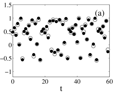
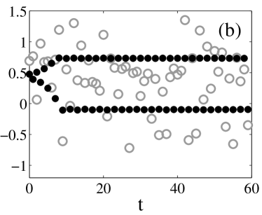
Figure 1: Time series of the mean-field X (black dots) and of one element of the population (open circles) for $K=1$. Population of $N=2^{22}$ logistic maps in the chaotic region ($a=1.57$) with uniformly distributed noise, random initial conditions. (a) In the case of weak noise ($\sigma^{2}=0.05$), the dynamics is a small perturbation of the synchronous, chaotic, noiseless one; (b) In the case of stronger noise intensity ($\sigma^{2}=0.4$), the mean field attains a regular, periodic behavior while the time series of the single population element is scattered by noise.

It is remarkable that, when the noise is sufficiently intense, not only does the mean-field evolution appear to remain low-dimensional, but it can be qualitatively different from the single-element uncoupled dynamics. Figure 1(b) shows for instance that, in the presence of microscopic noise, the mean-field can display regular cyclic behavior in spite of the fact that every element of the population is itself chaotic and noisy. This phenomenon is related to the fact that noise leads the trajectory of any individual element to stay away from the chaotic attractor, so that its dynamics is mainly influenced by the structure (attractive and repulsive manifolds, basins of attraction) of the single-element phase space in the proximity of the asymptotic solution. The coupling among the elements then let these different processes interact so that the probability for one individual system to be mapped into a particular region of its phase space is larger if many other individuals are mapped into similar regions. By averaging over the whole population, the emergent collective dynamics will be mainly determined by how the phase space is structured and, thus, by the global features of the single-element dynamics.

Between the two cases shown in Fig. 1, a series of other macroscopic regimes is observed, ranging from (one or two-band) chaos to cycles of different periods. This can be summarized in the bifurcation diagram of the mean-field shown in Fig. 2(a). (For even higher noise intensities, divergences occur if the single-element map is defined in an interval, as is the case of the logistic map considered here. For unbounded noise distributions, one should in principle consider maps of an unbounded variable.)

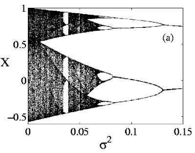
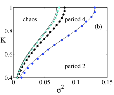
Figure 2: Globally coupled logistic maps ($a=1.57$) with additive uniform noise. (a) Bifurcation diagram of the mean-field as $\sigma^{2}$ is varied at maximal coupling $K=1$. (b) Phase diagram in the $(K,\sigma^{2})$ plane, indicating the first bifurcation lines of the period-doubling cascade (dots: full system, lines: the reduced system to the second degree Eq.(̃8)).

In spite of its resemblance with the bifurcation diagram of a single element, it is important to remember that the macroscopic transitions observed in Fig. 2(a) are directly caused by the presence of noise, while the population parameters are left unchanged. Nonetheless, this macroscopic bifurcation diagram suggests that a low-dimensional map might exist, whose bifurcations reproduce the qualitative changes of the mean-field dynamics. Section 3 IS dedicated to the derivation of such an effective dynamical system. Note further that the observed macroscopic bifurcations are similar to those observed for globally coupled maps with stochastic updating [25], where the uncertainty on the mean field that every element experiences is given by the nature of the updating rather than by an explicit noise term, and for coupled map lattices [20, 21, 19], where the fluctuation of the local field are due to the existence of a finite correlation length.

The microscopic and statistical features of these noise-induced regimes are revealed by looking at three kinds of probability density functions (pdfs): (i) the population (or snapshot) pdf, relative to the values assumed by the individual maps at a specific time, (ii) the individual pdf and (iii) the mean-field pdf, computed over a large time interval for one map of the population and for the mean field, respectively. In the regime of perfect synchronization, the snapshot pdf is a delta peak centered on the value of the mean field, while the two time-averaged pdfs coincide and give the probability measure of the single-element chaotic attractor. When noise is increased, the pdfs are in general modified in a nontrivial manner by the interplay of noise, that tends to blur the individual dynamics and broaden both the population and the individual pdfs, and coupling, that maintains a degree of coherence within the population. As a first example, we consider the case where the coupling is maximal and the mean-field displays a period-two cycle, as in Fig. 1(b). It is easily seen from Eq. (1) that in this limit case the population is distributed exactly like the stochastic term. Accordingly, Fig. 3(b) shows that the population of logistic maps previously considered is at any time step uniformly distributed around the mean field (not shown). This is also reflected in the individual pdf if this is computed at even and odd times separately (Fig. 3(a)). The fact that the individual pdf is slightly broader than the instantaneous pdf and that the mean field pdf is not exactly concentrated on the values taken during the deterministic motion is a consequence of finite size effects. These effects introduce fluctuations that vanish for $N\to\infty$.

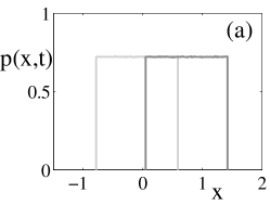
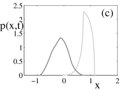
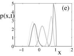
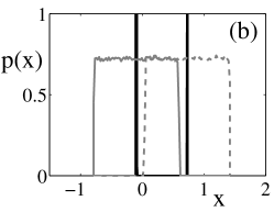
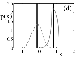
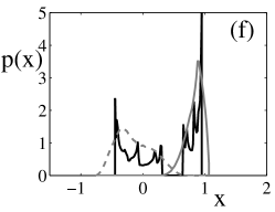
Figure 3: Snapshot pdfs for two (a,c) and five (e) successive time steps and mean field and individual pdfs (b,d,f) for the population of Figure 1: (a-b) Maximal coupling $K=1$ and noise variance $\sigma^{2}=0.016$. (c-d) intermediate coupling $K=0.4$ and noise intensity $\sigma^{2}=0.015$. The mean field displays a period-two cycle, as in (a-b): The interplay between coupling and nonlinearity of the single-element dynamics leads to a nontrivial reshaping of the invidual pdf, that no longer reflects the shape of the noise distribution. (e-f) intermediate coupling $K=0.4$ and noise intensity $\sigma^{2}=0.003$.

Let us now consider the case in which the coupling is not maximal, but still strong enough to ensure perfect synchronization in the absence of noise. For the population considered here, $K=0.4$ is right above the region where two-cluster dynamics occurs. Again, an increase in the noise intensity leads to a seemingly low-dimensional bifurcation diagram. The amount of noise necessary to let the system reach a periodic regime becomes smaller as the coupling strength is decreased. If $K$ is sufficiently weak, a folded structure becomes visible in the first return map of the mean-field, indicating that the macroscopic dynamics is actually embedded in a space of dimension greater than one. The microscopic signature of the system is also significantly changed for intermediate coupling strengths. If we consider $K=0.4$ and $\sigma^{2}=0.015$, where the mean field displays a period-2 cycle, like in the case of maximal coupling discussed above, we notice immediately that the correspondence between the instantaneous pdf and the noise distribution is lost (Fig. 3 (b) and (c)). The individual pdfs for odd/even times still reflect the instantaneous pdf and the mean-field pdf is peaked around the values assumed during the cycle. If the noise intensity is also reduced, so that both the coupling and the noise intensity are sufficiently weak, the possibility of inferring the individual pdf from the instantaneous distribution is lost. For $\sigma^{2}=0.003$, indeed, the mean field displays two-band chaos. Figures 3 (e) and (f) shows that the population distribution changes in time depending on the actual position of the mean field on the macroscopic attractor. The individual pdfs for odd/even times still allow us to recognize a periodicity in the motion, due to the presence of two bands, while the mean field pdf corresponds to the probability measure of the macroscopic attractor.

The phase diagram of our system in the $(K,\sigma^{2})$ parameter plane is summarized in Fig. 2(b). For sufficiently large noise intensity and coupling strength, the macroscopic dynamics is cyclic and of period two. By decreasing the noise intensity or increasing the coupling (for sufficiently low noise) the macroscopic dynamics undergoes a period-doubling bifurcation cascade, leading to regimes of collective chaos. For coupling strength weaker than those displayed in Fig. 2(b), the system shows clustering and multistability. Moving towards the limit of the synchronous (noiseless) regime, the population pdf becomes bimodal or multimodal and its moments take values significantly larger than those of the noise distribution. This transition to clustered solutions, where the population is divided into subgroups placed at finite distance, is related to the anomalous scaling properties reported by Teramae and Kuramoto, see Sec. 4. We note finally that these findings are in agreement with those of Shibata, Chawanya and Kaneko [35] who observed that very weak noise is sufficient to drastically reduce the dimensionality of the macroscopic dynamics at weak coupling.

3 Order parameter expansion

In this section we present our order parameter expansion and its truncation to finite-dimensional systems. The method is formally analogous to that formulated in our recent publications [8, 10] for populations with parameter mismatch, but relies on different closure assumptions based on the different microscopic properties of the noisy system. These differences and their implications will be discussed in Sect. 5. We only present here the main ideas behind our derivation and refer the reader to Appendix A for details.

The iterate of the mean-field can be formally computed by averaging the individual dynamics Eq. (1) and by performing the change of variables: $x_{j}=X+\epsilon_{j}$. In this way, the dynamics of the oscillators around the mean-field is decoupled from the deterministic behaviour of their average. By expanding in series the single-element map $f$ around the mean-field, one obtains:

$$X\mapsto\langle\,{f(x)}\,\rangle=f(X)+\sum_{q=1}^{\infty}\>\frac{1}{q!}\>\mathcal{D}^{q}f(X)\>\langle\,{\epsilon^{q}}\,\rangle+\langle\,{\xi}\,\rangle$$ (2)

where $\mathcal{D}^{p}f$ is the $p$-th derivative of the single-element dynamics, and the last term, reflecting finite-size fluctuations, vanishes in the infinite-size limit for zero-mean noise distributions. Note that $X$ is coupled to other macroscopic variables, namely to the moments of the population instantaneous pdf, defined by:

$$\Omega_{q}:=\langle\,{\epsilon^{q}}\,\rangle\hskip 170.71652ptq\in\mathbb{N}.$$ (3)

From now on we will refer to these macroscopic observables as order parameters. This is not only to avoid confusion with the noise distribution moments, but also to stress that these are the degrees of freedom relevant for a macroscopic description. Moreover, as will be shown in Sec. 5, in the more general case in which the elements are not identical, the same expansion leads to order parameters that do not coincide with the moments of the population pdf.

The iterates of the order parameters can be computed by following the same scheme of variable change and averaging the iterates of the displacements $\epsilon_{j}$, obtained after a Taylor expansion of the individual maps. This yields:

$$\Omega_{q}\mapsto \sum_{i=0}^{q}\binom{q}{i}(1-K)^{i}\left\langle\left(\xi-\langle\,{\xi}\,\rangle\right)^{q-i}\left[\sum_{p=1}^{\infty}\frac{1}{p!}\mathcal{D}^{p}f(X)\left(\epsilon^{p}-\Omega_{p}\right)\right]^{i}\right\rangle\;.$$

Observing that, as a consequence of the fact that the displacements $\epsilon_{j}$ and the noise are uncorrelated variables, $\langle\,{h(X,\epsilon)\>\xi^{q}}\,\rangle=\langle\,{h(X,\epsilon)}\,\rangle\>\langle\,{\left(\xi-\langle\,{\xi}\,\rangle\right)^{q}}\,\rangle$, and taking the limit $N\to\infty$, the equations for the order parameters become:

$$\Omega_{q}\mapsto m_{q}+\sum_{i=1}^{q}\binom{q}{i}(1-K)^{i}\>m_{q-i}\left\langle\left[\sum_{p=1}^{\infty}\frac{1}{p!}\mathcal{D}^{p}f(X)\left(\epsilon^{p}-\Omega_{p}\right)\right]^{i}\right\rangle,$$

where $m_{q}=\langle\,{\left(\xi-\langle\,{\xi}\,\rangle\right)^{q}}\,\rangle$ is the $q$-th moment of the noise distribution.

Such equations compose an infinite-dimensional dynamical system describing the evolution of all order parameters, formally equivalent, in the infinite-size limit, to the original system. The dependence of these equations on powers of $(1-K)$ allows us to truncate them in the region of strong coupling. We call such a truncation to the $n$-th power in $(1-K)$ the reduced system of $n$-th degree. In Appendix A we demonstrate that for any polynomial map of degree $P$ the reduced system at $n$-th degree is a map with $n$ independent variables (the mean field $X$ and the order parameters form the second to the $n$-th) and $(n-1)P$ slaved variables (the order parameters from number $n+1$ to number $n\>P$). The remaining order parameters are constantly equal to the moments of the noise distribution. The reduced system to the $n$-th degree can thus be cast in the form:

$$\begin{cases}X\mapsto&f(X)+\sum_{q=2}^{n}\>A_{q}(X)\Omega_{q}\\ \rule[0.0pt]{0.0pt}{19.91692pt}\Omega_{q}\mapsto&m_{q}+\sum_{i=1}^{q}\binom{q}{i}(1-K)^{i}\,m_{q-i}\,\Gamma_{i}(X,\Omega_{2},\dots\Omega_{n})\hskip 19.91692ptq=2,\dots n\end{cases}$$ (4)

where the functions $A_{q}$ and $\Gamma_{i}$ of the mean-field and of the order parameters relevant to the chosen approximation level contain the first $2P$ moments of the noise distribution as population-level parameters. As illustrated in Appendix A, such expressions can be systematically derived in two steps: first, one writes the order parameters $\Omega_{n+1}\dots\Omega_{nP}$ as linear combinations of $\Omega_{2}\dots\Omega_{n}$, then these are plugged into Eq. (2) and into the first $n$ terms of Eq. (3).

As a first example, consider the reduced system of zeroth degree:

$$X\mapsto f(X)+\sum_{q=1}^{\infty}\>\frac{1}{q!}\>\mathcal{D}^{q}f(X)\>m_{q}.$$ (5)

This scalar map accounts exactly for the macroscopic dynamics when the coupling is maximal (see, e.g. Fig. 2) and provides a first approximation for the dynamics at very strong coupling.

Equation (5) naturally contains the interplay between nonlinearities of the uncoupled map, represented by the derivatives of the single-element dynamics, and the features of the noise distribution, given by its moments. In particular, it allows us to infer that, if the single-element dynamics is polynomial, only a finite number of the noise distribution moments $m_{q}$ will influence the macroscopic dynamics. This induces a relation of equivalence onto the space of the distributions for the stochastic term. These distributions can thus be divided into classes on the bases of their effect on the mean-field.

Being independent of $K$, the reduced system to zeroth degree obviously cannot describe the change in the bifurcation values when the coupling is lowered, and higher degree truncations need to be considered. With zero-average symmetric noise distributions (such as envisaged here), only even-degree order parameters come into play.

The reduced system to the second degree is the first truncation that displays an explicit dependence on the coupling constant $K$. Such a truncation differs from the Gaussian approximation of the population pdf, commonly used for closing cumulant expansions [47], by which the population pdf is approximated as being completely characterized by its first two moments. Our closure assumptions are instead based on the strength of the coupling and take into account also for cases in which neither the noise distribution nor the snapshot pdfs are Gaussian. However, in the truncations at lowest degree, the equations obtained with the two different assumptions may coincide.

In order to compute the two-dimensional reduced system, we exploit the recurrence relation for the order parameters:

$$\Omega_{q+2}=m_{q+2}-\frac{(q+2)(q+1)}{q(q-1)}\frac{m_{q}}{m_{q-2}}(m_{q}-\Omega_{q})$$

that can be derived from Eq. (12). This allows us to express every order parameter as a function of $\Omega_{2}$ through the computation of a telescopic sum, that yields:

$$\Omega_{q}=m_{q}-\frac{q(q-1)}{2}\>m_{q-2}\>\left(\sigma^{2}-\Omega_{2}\right).$$ (6)

One of the consequences of the last equation is that all the odd order parameters are given by the corresponding moments of the noise distribution.
Equation (3) can be rewritten, expliciting the squared term, as:

$$\Omega_{q}\mapsto m_{q}+\frac{q(q-1)}{2}\>(1-K)^{2}\>m_{q-2}\sum_{p,r=1}^{\infty}\frac{1}{p!\>r!}\>\left[\mathcal{D}^{p}\,f(X)\right]\>\left[\mathcal{D}^{r}\,f(X)\right]\>\Omega_{p+r}$$

$$-\frac{q(q-1)}{2}\>(1-K)^{2}\>m_{q-2}\left[\sum_{p=1}^{\infty}\frac{1}{p!}\>\mathcal{D}^{p}\,f(X)\>\Omega_{p}\right]^{2}.$$

Substituting in this last equation the recurrence Eq. (6), one gets the two-dimensional reduced system:

$$\begin{cases}X\mapsto&f(X)+\alpha_{0}(X)+\alpha_{1}(X)\>\Omega_{2}\\ \rule[0.0pt]{0.0pt}{17.07164pt}\Omega_{2}\mapsto&\sigma^{2}+\>(1-K)^{2}\left[\gamma_{0}(X)+\gamma_{1}(X)\>\Omega_{2}+\gamma_{2}(X)\>\Omega_{2}^{2}\>\right].\end{cases}$$ (7)

The nonlinear dependence from the mean field is contained into the coefficients:

$$\alpha_{0}(X)=\sum_{q=2}^{\infty}\>\frac{1}{q!}\>\mathcal{D}^{q}f(X)\left[\>m_{q}-\binom{q}{2}\>m_{q-2}\>\sigma^{2}\right]$$

$$\alpha_{1}(X)=\frac{1}{2}\sum_{q=2}^{\infty}\>\frac{1}{(q-2)!}\>\mathcal{D}^{q}f(X)\>m_{q-2}$$

$$\gamma_{0}(X)=-\left[\alpha_{0}(x)\right]^{2}+\beta_{0}(X)-\beta_{1}(X)\>\sigma^{2}$$

$$\gamma_{1}(X)=\beta_{1}(X)-2\>\alpha_{0}(X)\,\alpha_{1}(X)$$

$$\gamma_{2}(X)=-\left[\alpha_{1}(X)\right]^{2},$$

with:

$$\beta_{0}(X)=\sum_{q,p=1}^{\infty}\frac{m_{q+p}}{q!\>p!}\>\left[\mathcal{D}^{q}\,f(X)\right]\>\left[\mathcal{D}^{p}\,f(X)\right]$$

$$\beta_{1}(X)=\sum_{q,p=1}^{\infty}\frac{m_{q+p-2}}{q!\>p!}\binom{q+p}{2}\left[\mathcal{D}^{q}\,f(X)\right]\>\left[\mathcal{D}^{q}\,f(X)\right].$$

These terms originate according to the nonlinearities of the single-element dynamics and to the moments of the noise distribution. If $f$ is a polynomial of degree $P$, the highest moment of the noise distribution that occurs as a population-level parameter is $m_{2P}$, while the moments of higher orders are unimportant to this approximation level.

The reduced systems obtained by successive approximations of the order parameter expansion provide the link between the microscopic properties of the population and the mean field dynamics. In the following section, we only consider truncations up to the fourth degree for quadratic maps, but an algorithm can easily be implemented for computing the reduced system at $n$-th degree for an arbitrary polynomial map.

The formalism introduced here allows us to conclude that the higher the nonlinearity of the single-element dynamics is, the stronger the noise intensity must be to observe its effect on the macroscopic dynamics. A second important conclusion that can be drawn from the order parameter expansion is that the microscopic map determines which of the noise distribution moments the mean field behaviour is sensitive to. These two facts suggest that even if only averaged observables are accessible, information about the features of the single-element dynamics can be inferred from purely macroscopic measurements.

4 Macroscopic bifurcation diagram and anomalous fluctuations.

In this section we show that the reduced systems are able to capture the main properties of the collective dynamics. In fact, as will be reported elsewhere, the quality of the agreement goes well beyond these main properties, and the reduced systems account, as their degree is increased, for finer and finer features of the collective dynamics.

Figure 2(b) displays the bifurcation lines of the reduced system of second degree for the population of logistic maps considered in the previous section. In this case Eq. (7) is the two-dimensional map:

$$\begin{cases}X\mapsto&1-a\,X^{2}-a\>\Omega_{2}\\ \Omega_{2}\mapsto&\sigma^{2}+(1-K)^{2}\>a^{2}\left[m_{4}-6\,\sigma^{4}+(4X^{2}-\Omega_{2}+6\>\sigma^{2})\>\Omega_{2}\right].\end{cases}$$ (8)

The dependence of the reduced system on the variance and kurtosis of the noise distribution, as well as on the coupling strength, is seen to reflect the qualitative changes in collective behaviour that are observed for the population.

For low coupling intensities, that is approaching the region where the synchronous regime becomes unstable for the noiseless maps, the agreement between the reduced and the full system deteriorates up to the point where the solutions of Eq. (8) diverge. One then needs to consider higher-degree truncations, which indeed, account better for the actual dynamics. For the large-coupling region shown in Fig. 2(b), however, the improvement is hardly visible and the second-degree reduced system provides a satisfactory description of the collective dynamics.

Strikingly, the quality of the second-degree reduced system is such that this simple two-dimensional map also accounts for the onset of the anomalous scaling properties uncovered by Teramae and Kuramoto [39]. In Fig. 4(a) we first show that anomalous scaling is observed for globally coupled noisy logistic maps, in agreement with the claims of universality made by these authors. Note, though, that anomalous scaling is only observed over a finite range of noise strengths: the anomalous behaviour sets in for sufficiently large, although weak, noise, and disappears for noise fluctuations of order one, i.e. of the order of the size of the attractor. We interpret the normal scaling observed at very weak noise as being due to the fact that the individual pdf is maintained below the critical scale that separates microscopic from macroscopic chaos, as defined by Cencini et al. in [3]. Below this scale, noise does not alter the structure of the macroscopic phase space, so that normal scaling is observed. When the cloud of points becomes large enough to cause, for instance, the connection of two neighboring folds of the noiseless system invariant manifolds, the mean-field attractor undergoes a macroscopic bifurcation. We trace the origin of anomalous scaling back to such macroscopic (albeit possibly infinitesimally small) noise-induced changes which are typically accompanied by intermittent behavior. As already mentioned, the reduced system to second degree is sufficient to explain the appearance of anomalous fluctuations in the second moment of the individual pdf, i.e. the order parameter $\Omega_{2}$. In Figs. 4(b,c), we compare the full and the reduced system by plotting the ratio between the second moment of the instantaneous distribution for the population and $\sigma^{2}$, the variance of the noise. The agreement is quantitative, and improves in the region of low coupling when the reduced system to fourth degree is considered (not shown). It is not clear whether our finite-dimensional reductions of the full infinite-dimensional system are able to exhibit anomalous scaling; indeed the region where scaling is observed over many decades is limited to the proximity of the transition to clustering/loss of full synchrony, where our low-degree approximations fail.

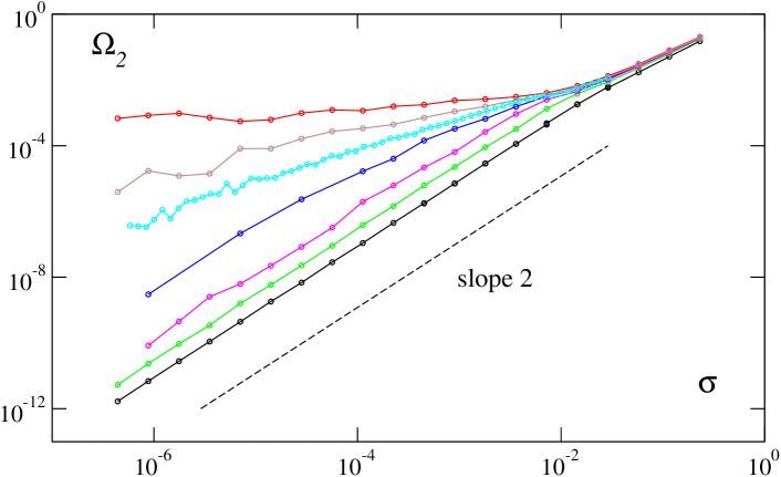
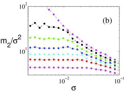
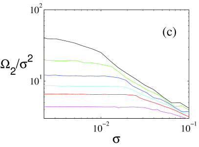
Figure 4: Anomalous scaling in populations of globally-coupled noisy logistic maps. (a) variance of the individual pdf vs noise strength. From top to bottom curve: $K=0.3$, 0.31, 0.315, 0.32, 0.33, 0.35, 0.4 (population of about $2^{18}$ maps). For the smallest coupling, the second moment tends to a constant value, an indication of the existence of clustered solutions. (b) Ratio between the second moment of the snapshot distribution and the noise distribution variance $\sigma^{2}$ (from top to bottom $K=0.32,0.34,0.36,0.38,0.4,0.42,0.46$). These data have been obtained by direct simulation of the Perron-Frobenius operator; (c) same as (b) but from simulations of Eq. (8) (from top to bottom $K=0.34,0.36,0.38,0.4,0.42,0.46$). For too low coupling (e.g. $K=0.32$) the reduced system diverges.

5 Collective dynamics of populations with different kinds of microscopic disorder

Parameter mismatch and noise are often viewed as two fundamental ways of representing microscopic disorder. In the first case, the mismatch within the population is traced back to the existence of a time-independent distribution in the properties of single-elements. In the second case, the difference among individuals is due to some dynamical processes that cannot be described at the chosen observation level and are generically described by noise terms. The persistence of the main features of the population dynamics after the introduction of a small amount of individual diversity and/or noise is usually regarded as a proof of the robustness of a phenomenon and, consequently, of its relevance in the description of real-world systems. Here, we propose to use the order parameter expansion approach to perform a systematic comparison between the effects of these two sources of disorder. The reduced system for noisy maps derived in Sect. 3 is compared to that obtained, under different closure assumptions [8, 10], for populations with parameter mismatch. To this aim, we draw the microscopic disorder according to the same assigned distribution in both cases.

The equations describing populations with parameter mismatch have the same form as those with additive noise Eq. (1):

$$x_{j}\mapsto(1-K)\,f(x_{j})+K\,\langle\,{f(x)}\,\rangle+p_{j}\quad j=1,\dots N,$$ (9)

but the additive term $p_{j}\in\mathbb{R}$ is now assigned once and for all. According to the choice we made for the case of noisy maps, we consider a uniform disorder distribution with mean $p_{0}=0$, variance $\sigma^{2}$ and kurtosis $m_{4}$. The parameters $p_{j}$ will be taken equally spaced on the support of such a distribution in order to let the bifurcation diagram be insensitive to the fluctuations related to a resampling.

To obtain the equations governing the mean field evolution, we apply again an order parameter expansion by averaging Eq. (1) and by performing the change of variables $\epsilon_{j}=x_{j}-X$. Analogously to what was done in the more general case of a dependence of $f$ on the distributed parameter [10], the expansion can be closed under the assumption that the collective dynamics is coherent. The coherency condition $||x_{j}-X||\ll 1$ states that the population dynamics keeps all the individuals within a small neighborhood of the mean field state. This assumption allows us to neglect terms of degree larger than one in $\epsilon_{j}$, independently of the population size.
The reduced system for parameter mismatch has the form:

$$\begin{cases}\rule[-11.38109pt]{0.0pt}{17.07164pt}X\mapsto&\>f(X)+\frac{1}{2}\left[d_{x}f(X)\right]^{2}\,\Omega_{2}\\ \rule[-11.38109pt]{0.0pt}{17.07164pt}W\mapsto&\>\sigma^{2}+(1-K)\,d_{x}f(X)\,W\\ \Omega_{2}\mapsto&\>\sigma^{2}+2\,(1-K)\,d_{x}f(X)\,W+(1-K)^{2}\\ &\times\left\{\left[d_{x}f(X)\right]^{2}\,\Omega_{2}+\frac{1}{4}\left[d_{xx}f(X)\right]^{2}\left(m_{4}-\Omega_{2}^{2}\right)\right\}.\rule{0.0pt}{17.07164pt}\end{cases}$$ (10)

Hence, the mean field is coupled to the second moment of the snapshot distribution $\Omega_{2}=\langle\,{\epsilon_{j}^{2}}\,\rangle$, which is, in turn, influenced by the “shape” order parameter $W=\langle\,{p_{j}\,\epsilon_{j}}\,\rangle$ [10]. As for the reduced system Eq. (8), obtained in the case of noise, the population-level parameters that naturally emerge in the expansion as macroscopically relevant are the coupling strength $K$ and the moments, namely the variance $\sigma^{2}$ and fourth moment $m_{4}$, of the parameter distribution.

In the case of logistic maps $f(x)=1-ax^{2}$ the reduced system to second order Eq. (10) is:

$$\begin{cases}\rule[-11.38109pt]{0.0pt}{17.07164pt}X\mapsto&\>1-a\,X^{2}-2\,a\,\Omega_{2}\\ \rule[-11.38109pt]{0.0pt}{17.07164pt}W\mapsto&\>\sigma^{2}-2\,a\,(1-K)\,X\,W\\ \rule[-5.69054pt]{0.0pt}{17.07164pt}\Omega_{2}\mapsto&\>\sigma^{2}-4\,a\,(1-K)\,X\,W+a^{2}\,(1-K)^{2}\,\left[m_{4}+\left(4\,X^{2}-\Omega_{2}\right)\,\Omega_{2}\,\right]\end{cases}.$$ (11)

For maximal coupling, this description converges to the same scalar equation as obtained for noisy populations. In this limit, the shape parameter and the population variance become uncoupled and coincide. From a microscopic point of view, this corresponds to the fact that the snapshot pdf for $K=1$ in both cases equals the distribution of disorder, that is solidly displaced with the mean field motion (hence, Figs. 3 (a-b) provide a microscopic picture valid for both sources of disorder). The only difference is that in the case of parameter mismatch the oscillators maintain the order of their arrangement, while in the case of noise they randomly exchange their positions at each time step. A straightforward consequence of this is that even if the macroscopic dynamics is indistinguishable for infinite population size, in the case of noise it depends essentially on the number of elements composing the population, while this dependence is much weaker for parameter diversity. In the following, we discuss why this difference exists for every value of the coupling.

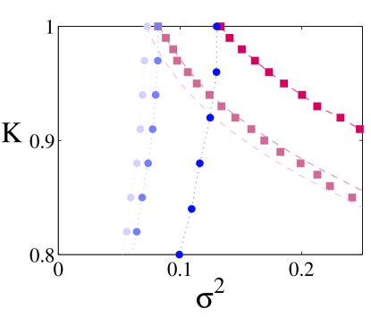
Figure 5: Period-doubling bifurcation lines for the population of noisy maps studied in Sec. 2 (full system, dots and reduced system to the second degree Eq. (8), dotted lines) and for Eq. (9) (population of $N=64$ logistic maps, squares and reduced system Eq. (11), dashed lines). The bifurcation parameters are the variance of the parameter or noise distribution $\sigma^{2}$ and the coupling strength $K$. In the top-right region of the diagram the mean field is stationary for both forms of disorder, while for still larger $\sigma^{2}$ the macroscopic dynamics diverges.

When the coupling is less than maximal, on the other hand, we expect to observe differences in the macroscopic regimes induced by parameter mismatch and noise. These differences can be visualized by plotting in the plane $(\sigma^{2},K)$ the period doubling bifurcation lines for the mean field motion (Fig. 5). While for weaker couplings a low intensity of noise is sufficient to drive the system out of the chaotic region, the opposite happens if the microscopic disorder is due to a diversity in the parameters. Indeed, in this case the region where the mean field displays chaotic behaviour becomes larger for smaller $K$. This property of the macroscopic dynamics is captured by the reduced system Eq. (10), whose bifurcation lines provide a good quantitative approximation of those determined by numerically simulating the population.

As mentioned above, another important difference between the two sources of microscopic disorder is the dependence of the collective dynamics on the population size. This is captured by the difference in the condition of validity of the reduced systems that describe the macroscopic dynamics. As pointed out in Sec. 3, the derivation of Eq. (4) is based on the assumption that the population is infinitely large, while the mean field of finite populations undergoes fluctuations that scale as $1/\sqrt{N}$. On the other hand, Eq. (4) has been derived without making any assumption on the system size, but rather under the hypothesis that the collective regimes are coherent. Hence, in the case of parameter mismatch the system size is expected to play a minor role for the qualitative features of the macroscopic dynamics. The weak dependence on the system size of the mean field behaviour for populations with parameter mismatch is confirmed by the numerical simulations and can be understood by looking at the characteristics of the snapshot distribution. Figure 6 displays the instantaneous pdfs for the populations with parameter mismatch and additive noise in regimes where the mean field has a period-two attractor. If the disorder is due to parameter mismatch, the shape of the instantaneous pdf is little affected by the number of points that identify its profile, along which the oscillators maintain their ordered configuration. If noise is present, on the other hand, reducing the population size alters the shape of the instantaneous pdf at every time step, broadening it with respect to the infinite-size limit distribution, and, hence, affecting the mean field dynamics in an unpredictable way.

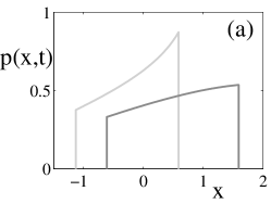
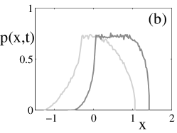
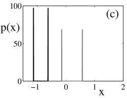
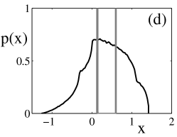
Figure 6: Snapshot pdfs (at even and odd times) (a-b) and mean field and individual pdfs (c-d) for a macroscopic period-two regime in populations of logistic maps with (a-c) parameter mismatch ($\sigma^{2}=0.6$, $K=0.9$) and (b-d) additive noise ($\sigma^{2}=0.4$, $K=0.7$).

Another conclusion that can be drawn by looking at Figs. 6 (a) and (b) is that the snapshot distribution reflects the source of microscopic diversity that underlies collective behaviour. Thus, given a certain mean-field dynamics one should be able, in principle, to identify the character of the microscopic disorder by looking at the statistical properties of the instantaneous distribution. This is even more evident if we compare the individual pdfs, obtained from the time series of an individual map within the populations with different nature of microscopic disorder. Figures 6 (c) and (d) illustrate this in the case when the two populations possess qualitatively similar macroscopic regimes, that is they are both periodic of period two. Correspondingly, the mean field pdf consists in two Dirac delta functions centered on the values assumed by the cycle. Although the two populations cannot be distinguished at a macroscopic level, the difference is evident if one considers the individual pdfs. In the case of parameter mismatch, the probability distribution of an individual time series is identical to the mean field pdf, but centered on shifted values. This is a consequence of the fact that one oscillator in the population maintains its position relative to the population average. When the disorder is due to noise, on the other hand, the individual pdf is broad, since the trajectory of one individual within the population is blurred by the stochastic term. Having access to a macroscopic-level and a microscopic-level observable, such as the time series of the average and of one element within the population, these differences can be used to identify the kind of disorder that is the main determinant of the emergent population dynamics.

6 Discussion

In this paper, we have described the transition from full synchronization to disorder-induced collective dynamics in large populations of globally coupled maps, a prototype for the study of systems with many degrees of freedom. The influence of microscopic variability on the macroscopically accessible degrees of freedom is particularly relevant in modeling biological populations and in the interpretation of experimental results.

Here we have mostly treated the case of additive noise, and focused on its influence on the collective dynamics, a viewpoint complementary to that adopted by Teramae and Kuramoto [39]. We argued that noise induces changes in the macroscopic dynamics which are probably at the origin of the anomalous scaling properties reported by these authors.

We have presented the systematic derivation of finite-dimensional reduced systems which were showed to account quantitatively and with increasing accuracy for the collective dynamics of the full system. The reduced systems link the dynamics of the mean-field to microscopic properties of the population, such as the single-element dynamics parameters and the moments of the noise distribution. Remarkably, the reduced systems were shown to exhibit anomalous scaling themselves. We believe this is because both the full and the reduced system share the folded, fractal phase-space structure at the origin of the macroscopic bifurcations leading to anomalous scaling. This conjecture should be addressed in the future, in an effort to link the scaling properties of the collective dynamics attractors to the anomalous scaling of the population distribution.

Finally, we addressed the effects on the collective dynamics of strongly coupled maps of different sources of microscopic disorder. The results obtained on the noise-induced mean-field bifurcations have been compared to those obtained when the noise is “quenched”, that is when there is a parameter mismatch within the population. Even though in both cases the macroscopic dynamics is qualitatively modified as the disorder is increased, these changes differ in general depending on the origin of the microscopic disorder and we argued that this can be used in the interpretation of experimental data, even when only macroscopic observables are accessible.

The analytical approach presented in this paper allows us to derive in a systematic manner macroscopic equations ruling the effective dynamics of populations of globally and strongly coupled dynamical system. Although here we only presented results relative to maps, we envisage that a similar approach might be applied to continuous-time systems.

Acknowledgments

S. De Monte acknowledges support from the ESF program REACTOR and from the Danish Natural Science Foundation.

Appendix A Order parameter expansion for noisy maps

From Eq. (3), one can see that, if the map is a polynomial of order $P$ and the expansion is truncated to the $n$-th degree in $(1-K)$, then the mean-field is coupled to the order parameters from the second to the $P$-th. The iterates of such $n-1$ variables contain order parameters from the second up to the $nP$-th degree. The dimensionality of the macroscopic map is hence equal to $nP$, while the remaining infinite degrees of freedom, of larger degree, are constantly equal to the moments of the noise distribution.

We now demonstrate that such a $nP$-dimensional truncation can be simplified further and reduced to a system of $n$ equations independently of the degree of nonlinearity of the single-element dynamics. In order to show this, let us define the vector ${\bf\Gamma}$ containing the terms that multiply $(1-K)^{i}$ ($i<nP$) in the following way:

$$\Gamma_{1}= 0$$

$$\Gamma_{i}= \left\langle\left[\sum_{p=1}^{P}\frac{1}{p!}\mathcal{D}^{p}f(X)\left(\epsilon^{p}-\Omega_{p}\right)\right]^{i}\right\rangle\hskip 14.22636pti=2,\dots,n\,P.$$

Let us call ${\bf\Omega}=\left\{\Omega_{1},\dots\Omega_{nP}\right\}$ the vector collecting the first $n\,P$ order parameters and ${\bf m}$ the vector composed by the corresponding moments of the noise distribution. We will show that only the first $n-1$ order parameters are independent variables in the macroscopic dynamics, while the other elements of the vector $\Omega$ can be expressed as linear combinations of appropriate functions of the first ones.

The truncation to $n$-th degree of Eq. (3) can be written as:

$${\bf\Omega}-{\bf m}\mapsto\mathcal{C}\>{\bf\Gamma},$$ (12)

where $\mathcal{C}$ is an $nP\times nP$ matrix whose entries are:

$$\begin{cases}\vspace{1mm}\mathcal{C}_{q,i}=\binom{q}{i}\left(1-K\right)^{i}\>m_{q-i}\hskip 28.45274pt&q=2,\dots,n\,P\qquad i<\min\{q,n\}\\ \vspace{1mm}\mathcal{C}_{q,q}=(1-K)^{q}&2\leq q\leq n\\ \mathcal{C}_{q,i}=0&\text{otherwise}.\end{cases}$$

The truncation of the equations for the order parameters have a number of constants of motion equal to the dimension of $\ker(\mathcal{C})$. Hence, it can be reduced by means of a linear transformation to a system whose dimension equals the rank of $\mathcal{C}$. It is easy to see that $\mathcal{C}$ has rank smaller or equal to $n-1$, since the first column and all the columns with index $i\in\{n+1,\dots n\,P\}$ have only null entries. Moreover, the rank of $\mathcal{C}$ is exactly $n-1$ since all the $n-1$ diagonal elements with index $i\in\{2,\dots n\}$ are nonzero as long as $K<1$.

Hence, the $n-1$ order parameters of second to $n$-th degree are independent variables coupled to the mean field, so that the reduced system is of dimension $n$. The order parameters of $n+1$-th to $n\;P$-th degree are dependent variables and their dynamics is slaved to that of the reduced system. Such slaved degrees of freedom can be obtained as linear combinations of the independent order parameters by projecting Eq. (12) onto the null space, and solving a set of $(n-1)\,P$ equations in the same number of variables.

References

- [1] V. S. Anishchenko (editor), A. B. Neiman, T. E. Vadivasova, L. Schimansky-Geier, and Vladimir Astakhov. Nonlinear Dynamics of Chaotic and Stochastic Systems. Springer, Berlin, 2002.
- [2] C. Anteneodo, S. E. de S. Pinto, A. Batista, and R. L. Viana. Analytical results for coupled-map lattices with long-range interactions. Phys. Rev. E, 68:045202, 2003.
- [3] M. Cencini, M. Falcioni, D. Vergni, and A. Vulpiani. Macroscopic chaos in globally coupled maps. Physica D, 130:58, 1999.
- [4] H. Chaté and P. Manneville. Evidence of collective behaviour in cellular automata. Europhys. Lett., 14:409, 1991.
- [5] T. Chawanya and S. Morita. On the bifurcation structure of the mean-field fluctuations in the globally coupled tent map systems. Physica D, 116:44, 1998.
- [6] S. Danø, F. Hynne, S. De Monte, F. d’Ovidio, P. G. Sørensen, and H. Westerhoff. Synchronization of glycolytic oscillations in a yeast cell population. Faraday Discuss., 120:261, 2001.
- [7] S. Danø, P. G. Sørensen, and F. Hynne. Sustained oscillations in living cells. Nature, 402:320, 1999.
- [8] S. De Monte and F. d’Ovidio. Dynamics of order parameters for globally coupled oscillators. Europhys. Lett., 58:21, 2002.
- [9] S. De Monte, F. d’Ovidio, H. Chaté, and E. Mosekide. Noise-induced macroscopic bifurcations in globally coupled chaotic units. Phys. Rev. Lett., 92:254101, 2004.
- [10] S. De Monte, F. d’Ovidio, and E. Mosekilde. Coherent regimes of globally coupled dynamical systems. Phys. Rev. Lett., 90:054102, 2003.
- [11] R. C. Desai and R. Zwanzig. Statistical mechanics of a nonlinear stochastic model. J. Stat. Phys., 19:1, 1978.
- [12] K. Kaneko. Chaotic but regular posi-nega switch among coded attractors by cluster size variation. Phys. Rev. Lett., 63:219, 1989.
- [13] K. Kaneko. Clustering, coding, switching, hierarchical ordering and control in a network of chaotic elements. Physica D, 41:137, 1990.
- [14] R. Kawai, X. Sailer, and L. Shimansky-Geier. Macroscopic limit cycle through noise-induced phase transition. In L. Schimansky-Geier, D. Abbott, A. Neiman, and C. Van den Breok, editors, Proceedings of SPIE “Noise in complex systems and stochastic dynamics”, volume 5114, 2003.
- [15] I. Z. Kiss, Y. Zhai, and J. L. Hudson. Emerging coherence in a population of chemical oscillators. Science, 296:1676, 2002.
- [16] Y. Kuramoto and H. Nakao. Origin of power-law spatial correlations in distributed oscillators and maps with nonlocal coupling. Phys. Rev. Lett., 76:4352, 1996.
- [17] Y. Kuramoto and H. Nakao. Power-law spatial correlations and the onset of individual motions in self-oscillatory media with non-local coupling. Physica D, 103:294, 1997.
- [18] Y. Kuramoto and H. Nakao. Scaling properties in large assemblies of simple dynamical units driven by long-wave random forcing. Phys. Rev. Lett., 78:4039, 1997.
- [19] A. Lemaître and H. Chaté. Macroscopic model for collective behavior of chaotic map lattices. Europhys. Lett., 46:565, 1999.
- [20] A. Lemaître, H. Chaté, and P. Manneville. Cluster expansion for collective behavior in discrete-space dynamical systems. Phys. Rev. Lett., 77:486, 1996.
- [21] A. Lemaître, H. Chaté, and P. Manneville. Conditional mean field for chaotic coupled map lattices. Europhys. Lett., 39:377, 1997.
- [22] B. Lindner, J. García-Ojalvo, A. Neiman, and L. Schimansky-Geier. Effects of noise in excitable systems. Phys. Rep., 392:321, 2004.
- [23] S. C. Manrubia and A. S. Mikhailov. Very long transients in globally coupled maps. Europhys. Lett., 50:580, 2000.
- [24] A. Maritan and J.R. Banavar. Chaos, noise, and synchronization. Phys. Rev. Lett., 72:1451, 1994.
- [25] S. Morita and T. Chawanya. Collective motions in globally coupled tent maps with stochastic updating. Phys. Rev. E, 65:046201, 2002.
- [26] N. Nakagawa and T. S. Komatzu. Collective motion occurs inevitably in a class of populations of globally coupled chaotic elements. Phys. Rev. E, 57:1570, 1998.
- [27] Z. Neufeld, I. Kiss, C. Zhou, and J. Kurths. Synchronization and oscillator death in oscillatory media with stirring. Phys. Rev. Lett., 91:084101, 2003.
- [28] S. Nichols and K. Wiesenfeld. Mutually destructive fluctuations in globally coupled arrays. Phys. Rev. E, 49:1865, 1994.
- [29] A. Pikovsky. Comment on ”Chaos, noise and synchronization”. Phys. Rev. Lett., 73:2931, 1994.
- [30] A. Pikovsky and J. Kurths. Do globally coupled maps really violate the law of large numbers? Phys. Rev. Lett., 72:1644, 1994.
- [31] A. Pikovsky, A. Zaikin, and M. A. de la Casa. System size resonance in coupled noisy systems and in the ising model. Phys. Rev. Lett., 88:050601, 2002.
- [32] O. Popovych, Y. Maistrenko, and E. Mosekilde. Loss of coherence in a system of globally coupled maps. Phys. Rev. E, 64:026205, 2001.
- [33] O. Popovych, Y. Maistrenko, and E. Mosekilde. Role of asymmetric clusters in desynchronization of coherent motion. Physics Letters A, 302:171, 2002.
- [34] W. Rappel and A. Karma. Noise-induced coherence in neural networks. Phys. Rev. Lett., 77:3256, 1996.
- [35] T. Shibata, T. Chawanya, and K. Kaneko. Noiseless collective motion out of noisy chaos. Phys. Rev. Lett., 82:4424, 1999.
- [36] T. Shimada and S. Tsukada. Periodicity manifestations in the non-locally coupled maps. Physica D, 168-169:126, 2000.
- [37] Y. Soen, N. Cohen, D. Lipson, and E. Braun. Emergence of spontaneous rhythm disorders in self-assembled networks of heart cells. Phys. Rev. Lett., 82:3556, 1999.
- [38] H. Sompolinsky, D. Golomb, and D. Kleinfeld. Cooperative dynamics in visual processing. Phys. Rev. A, 43:6990, 1991.
- [39] J. Teramae and Y. Kuramoto. Strong desynchronizing effects of weak noise in globally coupled systems. Phys. Rev. E, 63:036210, 2001.
- [40] D. Topaj, W.Kye, and A. Pikovsky. Transition to coherence in populations of coupled chaotic oscillators: a linear response approach. Phys. Rev. Lett., 87:074101, 2001.
- [41] R. Toral, C. R. Mirasso, E. Hernández-García, and O Piro. Analytical and numerical studies of noise-induced synchronization of chaotic systems. Chaos, 11:665, 2001.
- [42] W. Wang, I. Z. Kiss, and J. L. Hudson. Experiments on arrays of globally coupled chaotic electrochemical oscillators: Synchronization and clustering. Chaos, 10:248, 2000.
- [43] K. Wiesenfeld. Amplification by globally coupled arrays: Coherence and symmetry. Phys. Rev. A, 44:3543, 1991.
- [44] K. Wiesenfeld, P. Colet, and S. H. Strogatz. Synchronization transitions in a disordered Josephson series array. Phys. Rev. Lett., 76:404, 1999.
- [45] A. T. Winfree. Biological rhythms and the behavior of populations of coupled oscillators. J. Theor. Biol., 16:15, 1967.
- [46] A. T. Winfree. The Geometry of Biological Time. Springer, New York, 1980.
- [47] M. A. Zaks, A. B. Neiman, S. Feisel, and L. Schimansky-Geier. Noise-controlled oscillations and their bifurcations in coupled phase oscillators. Phys. Rev. E, 68:0066206, 2003.