Effect of the Centrifugal Force on Domain Chaos in Rayleigh-Bénard convection

Abstract

Experiments and simulations from a variety of sample sizes indicated that the centrifugal force significantly affects rotating Rayleigh-Bénard convection-patterns. In a large-aspect-ratio sample, we observed a hybrid state consisting of domain chaos close to the sample center, surrounded by an annulus of nearly-stationary nearly-radial rolls populated by occasional defects reminiscent of undulation chaos. Although the Coriolis force is responsible for domain chaos, by comparing experiment and simulation we show that the centrifugal force is responsible for the radial rolls. Furthermore, simulations of the Boussinesq equations for smaller aspect ratios neglecting the centrifugal force yielded a domain precession-frequency $f\sim\varepsilon^{\mu}$ with $\mu\simeq 1$ as predicted by the amplitude-equation model for domain chaos, but contradicted by previous experiment. Additionally the simulations gave a domain size that was larger than in the experiment. When the centrifugal force was included in the simulation, $\mu$ and the domain size closely agreed with experiment.

I Introduction

Rayleigh-Bénard convection (RBC) occurs when the temperature difference $\Delta T$ across a horizontal layer of fluid confined between two parallel plates and heated from below reaches a critical value $\Delta T_{c}$ SC ; BPA00 . Rotating the sample about a vertical axis at a rate $\Omega>\Omega_{c}$ induces a state of spatio-temporal chaos KL ; GK known as domain chaos.

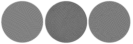
Figure 1: Images of domain chaos in Rayleigh-Bénard convection with $\Gamma=36$, $\varepsilon\equiv\Delta T/\Delta T_{c}-1=0.05$, and $\Omega=16.25$. Left: the temperature profile at the mid-plane from simulation of the Boussinesq equations with no centrifugal force. Center: shadowgraph image from experiment. A movie of this sample at $150\times$ actual speed is available MOV1 . Right: the temperature profile at the mid-plane from simulation of the Boussinesq equations including centrifugal force.

Domain chaos features patches of straight rolls oriented at various angles KL ; GK ; CB ; HB ; BH ; TC92 ; CMT94 ; HEA ; HEA2 ; HPAE . The orientation of the rolls fluctuates in time and space approximately at discrete angles due to the Coriolis force which induces the Küppers-Lortz instability. The size and shape of the domains also fluctuates and moving defects pepper the entire pattern creating a state of persistent chaos in both space and time. Figure 1 shows several snapshots of domain chaos.

The theoretical models that describe domain chaos usually neglect the centrifugal force, relying on the Coriolis force as the dominant effect brought by rotation. Even when the full Boussinesq equations of motion are considered, the centrifugal force often is evaluated on the assumption that the density is constant throughout the sample SC . In that case it has no influence on the neutral curve and on the pattern that forms above it. In this paper we show, both from experiment and from numerical simulations of the Boussinesq equations, that the centrifugal force does have a significant influence on the quantitative features of domain chaos. This is so even for modest aspect ratios $\Gamma\equiv r_{0}/d$, where $r_{0}$ and $d$ are the radius and height of the convection sample. When $\Gamma$ becomes large enough the centrifugal force qualitatively alters the observed patterns. In order to reproduce these features in the simulation, it is necessary to consider the temperature dependence of the density, as is done explicitly in the Appendix.

Qualitatively the influence of the centrifugal force is readily understood. The vertical density gradient, resulting from the imposed temperature difference, induces a radial large-scale circulation (LSC). The wave director of the RBC rolls tends to align orthogonally to the LSC CB91 . This tendency competes with the Küppers-Lortz mechanism that tends to create disordered and fluctuating domains.

For samples with $\Gamma$ up to about 40 we observed patterns in the experiment that were regarded as typical of domain chaos and similar to those found previously HEA ; HEA2 ; HPAE . However, as observed before HPAE , the patterns contained domains that were significantly smaller than those of simulations of the Boussinesq equations. At larger $\Gamma=80$ we found experimentally a hybrid state where the centrifugal force was strong enough relative to the Coriolis force to qualitatively affect the pattern as shown in Fig. 2. There the central section looked like domain chaos, but the annular region along the perimeter was mostly made up of nearly-stationary nearly-radial rolls. Defects glided azimuthally across the radial rolls (a movie of this state can be found in the online version). Although simulations of the Boussinesq equations for such large $\Gamma$ were not feasible, the inclusion of an enhanced centrifugal force in simulations for $\Gamma=20$ showed a similar radial roll structure near the sample boundary.

The outer region of the hybrid state had much in common with undulation chaos UC ; UC2 ; UC3 observed in inclined Rayleigh-Bénard convection. In the inclined system there is a component of gravity in the plane of the sample. The undulation chaos consists of defects gliding across straight rolls, with the roll axes aligned parallel to this in-plane component. Similarly, there is an alignment of the roll axes in the rotating case that is nearly parallel to the (radial) centrifugal force, with defects gliding azimuthally across the rolls. The resemblance between these phenomena exists in spite of the fact that these forces possess a very different character because the centrifugal force depends on radial position while gravity is uniform throughout the sample.

In the remainder of this paper we first give some experimental and theoretical/numerical details, and then present several results of quantitative pattern analysis that characterize the extent of the influence of the centrifugal force for $15\leq\Omega\leq 19$ ($\Omega\equiv\omega d^{2}/\nu$ where $\omega$ is the angular rotation rate and $\nu$ the kinematic viscosity) and $\varepsilon\equiv\Delta T/\Delta T_{c}-1\lesssim 0.5$. On the basis of this analysis we show for this parameter range that the crossover from the Coriolis-force-dominated central region of domain chaos to centrifugal-force-dominated near-radial rolls occurs near $r/d=35$ ($r$ is the radial coordinate) when $\varepsilon\gtrsim 0.1$, and at somewhat smaller $r/d$ for smaller $\varepsilon$. We conclude that previous samples had been too small to observe the qualitative features of the hybrid state. Unfortunately we also have to conclude that the experimental study of the Coriolis-force effect in compressed gases, where large aspect ratios are attainable, will be severely contaminated by centrifugal-force effects when $\Gamma\gtrsim 40$.

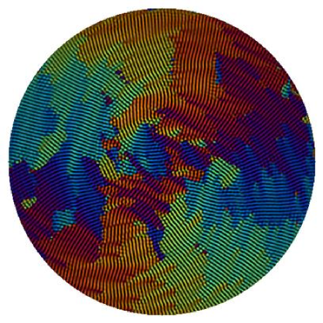
Figure 2: (Color online) Hybrid state of domain chaos with radial rolls and defects along the outer annulus. System parameters are $\Gamma=80$, $\varepsilon=0.05$, and $\Omega=16.25$. The grey-scale (false color in the electronic version) overlay is $\theta\left(\mathbf{r}\right)$, the angular component of the local wave-director field. A movie is available MOV2 showing the dynamics of this pattern at $150\times$ actual speed.

II Details of Experiment and Simulation

The sample exhibiting the large-$\Gamma$ hybrid state (see Fig. 2) had a height $d=553\leavevmode\nobreak\ \mu$m with $\Gamma=80$. It contained sulfur hexa-fluoride (SF₆) at a pressure of 25.44 bars and a mean temperature of $43.00^{\circ}\textrm{C}$ where the Prandtl number $\sigma\equiv\nu/\kappa$ was 0.88 ($\kappa$ is the thermal diffusivity). We used the shadowgraph technique to image the convection patterns in an apparatus described elsewhere EXP . Although Fig. 2 shows an image taken at $\Omega=16.25$, we observed a similar phenomenon over the entire range $15<\Omega<19$ of accessible rotation rates that were substantially above $\Omega_{c}$.

We also studied a medium and a small sample experimentally that did not exhibit the hybrid state. The medium sample had $\Gamma=61.5$, a thickness of 720$\mu$m, a pressure of 20.00 bars, a mean temperature of $38.00^{\circ}\textrm{C}$, and $\sigma=0.87$. The small sample had $\Gamma=36$, was 1230$\mu$m thick, operating at 12.34 bars, with a mean temperature of $38.00^{\circ}\textrm{C}$, and $\sigma=0.82$.

In addition to the experiment, we also simulated the Boussinesq equations to study the system theoretically. A discussion of the relevant equations of motion is given in the Appendix. Details of the numerical code are described elsewhere COMP1 ; SCHE . No-slip velocity boundary conditions and conducting lateral thermal boundary conditions were utilized. We used a spatial resolution of 0.1 and a time resolution of 0.005. In most simulations that included the centrifugal force, the centrifugal term was made larger than would be physically realistic, in the present experimental fluid, in order to model the effect of a larger aspect ratio.

Two different configurations were used to compute the precession frequency $f$. In one case, which included both the centrifugal and Coriolis force, we used $\Gamma=20$, $\sigma=0.93$, $\Omega=17.6$, and the centrifugal term was twice the physically realistic value in order to model a $\Gamma$ that would be twice as large. In the other case, where only the Coriolis force was included SCHE , we used $\Gamma=40$, $\sigma=0.93$, and $\Omega=17.6$. We compare the results of these simulations to the experimental results from Ref. HEA , which also used $\Gamma=40$, $\sigma=0.93$, and $\Omega=17.6$.

We also ran some simulations with the exact parameters of the $\Gamma=36$ experimental sample for direct comparison. Finally we ran several additional cases for the $\Gamma=20$ simulation using a centrifugal term with various strengths.

III Theoretical considerations

Although previous theoretical work on domain chaos TC92 ; KL ; GK ; CB ; HB ; BH ; CLM01 ; CMT94 ; PPS97 ; PPS97_2 ; LPPS neglected the centrifugal force because the Froude number $\textrm{Fr}\equiv\omega^{2}r/g$ ($g$ is the acceleration of gravity) is small in typical experiments, other research HH71 ; HART indicated that the Froude number may not be the only relevant parameter. Hart HART provided a numerical estimation of the parameter regimes where the centrifugal force is relevant. He made the approximation that $\Omega$ is large ($\gtrsim$ 500), so we cannot directly use that estimate because the present $\Omega$ values are only about 20. We instead consider

$${\cal A}=\frac{\beta\sigma\Omega\Gamma z_{0}}{2u_{0}\varepsilon^{1/2}}$$ (1)

($\beta\equiv\alpha\Delta T_{c}$ where $\alpha$ is the isobaric thermal expansion coefficient). A derivation of the relevant centrifugal and Coriolis terms is given in the Appendix. This parameter ${\cal A}$ is the small-$\varepsilon$ approximation to the ratio of the magnitude of the maximum of the centrifugal term, evaluated near the outer edge of the sample, to the magnitude of the Coriolis term evaluated where it reaches a maximum in the horizontal direction, $z=z_{0}$. (Note that the temperature of the conduction profile is equal to $-z$ for our system). The quantity ${\cal A}$ is an indicator of the transition from domain chaos to a hybrid state. We can obtain an approximate numerical value for $u_{0}$ by performing a linear stability analysis to get the functional form of the velocity and by using the simulation to get the normalization. For the case of $\Gamma=40$, $\sigma=0.93$ and $\Omega=17.6$, we find $u_{0}=12.3$ at $z_{0}=0.3$. These values should also approximately apply for our experimental parameters, which do not vary significantly from the parameters used to obtain the numerical values, except for $\Gamma$ whose dependence is explicit. For the $\Gamma=80$ sample, $\mathcal{A}=0.61$ for $\varepsilon=0.05$, indicating that the centrifugal force is almost as influential as the Coriolis force, but for the $\Gamma=36$ sample and $\varepsilon=0.05$, $\mathcal{A}=0.12$ indicating that the Coriolis force dominates. Both samples have similar values of $\Omega$ and $\sigma$, so it is not surprising that we observe a $\Gamma$-dependent transition to a hybrid state induced by competition between the centrifugal force and the Coriolis force.

IV Results

We qualitatively tested our hypothesis that the centrifugal force is responsible for the hybrid state by simulating the Boussinesq equations with centrifugal force included. It was not possible to reach $\Gamma=80$ in the simulation in order to directly reproduce Fig. 2. Instead we ran the simulation at $\Gamma=20$ and with the centrifugal force artificially large in order to model the stronger centrifugal force at larger $\Gamma$. Some results are shown in Fig. 3. The qualitative agreement between Fig. 2 and the right image of Fig. 3 is striking. Both exhibit domain chaos at the center but a radial roll structure in an annulus near the side wall.

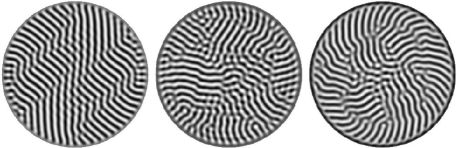
Figure 3: Simulation of the Boussinesq equations with $\Gamma=20$, $\sigma=0.93$, $\Omega=17.6$, $\varepsilon=0.055$, and an artificially large centrifugal force in order to model the effect of an inaccessibly large $\Gamma$. Left: zero centrifugal force. Center: centrifugal force is 4 times the physical value. Right: centrifugal force is 10 times the physical value. A movie of this sample at $100\times$ actual speed is available MOV3 .

In order to make a direct comparison with the experiment we also simulated the Boussinesq equations for $\Gamma=36$ at $\varepsilon=0.05$ with the exact parameters of the $\Gamma=36$ experimental sample, both with and without the centrifugal force included. Figure 1 compares examples of the resulting pattern between simulation, with and without the effect of centrifugal force, and experiment. As noted before HPAE , we observed that the domain size was too large when we neglected the centrifugal force as seen by comparing Figs. 1a and 1b. The domain size in patterns where we included the centrifugal force, as shown in Fig. 1c, qualitatively matched the experimentally observed shadowgraph image in Fig. 1b.

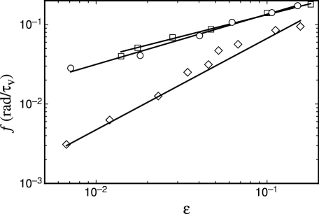
Figure 4: Effect of the centrifugal force on the scaling of the precession frequency $f$ with $\varepsilon$. All data are from samples with $\sigma=0.93$ and $\Omega=17.6$. Circles: from simulations that include both the centrifugal force and the Coriolis force, with $\Gamma=20$ and a centrifugal term that is twice as large as it would be in the experimental fluid. Diamonds: from simulations that include only the Coriolis force, with $\Gamma=40$. Squares: data from previous experiments, with $\Gamma=40$ HEA . Solid lines: least-squares fits of $f=C\varepsilon^{\mu}$ to the data.

Recent experiments HEA disagreed with the theoretical prediction TC92 ; CMT94 $\xi\sim\varepsilon^{-1/2}$ for the scaling of the correlation length $\xi$ and $f\sim\varepsilon^{\mu}$ with $\mu=1$ for the scaling of the domain precession frequency $f$. We do not address the $\xi$ scaling in the present work because finite-size effects cloud the issue CLM01 ; BA05 . However, $\mu$ is unaffected by the finite-size effects CLM01 ; BA05 . The method of determining $f$ is discussed in Refs. HEA ; SCHE . We find that $f$ from the experiment agrees with the simulation when the centrifugal force is included. The scaling for $f$ is shown in Fig. 4 for simulations both with and without the centrifugal force. The simulations that neglected the centrifugal force gave a scaling exponent $\mu=1.15$, in good agreement with the prediction of $\mu=1$ from amplitude equations TC92 which also neglected the centrifugal force. There is also good agreement between the experimental data and the results of the simulation where both the centrifugal and Coriolis force were included. Not only did the numerical simulation yield a scaling exponent of $\mu=0.62$, very close to $\mu=0.58$ from the experiment, but it also reproduced the actual values of $f$ in the experiment remarkably well.

Aside from the dramatic effect on the pattern seen in Fig. 2, in the experiment we also observed a downward shift by three or four percent of the critical Rayleigh number $R_{c}=\alpha g\Delta T_{c}d^{3}/\kappa\nu$ for the large sample. Previous work HH71 ; HART showed that the centrifugal force may either stabilize or destabilize the convective flow depending on the parameter regime, although the range of parameters specifically corresponding to the present case was not directly investigated. However it was suggested that for small $\Omega$ the centrifugal force lowers $R_{c}$ HART .

We did not observe any radial dependence of $R_{c}$ for the $\Gamma=80$ sample. We measured $R_{c}$ in both a central circular region of half the sample radius and in the outer annulus surrounding that region. We accomplished this by computing the time averaged total power in the specified region of the experimental images as a function of $\Delta T$. The total power is proportional to $\mathcal{N}-1$ where $\mathcal{N}$ is the Nusselt number. Through a quadratic fit we extrapolated to the background value of the total power in order to measure $\Delta T_{c}$, from which we calculated $R_{c}$ from knowledge of the fluid properties. The values for $R_{c}$ in both regions agreed within the statistical error of the data, with the biggest difference being a bit less than 0.2%, i.e. an order of magnitude less that the down shift of $R_{c}$.

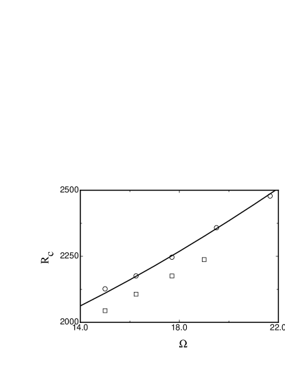
Figure 5: Shifted critical Rayleigh number due to the centrifugal force. Solid line: prediction from linear stability analysis. Circles: measured from the $\Gamma=61.5$ sample. Squares: measured from the $\Gamma=80$ sample.

The linear stability analysis SC for this system was carried out for a laterally infinite system using the Coriolis force only and neglecting the centrifugal force. For $\Gamma=61.5$, our measured $R_{c}$ agreed well with this analysis as is seen in Fig. 5. Similarly good agreement had been found earlier for $\Gamma=40$ HEA2 . This is interesting because we do observe other centrifugal effects for $\Gamma=61.5$, as discussed below. For $\Gamma=80$ there was a clear downward shift of $R_{c}$, relative to the theory and to experiments for smaller $\Gamma$, of roughly 3%. This trend with $\Gamma$ indicates that the disagreement with theory cannot be attributed to the finite size of the experimental systems because any finite-size effect on the onset should have been larger at smaller $\Gamma$. Thus it suggests that for $\Gamma=80$ the centrifugal force, which increases with increasing $\Gamma$, has become strong enough to affect the onset.

We quantified our analysis of the experimental images by utilizing the angular component $\theta\left(\mathbf{r}\right)$ of the local wave-director field computed with an algorithm described in Ref. CMT94 , but using higher angular resolution. Figure 2 shows an example of $\theta\left(\mathbf{r}\right)$ overlayed on top of the shadowgraph pattern in false color. We used the variance field of $\theta\left(\mathbf{r}\right)$, from a time series of consecutive images, to address the issue of which region of the pattern exhibits chaotic dynamics and which region is mostly dominated by near-stationary radial rolls. Chaotic patterns exhibit a large variance because the roll orientation fluctuates constantly, but stationary rolls yield a small variance.

The mean angular sum field is

$$S\left(\mathbf{r}\right)=\sum_{n}^{N}e^{2i\theta_{n}\left(\mathbf{r}\right)}$$ (2)

where $n$ is the image index and $N$ is the number of images. The complex exponential introduces the necessary periodicity for summing angles and the factor of 2 treats the field as a director field instead of as a vector field. The mean angular field is

$$\overline{\theta}\left(\mathbf{r}\right)=\frac{1}{2}\arctan\left(\frac{\textrm{Im}S}{\textrm{Re}S}\right)\textrm{.}$$ (3)

The angular variance field is

$$\left\langle\theta^{2}\right\rangle\left(\mathbf{r}\right)=\frac{1}{N}\sum_{n}^{N}\left|e^{2i\theta_{n}\left(\mathbf{r}\right)}-e^{2i\overline{\theta}\left(\mathbf{r}\right)}\right|\textrm{.}$$ (4)

Simple algebra shows that $0\leq\left\langle\theta^{2}\right\rangle\left(\mathbf{r}\right)\leq 2$ where a value of 0 indicates that the domain orientation is stationary while a value of 2 indicates that it is maximally fluctuating. The variance field $\left\langle\theta^{2}\right\rangle\left(\mathbf{r}\right)$ is approximately azimuthally symmetric for several investigated system sizes as shown in Fig. 6. There one sees for the larger two samples that the variance is large near the center and smaller near the side wall.

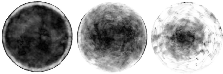
Figure 6: The variance field $\left\langle\theta^{2}\right\rangle\left(\mathbf{r}\right)$ for several system sizes from experiment with $\varepsilon=0.05$ and $\Omega=16.25$. Black corresponds to $\left\langle\theta^{2}\right\rangle\left(\mathbf{r}\right)=2$ and white corresponds to $\left\langle\theta^{2}\right\rangle\left(\mathbf{r}\right)=0$. Left: $\Gamma=36$. Middle: $\Gamma=61.5$. Right: $\Gamma=80$

Figure 7 displays $\left\langle\theta^{2}\right\rangle\left(r\right)$, the azimuthal average of the angular variance field, for several system sizes. For the smallest experimental sample and for a simulation with matching parameters, both with $\Gamma=36$, the large variance across the entire sample revealed the presence of domain chaos throughout. However, as seen in Fig. 1, even in this case the centrifugal force has reduced the domain size. Likewise, the central region of the largest sample, with $\Gamma=80$, exhibited a large variance. Domain chaos dominated near this central region, but along the perimeter of the sample the variance was very small indicating coexistence with a more nearly stationary pattern. The variance for both the $\Gamma=61.5$ and $\Gamma=80$ samples showed a clear crossover from domain chaos to radial rolls, however the $\Gamma=61.5$ sample did not fully transition out of domain chaos even at the edge of the sample.

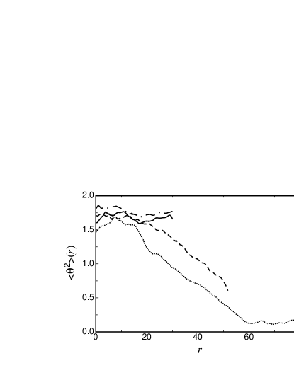
Figure 7: Azimuthal average $\left\langle\theta^{2}\right\rangle\left(r\right)$ of the angular variance field (shown in Fig. 6) for various system sizes from both experiment and simulation. All data were taken with $\varepsilon=0.05$ and $\Omega=16.25$. Solid line: experiment, $\Gamma=36$. Dashed line: experiment, $\Gamma=61.5$. Dotted line: experiment, $\Gamma=80$. Dashed-dotted line: simulation including centrifugal force, $\Gamma=36$.

We also measured the size of the domain chaos region of the hybrid state by finding the width $b$ of $\left\langle\theta^{2}\right\rangle\left(r\right)$ chosen such that $\left\langle\theta^{2}\right\rangle\left(b\right)\equiv\left\langle\theta^{2}\right\rangle\left(0\right)/2$. Figure 8 shows the $\varepsilon$ dependence of $b$. The behavior of $\mathcal{A}$ (see Eq. 1) at small $\varepsilon$ agrees with such $\varepsilon$ dependence because of the factor $\varepsilon^{1/2}$ in the denominator, associated with the Coriolis force, which gives $\mathcal{A}\sim\varepsilon^{-1/2}$ for small $\varepsilon$. The data in Fig. 8 indicate that, for the present sample parameters, the centrifugal force dominates at small $\varepsilon$ while the Coriolis force becomes more important at large $\varepsilon$, although for large enough $\Gamma$ neither are negligible.

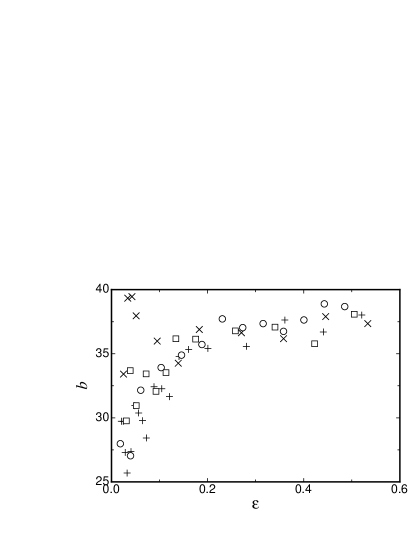
Figure 8: Width $b$ of $\left\langle\theta^{2}\right\rangle\left(r\right)$ for $\Gamma=80$ at various $\varepsilon$. Crosses: $\Omega=15$. Circles: $\Omega=16.25$. Squares: $\Omega=17.7$. Pluses: $\Omega=19$.

In addition to looking at the fluctuations in the wave-director angle, we also measured the angle of the wave director relative to the angle $\theta_{\hat{r}}$ of the side-wall normal by computing a time-averaged dot-product-like quantity

$$D\left(\mathbf{r}\right)=\frac{1}{N}\sum_{n}^{N}\cos 2\left[\theta_{\hat{r}}-\theta\left(\mathbf{r}\right)\right]\ .$$ (5)

Here we are using $\theta_{\hat{r}}$ as a reference for the orientation of the centrifugal force. The quantity $D\left(\mathbf{r}\right)$ is 1 when the wave director is parallel to the sidewall normal and -1 when it is perpendicular.

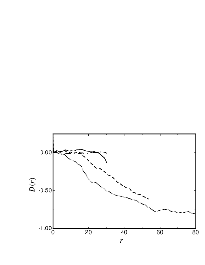
Figure 9: The time-averaged dot product $D\left(r\right)$ (the azimuthal average of $D\left(\mathbf{r}\right)$) for the same data as shown in Fig. 7. All data were taken with $\varepsilon=0.05$ and $\Omega=16.25$. Solid line: experiment, $\Gamma=36$. Dashed line: experiment, $\Gamma=61.5$. Dotted line: experiment, $\Gamma=80$. Dashed-dotted line: simulation including centrifugal force, $\Gamma=36$.

In the presence of the LSC induced by the centrifugal force, we expect the wave director to line up nearly perpendicular to that flow CB91 . Some deviation from this might be expected due to the action of the Coriolis force on the Rayleigh-Bénard rolls. The LSC itself would be expected to nearly align with the centrifugal force and thus should be nearly orthogonal to the side wall. However, here also some deviation from orthogonality to the walls would be expected due to the Coriolis-force influence. As expected, Fig. 9 shows that, as $\Gamma$ increases, the wave director along the edge of the sample indeed does become more nearly, but not perfectly, perpendicular to the sidewall normal. For the largest $\Gamma$, $D\left(r\right)$ reached a plateau around -0.8, which corresponded to an angle of about $74^{\circ}$, somewhat shy of a perpendicular angle.

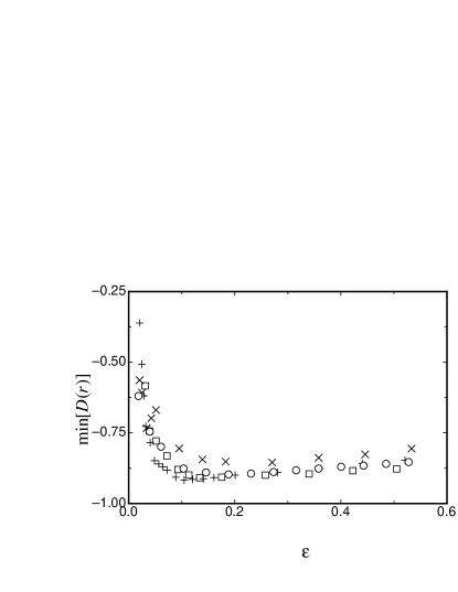
Figure 10: Average minimum $D\left(r\right)$ for $\Gamma=80$ at various $\varepsilon$. Crosses: $\Omega=15$. Circles: $\Omega=16.25$. Squares: $\Omega=17.7$. Pluses: $\Omega=19$.

The angle also depended on $\varepsilon$ as indicated by Fig. 10, which shows the minimum value of $D\left(r\right)$ for many curves similar to those shown in Fig. 9. To reduce the effect of statistical fluctuation in the $D\left(r\right)$ curves, the plateau in those curves was averaged over a small radial length of roughly $5d$ to yield an average minimum value for $D\left(r\right)$, $\textrm{min}\left[D\left(r\right)\right]$, at the given $\varepsilon$ and $\Omega$. As a function of $\varepsilon$, $\textrm{min}\left[D\left(r\right)\right]$ exhibited a minimum, between $\varepsilon=0.1$ and $\varepsilon=0.3$ depending on $\Omega$, which corresponded to the nearest realization of orthogonality between the sidewall normal and the wave-director. For small $\varepsilon$ the rolls started to turn in and become nearer to concentric rings along the outer annulus. Such behavior is indicative of the $\varepsilon$ dependence of the relative strengths of the centrifugal and Coriolis forces.

We also compared auto-correlation functions of the wave-director field between the experiment and simulation. Using $\theta\left(\mathbf{r}\right)$ we computed

$$C\left(\delta\mathbf{r}\right)=\frac{1}{M\left(\delta\mathbf{r}\right)}\int\cos 2\left[\theta\left(\mathbf{r}\right)-\theta\left(\mathbf{r}+\delta\mathbf{r}\right)\right]d\mathbf{r}$$ (6)

which is slightly different from the formula used in Ref. CMT94 . The difference is the inclusion of a factor $M\left(\delta\mathbf{r}\right)$, the number of data points integrated over to find the correlation at the coordinate $\delta\mathbf{r}$, which corrects for the diminished quantity of data available at increasingly separated correlations. This correction results in what is known as an unbiased correlation function, as opposed to the biased correlation function given when $M\left(\delta\mathbf{r}\right)=1$. Both approaches have merits, in particular the biased form must be used for computing power spectra, but we prefer the unbiased form in the present case.

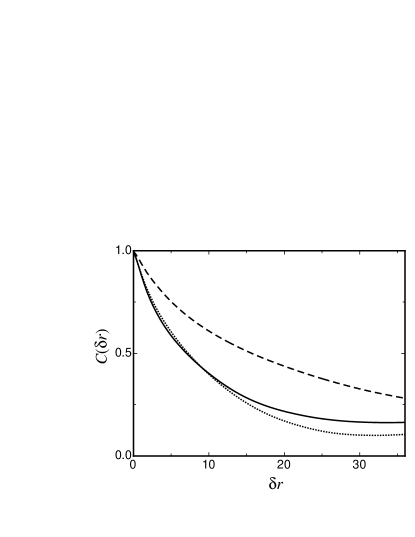
Figure 11: Azimuthal average of the auto-correlation function of the wave-director angle field for $\Gamma=36$, $\varepsilon=0.05$, $\Omega=16.25$, $\sigma=0.82$. Solid line: from simulation of Boussinesq equations with centrifugal force included. Dashed line: from simulation but with centrifugal force neglected. Dotted line: from experiment.

The angular auto-correlation function magnifies the difference between centrifugal force and lack of centrifugal force as shown in Fig. 11. The agreement between the experiment and the full simulation with centrifugal force was excellent at small and moderate $\delta r$, and indicated a quantitative agreement of the domain size between experiment and simulation with centrifugal force, as observed qualitatively in Fig. 1. The slight deviation at large separations should probably be disregarded due to lack of a sufficient quantity of data, even with the help of the unbiased form of the auto-correlation function to mitigate this issue. The simulation which neglected centrifugal force exhibited an overall larger correlation than the experimental result, in agreement with the larger domains shown in Fig. 1.

V Summary and Conclusion

We have shown that the centrifugal force plays an important role in the domain chaos state of Rayleigh-Bénard convection. Even for relatively small $\Gamma$ where $\mathcal{A}$ remains small throughout the sample, the centrifugal force affects both the pattern domain size and also the precession frequency. At large enough $\Gamma$, a hybrid state forms that contains both domain chaos and radial patterns reminiscent of undulation chaos. We have characterized this hybrid state using local wave-director analysis. We also observed a slight shift in $R_{c}$ for this state.

Comparison between simulations and experiment at moderate $\Gamma$ indicated that the centrifugal force is responsible for the disagreement of previous experiment with the scaling $f\sim\varepsilon$ predicted by the amplitude model for domain chaos. A simulation which neglected centrifugal force agreed with that model, but a simulation which included centrifugal force agreed with the experiment.

Appendix A Rotational Corrections to the Boussinesq Equations

We begin with the Navier-Stokes equation in a rotating frame and in the presence of gravity, the heat equation and mass conservation:

$$\left(\partial_{t}+\mathbf{u}\cdot\nabla\right)\mathbf{u} = -{\nabla P\over\rho}+\nu\nabla^{2}\mathbf{u}-g\hat{z}-2\,\omega\,\hat{z}\times\mathbf{u}+\omega^{2}\mathbf{r},$$

$$\left(\partial_{t}+\mathbf{u}\cdot\nabla\right)T = \kappa\nabla^{2}T,$$

$$\nabla\cdot\mathbf{u} = 0,$$

where $\mathbf{u}$ is the velocity field, $T$ is the temperature field, $P$ is the pressure field.

We apply the Boussinesq approximation, in which all fluid parameters are assumed to be constant except for the density in the buoyancy term. Unlike the standard application of this approximation SC , we include buoyancy from the centrifugal force as well as gravity. To lowest order, the density variation in these terms is

$$\rho=\bar{\rho}[1-\alpha(T-\bar{T})],$$ (8)

where $\bar{T}$ is the mean temperature and $\bar{\rho}$ is the density at that temperature.

As long as $\alpha(T-\bar{T})$ is small, we can expand the pressure term:

$$-{\nabla P\over\rho}\simeq-{\nabla P\over\bar{\rho}}[1+\alpha(T-\bar{T})].$$ (9)

Since the pressure is determined from a gradient, we can absorb the hydrostatic pressure due to the gravitational and the centrifugal forces into the dynamic pressure, by redefining $P=P+\bar{\rho}gz\hat{z}-{\bar{\rho}\over 2}\omega^{2}(x^{2}\hat{x}+y^{2}\hat{y})$. The terms proportional to the temperature will not be absorbed. Equation (LABEL:navstodim) becomes:

$$\left(\partial_{t}+\mathbf{u}\cdot\nabla\right)\mathbf{u} = -{\nabla P\over\bar{\rho}}+\nu\nabla^{2}\mathbf{u}+g\alpha(T-\bar{T})\hat{z}$$ (10)

$$- 2\,\omega\,\hat{z}\times\mathbf{u}-\omega^{2}\alpha(T-\bar{T})\mathbf{r},$$

where we have assumed the term $\nabla P\alpha(T-\bar{T})/\bar{\rho}$ is small.

The variables are then non-dimensionalized by specifying the length in terms of the cell height $d$, the temperature in terms of $\Delta T$, and the time in units of the vertical thermal diffusion time $\tau_{v}=d^{2}/\kappa$. We also define the Prandtl number $\sigma=\nu/\kappa$, and the Rayleigh number $R=\alpha g\Delta Td^{3}/\kappa\nu$. In addition, we define $\beta=\alpha\Delta T_{c}$, where $\Delta T_{c}$ (and corresponding critical Rayleigh number $R_{c}$) is the temperature difference at which conduction gives way to convection. We obtain:

$$\sigma^{-1}\left(\partial_{t}+\mathbf{u}\cdot\nabla\right)\mathbf{u} = -{\nabla P}+\nabla^{2}\mathbf{u}+R(T-\bar{T})\hat{z}$$

$$- 2\Omega\hat{z}\times\mathbf{u}-\beta\sigma\Omega^{2}{R\over R_{c}}(T-\bar{T})\mathbf{r},$$

$$\left(\partial_{t}+\mathbf{u}\cdot\nabla\right)T = \nabla^{2}T,$$

$$\nabla\cdot\mathbf{u} = 0.$$

The ratio of the magnitude of the centrifugal term to the magnitude of the Coriolis term is evaluated at the position where the Coriolis force reaches its maximum value, which is where the magnitude of horizontal velocity $u_{\perp}$ is a maximum. To first order in $\varepsilon^{1/2}$ we can define this magnitude $|u_{\perp}|=u_{0}\varepsilon^{1/2}$, which occurs at $z=z_{0}$. At this point, the absolute value of $T-\bar{T}$ = $z_{0}$, the temperature due to the conduction profile. (Note we have neglected convective corrections to the conduction profile, since these are of order $\varepsilon^{1/2}$). We also want to evaluate the centrifugal force at the horizontal location where it reaches its maximum value, which is at $r=\Gamma$, which then yields Eq. 1.

References

- (1) S. Chandrasekhar, Hydrodynamic and Hydromagnetic Stability, (Oxford University Press, Oxford, 1961).
- (2) For a review, see for instance E. Bodenschatz, W. Pesch, and G. Ahlers, Annu. Rev. Fluid Mech. 32, 709 (2000).
- (3) G. Küppers and D. Lortz, J. Fluid Mech. 35, 609 (1969).
- (4) G. Küppers, Phys. Lett. 32A, 7 (1970).
- (5) R.M. Clever and F.H. Busse, J. Fluid Mech. 94, 609 (1979).
- (6) K.E. Heikes and F.H. Busse, Ann. N.Y. Acad. Sci. 357, 28 (1980).
- (7) F.H. Busse and K.E. Heikes, Science 208, 173 (1980).
- (8) Y. Tu and M. Cross, Phys. Rev. Lett. 69, 2515 (1992).
- (9) M. Cross, D. Meiron, and Y. Tu, Chaos 4, 607 (1994).
- (10) Y.-C. Hu, R.E. Ecke, and G. Ahlers, Phys. Rev. Lett. 74, 5040 (1995).
- (11) Y.-C. Hu, R.E. Ecke, and G. Ahlers, Phys. Rev. E 55, 6928 (1997).
- (12) Y.-C. Hu, W. Pesch, G. Ahlers, and R.E. Ecke, Phys. Rev. E 58, 5821 (1998).
- (13) See EPAPS Document No. ??? for an MPEG movie of Fig. 1b with a color overlay of . This document can be reached via a direct link in the online article’s HTML reference section or via the EPAPS homepage (http://www.aip.org/pubservs/epaps.html).
- (14) R.M. Clever and F.H. Busse, J. Fluid Mech. 229, 517 (1991).
- (15) K.E. Daniels, B.P. Plapp, and E. Bodenschatz, Phys. Rev. Lett. 84, 5320 (2000).
- (16) K.E. Daniels and E. Bodenschatz, Phys. Rev. Lett. 88, 034501 (2002).
- (17) K.E. Daniels and E. Bodenschatz, Chaos 13, 55 (2003).
- (18) J.R. deBruyn, E. Bodenschatz, S. Morris, S. Trainoff, Y.-C. Hu, D.S. Cannell, and G. Ahlers, Rev. Sci. Instrum. 67, 2043 (1996).
- (19) See EPAPS Document No. ??? for an MPEG movie of Fig. 2. This document can be reached via a direct link in the online article’s HTML reference section or via the EPAPS homepage (http://www.aip.org/pubservs/epaps.html).
- (20) P. F. Fischer, J. Comp. Phys. 133, 84 (1997).
- (21) J.D. Scheel and M.C. Cross, Phys. Rev. E, in print.
- (22) M.C. Cross, M. Louie, and D. Meiron, Phys. Rev. E63, 45201 (2001).
- (23) Y. Ponty, T. Passot, and P. Sulem, Phys. Rev. Lett. 79, 71 (1997).
- (24) Y. Ponty, T. Passot, and P. Sulem, Phys. Rev. E 56, 4162 (1997).
- (25) D. Laveder, T. Passot, Y. Ponty, and P. L. Sulem, Phys. Rev. E 59, R4745 (1999).
- (26) G.M. Homsy and J.L. Hudson, J. Fluid Mech. 48, 605 (1971).
- (27) J.E. Hart, J. Fluid Mech. 403, 133 (2000).
- (28) See EPAPS Document No. ??? for an MPEG movie of Fig. 3c. This document can be reached via a direct link in the online article’s HTML reference section or via the EPAPS homepage (http://www.aip.org/pubservs/epaps.html).
- (29) N. Becker and G. Ahlers, unpublished.