STICKINESS OF TRAJECTORIES IN A PERTURBED ANOSOV SYSTEM

G.M. Zaslavsky^(1,2) and M. Edelman^(1)
(1)Courant Institute of Mathematical Sciences, New York University, 251 Mercer St., New York, NY 10012, USA
⁽²⁾Department of Physics, New York University, 2-4 Washington Place, New York, NY 10003, USA
Email: zaslav@cims.nyu.edu
Email: edelman@cims.nyu.edu

Abstract

We consider a perturbation of the Anosov-type system, which leads to the appearance of a hierarchical set of islands-around-islands. We demonstrate by simulation that the boundaries of the islands are sticky to trajectories. This phenomenon leads to the distribution of Poincaré recurrences with power-like tails in contrast to the exponential distribution in the Anosov-type systems.

1. INTRODUCTION

Anosov maps (or Anosov-type maps, or Anosov diffeomorphisms) can be considered as a strong idealization of realistic systems. The reason of this is that Hamiltonian systems are not uniformly hyperbolic and their phase space features a complex mixture of zones of different dynamics. The boundaries of the zones influence the trajectories and drastically change asymptotic properties of transport. The ways how the Anosov systems can lose their hyperbolicity is the subject of various investigations [1, 2, 3, 4, 5]. The main questions discussed here are a description of the topological pattern of the destroyed hyperbolicity and the description of the consequences of that loss. For the latter issue, it could be, for example, the changes in particles transport due to the changes in the phase space topology that occurs in Hamiltonian systems with mixed phase space [6], i.e. phase space with chaotic sea and islands.

In this paper we make few comments related to the destruction of hyperbolicity and to the problem of transport. The considered system is similar to the introduced one in [1]. It is a map that acts on the torus ${\bf T}^{2}$ and it depends on an intrinsic parameter $K\in(-\infty,\infty)$, and on the perturbation parameter $\epsilon_{0}$. The uniform hyperbolicity exists when $\epsilon_{0}=0$ and in a region ${\bf K}_{+}$ of the values of $K$. The system is most sensitive to the perturbation in the vicinity of edges of ${\bf K}_{+}$. In the extended space ${\bf T}^{2}\times{\bf K}$ the system is unstable with respect to an arbitrary small $\epsilon_{0}$. Increasing $\epsilon_{0}$ leads to a sequence of bifurcations. We demonstrate by simulations the appearance of a hierarchical set of islands in the stochastic sea and a stickiness of their borders. In other words, trajectories spend enormously long time in the vicinity of the islands’ border making the transport to be anomalous. The “anomalous” means that the wandering of trajectories strongly differs from the random walk in the case of uniform hyperbolicity. This property is established numerically by applying the method of $\epsilon$-separation along reference trajectories developed in [7, 8, 9]. The main result can be expressed in a simplified form as follows: After the loss of hyperbolicity, the considered Anosov system reveals the power law of the distribution of Poincaré recurrences when $t$ (time) $\rightarrow\infty$, in contrast to the exponential distribution for unperturbed Anosov system [10].

2. DESCRIPTION OF THE SYSTEM

Consider a dynamical system $(x,y)\in{\bf T}^{2}$ defined on the two-dimensional torus by the equation of motion

$$y_{n+1}=y_{n}+f(x_{n};\epsilon_{0},K);\ \ \ \ x_{n+1}=x_{n}+y_{n+1}\ ,\ \ \ \ ({\rm modd}\ 1)$$ (1)

and a differentiable function

$$f(x_{n};\epsilon_{0},K)=Kx_{n}-\epsilon_{0}\psi(x_{n})$$ (2)

with two parameters $K$ and $\epsilon_{0}$. The map (1) is area-preserving for any $f(x;\epsilon_{0},K)$. While the map acts in the phase space which is $\mathord{\mbox{\boldmath$T$}^{2}}$, it doesn’t transform the boundary of the torus $\partial\mathord{\mbox{\boldmath$T$}^{2}}$ into $\partial\mathord{\mbox{\boldmath$T$}^{2}}$. Particularly, for $\epsilon_{0}=0$ it is evident since $K$ is not integer. This is a typical physical situation. One can interpret the map (1) as a generator of trajectories $\{x_{0},y_{0};x_{1},y_{1};...\}$ in the lifted space $(x,y)\in(-\infty,\infty;-\infty,\infty)$, which should be, afterward, bended and put inside the compact phase space $(x,y)$ $modd1$. This way of the consideration of the map (1) permits to study infinite diffusion in the lifted space and local measures, Poincaré recurrences measure, etc. in the phase space $T^{2}=(x,y)$ $modd1$.

The eigenvalues of the tangent to (1) map are

$$\lambda_{1,2}=\left(1+{1\over 2}K-{1\over 2}\epsilon_{0}\psi^{\prime}(x)\right)\pm\left[\left(1+{1\over 2}K-{1\over 2}\epsilon_{0}\psi^{\prime}(x)\right)^{2}-1\right]^{1/2}\ .$$ (3)

For $\epsilon_{0}=0$ the region

$${\bf K}_{+}:\ K<-4\ ,\ \ \ K>0\ ;\ \ \ \ (\epsilon_{0}=0)$$ (4)

corresponds to uniformly hyperbolic dynamics, and the region

$${\bf K}_{-}:\ -4<K<0$$ (5)

corresponds to periodic dynamics with zero Lyapunov exponent. For our following consideration a specific form of $\psi(x)$ is not so important. Nevertheless, we specify it for a convenience

$$\psi(x)=\sin x\cdot\cos^{2}x\ ,$$ (6)

as it was considered in [1, 4].

The system (1), (2) represents Anosov diffeomorphism for $\epsilon_{0}=0$, $K\in{\bf K}_{+}$, and it is structurally (topologically) stable for $\epsilon_{0}\rightarrow 0$. Our goal is to consider structural stability in the extended space ${\bf T}^{2}\times{\bf K}$ where $K\in{\bf K}$.

3. ISLANDS AND ISLANDS HIERARCHY

Property 1. For arbitrary small $\epsilon_{0}$ there exists $K^{\pm}_{\epsilon_{0}}\in{\bf K}$ such that for $K\in(K^{-}_{\epsilon_{0}},K^{+}_{\epsilon_{0}})$ phase space ${\bf T}^{2}$ has islands of periodic orbits that appear as a result of the bifurcation. The main reason for this is that the hyperbolicity has edges defined in (4), (5 and arbitrary small $\epsilon_{0}$ influence the system’s stability fairly close to the edges. An example of the island born is in Fig. 1. For $\epsilon_{0}\neq 0$ the domain of stability

$${\bf K}_{-}:\ -4+\epsilon_{0}\psi^{\prime}(x)<K<\epsilon_{0}\psi^{\prime}(x)$$ (7)

depends on $x$, and the phase space becomes non-uniform.

Figure 1: Poincaré map of a trajectory for the system (1) with (2), (6) and $K=0.2$, $\epsilon_{0}=0.2$ (left), $\epsilon_{0}=0.16$ (right).

For small $\epsilon_{0}$ the most interesting domain is near $x=0$ and small $K$. For small $x$ we have from (2):

$$f(x)=\delta x+(7/6)\epsilon_{0}x^{3}+O(x^{3})\ ;\ \ \ \delta=K-\epsilon_{0}\ .$$ (8)

The map ( (1), in the vicinity of (0,0), gives for $\delta\rightarrow 0$

$$y_{n+2}=(1+\delta)y_{n}+2\delta x_{n}+{7\over 6}\epsilon_{0}x_{n}^{3}+O(\delta^{2})$$

$$x_{n+2}=(1+3\delta)x_{n}+2y_{n}+{7\over 3}\epsilon_{0}x_{n}^{3}+O(\delta^{2})$$ (9)

that is area-preserving up to the terms of the order $\delta^{3/2}$, $\delta x$. On the same level of accuracy, the map (9) can be written as Hamiltonian equations

$$\dot{y}=-{\partial H\over\partial x}\ ,\ \ \ \ \dot{x}=-{\partial H\over\partial y}\ ,$$

$$H\approx-{1\over 2}\delta x^{2}+{1\over 2}y^{2}+O(|\delta|^{3/2})$$ (10)

$$\dot{y}\approx{1\over 2}(y_{n+2}-y_{n})\ ,\ \ \ \ \dot{x}\approx{1\over 2}(x_{n+2}-x_{n})\ .$$

These expressions can be easily improved to have terms of higher order but we will not need it. An elliptic island appears around the point $x=y=0$ for $\delta<0$, i.e. for $K<\epsilon_{0}$ in correspondence to (7) and (6). The island has a scaling

$$y\sim|\delta|^{1/2}x\ ,\ \ \ \ (\delta\rightarrow 0)$$ (11)

Figure 2: Sticky islands for the same equation as in Fig. 1 with $K=K^{*}=1$ and $\epsilon_{0}=\epsilon_{0}^{*}=1.689538$. (a) full phase space; (b) zoom of the group of islands on the top right of (a); (c) zoom of a next generation island from the left island of (b); (d) zoom of the lower island in (c).

The value $\delta=0$ is the point of degeneracy and the bifurcation “opens” an island in the phase space [4]. Increasing of $|\delta|$ leads to a sequence of bifurcations that change the phase space topology. A particular case, shown in Fig. 2, is of special interest. For the specific values of the pair $(K,\epsilon)$ we have a hierarchical structure of islands-around-islands with a sequence of islands: $1-4-4\cdot 3-4\cdot 3\cdot 8-4\cdot 3\cdot 8\cdot 8-4\cdot 3\cdot 8\cdot 8\cdot 8-\ldots$. The values

$$(K^{*},\epsilon^{*}):\ K^{*}=1\ ,\ \ \ \ \epsilon_{0}^{*}=1.689538\ldots$$ (12)

are found numerically, for which the hierarchy of islands has a constant asymptotic proliferation number 8. Sequences of islands with bounded values of $m_{j}:\ m_{j}\in(m^{-},m^{+})$ is called a hierarchy of islands since the full number of islands at the hierarchy level $n$ is equal $\bar{m}^{n}$ with some $\bar{m}\in(m^{-},m^{+})$ and $n\rightarrow\infty$.

Property 2. There exists an infinite number of hierarchy of islands sequences $(1,m_{1},m_{2},\ldots)$ and the corresponding pairs $(K,\epsilon_{0})$. For a fixed $\epsilon$ (or $K$), it was assumed in [11] (see also [6]), that the values of $K$ (or $\epsilon_{0}$) to have an island hierarchy, are at least as dense as rationals. Many examples of this type of islands topology can be found in the review [6].

4. STICKINESS AND QUASI-TRAPS

The phenomenon of a long time stay of particles in the vicinity of the islands border is called stickiness. While it is known that the stickiness is due to the presence of cantori and some renormalization group approach can be applied to study particles transport through the cantori [12], a rigorous theory of stickiness does not exist yet and many features of the stickiness are waiting for our understanding (see more in [6]). A definition of stickiness can be provided using the notion of dynamical traps[13], or for Hamiltonian systems, quasi-traps.

Let $\Gamma$ be the compact phase space of a dynamical system that is Hamiltonian and chaotic in a part of $\Gamma$, and let $\Gamma_{A}\subset\Gamma$ be an island imbedded in the stochastic sea. Consider a border of the island, $\partial\Gamma_{A}$, and an annulus ${\bf A}=\partial\Gamma_{A}\times{\bf L}$ with a fairly small width $\ell$. For any initial condition $(x,y)\in{\bf A}$, one can consider a time $\tau(x,y;{\bf A})$ of a trajectory first exit from $\bf A$. This time is non-zero and non-infinite, since the dynamics is area-preserving.

The function $\rho(\tau;{\bf A})$ is called a distribution function of the trapping or escape time from the domain ${\bf A}$ if

$$\Psi(t;{\bf A})=\int_{t}^{\infty}d\tau\rho(\tau;{\bf A})=1-\int_{0}^{t}d\tau\rho(\tau;{\bf A})$$ (13)

is the probability to escape from ${\bf A}$ after time $\geq t$. Consider moments

$$\langle\tau^{q}\rangle_{A}=\int_{0}^{\infty}d\tau\ \tau^{q}\rho(t;{\bf A})\ .$$ (14)

For $q=1$ we have $\langle\tau\rangle_{A}<\infty$ due to the Kac lemma [14], i.e. the mean trapping time is finite. The domain $\bf A$ is called quasi-traps if there exists such $q>1$ that $\langle\tau^{q}\rangle_{A}=\infty$ [13, 6]. Evidently the distribution function $\rho(t;{\bf A})$ should satisfy the condition

$$\rho(t;{\bf A})\sim 1/t^{\gamma}\ ,\ \ \ \gamma>1\ ,\ \ \ \ (t\rightarrow\infty)\ ,$$ (15)

for quasi-traps.

There are many examples of systems with quasi-traps: standard map, Sinai and Bunimovich billiards (with $\gamma\approx 3$), rhombic billiard (with, most probably, $\gamma$ close to 2), and others (see in review [6]). It was assumed in [6] that realistic Hamiltonian systems with a hierarchy of islands reveals the dynamics with quasi-traps. In this paper we demonstrate by simulations that similar property exists for the perturbed Anosov diffeomorphism (1), (2) near the point (12) where a hierarchy of islands appears.

Visualization of a trajectory of the map (1) in Fig. 2 shows stickiness as dark strips around the islands’ borders of all presented generations. Although the stickiness is similar to one, observed in [11], it is not easy to follow the same methodology since strong mixing for the Anosov-type system. In order to provide a quantitative characteristic of the stickiness, we apply a method of $\epsilon$-separation of trajectories developed in [7, 8, 9]. We are starting a pair of trajectories in some domain ${\bf B}\subset\Gamma$ fairly far from the islands’ area ${\bf A}$. One trajectory of the pair will be called the reference trajectory, and the initial distance between trajectories is $d_{0}\ll d_{\Gamma}$, $d_{\Gamma}$ is a diameter of $\Gamma$. The distance at time $t$ is $d(t)$. Let $t_{1}$ be a first instant when separation of the trajectories reaches the value $\epsilon$ that satisfies the condition

$$d_{0}\ll\epsilon\ll d_{\Gamma}\ .$$ (16)

After that, at time instant $t_{1}$ we neglect the trajectory that is not the reference one and start another trajectory at a distance $d_{0}$ from the reference one. This new pair will be $\epsilon$-separated first time at $t_{2}>t_{1}$. Such a procedure continues as long as the reference trajectory runs.

As a result we collect different intervals $\{\tau_{j}\}=(\tau_{1},\tau_{2},\ldots)$, $\tau_{j}=t_{j+1}-t_{j}$ of $\epsilon$-separation along the reference trajectory. The difference between this procedure and the simulation of Lyapunov exponents is two-fold: it is in the condition (16), since $\epsilon\ll d_{\Gamma}$, and the ratio $\epsilon/d_{0}$ is fixed. Finally, from a large number of the initial reference trajectories in ${\bf B}$, we obtain a set $\{\tau\}_{N}=\{\tau_{1},\ldots,\tau_{N}\}$ that provides a frequency function $\bar{\rho}_{N}(\tau;{\bf B},{\bf A})$ of the relative number of events when $\tau\in(\tau,\tau+\Delta\tau)$. If the number of elements in $\{\tau\}$ is fairly large, then $\bar{\rho}_{N}(\tau;{\bf B},{\bf A})$ does not depend on $\bf B$, providing $\Gamma_{\bf B}\cap\Gamma_{\bf A}=0$, and it reaches some limit

$$\bar{\rho}(\tau;{\bf A})=\lim_{N\rightarrow\infty}\bar{\rho}(\tau;{\bf A},{\bf B})=\lim_{N\rightarrow\infty}N(\tau;{\bf A},{\bf B})/N\ ,\ \ \ \ \int_{0}^{\infty}d\tau\ \bar{\rho}(\tau;{\bf A})=1$$ (17)

where $N(\tau;{\bf A},{\bf B})$ is the full number of $\epsilon$-separations with separation time $\tau\in(\tau,\tau+d\tau)$ from the set $\{\tau\}_{N}$, and initial conditions $(x_{0},y_{0})\in{\bf B}$.

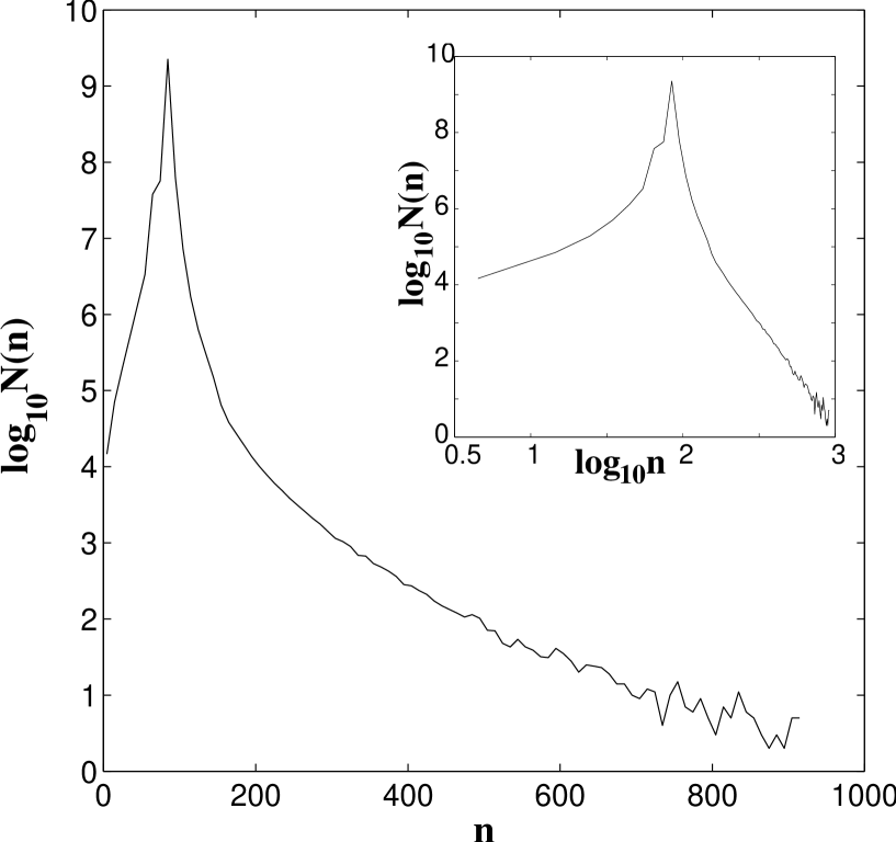
Figure 3: Distribution of the $\epsilon$-separation time intervals for $K=0.008$; $\epsilon_{0}=0.008$, obtained from 4048 reference trajectories and $10^{7}$ iterations each.

A typical distribution $N(n)$, where $n$ is discrete time and ${\bf A}$, ${\bf B}$ are omitted, is shown in Fig. 3 at the degeneracy point $K=\epsilon_{0}$. For the initial distance in pairs we select $d_{0}=10^{-6}$ and $\epsilon=10^{-2}$. All 4048 reference trajectories were run for $10^{7}$ iterations and full number of the separation events $N\sim 10^{9}$. There are 3 different regions in the behavior of $N(n)$. Before the sharp peak at $n_{p}\sim 100$ there is $N(n)\sim\exp(\bar{\sigma}n)$, where $\bar{\sigma}$ is of the order of the mean Lyapunov exponent (see more below). After the sharp peak, within the interval $\log_{10}n\in(2,2.2)$ there is an exponential decay of $N(n)$, and for $\log_{10}n>2.3$ the function $N(n)$ is close to the polynomial decay. The latter statement is provisional due to the lack of statistics and small time interval. Because of inhomogeneity of phase space, the finite time Lyapunov exponent $\sigma_{t}$ has a distribution function, and the first two domains with the peak fit the corresponding theory of the probabilistic analysis of the distribution of $\sigma_{t}$ (see for example in[15]). The third domain shows a new feature that can be interpreted as influence of the bifurcation point that leads to the appearance of the stickiness near $(x,y)=(0,0)$.

Another situation occurs for the values of parameters $(K^{*},\epsilon^{*})$, given in (12) when the stickiness to the hierarchical islands is strong. For this specific case, let us denote

$$P(n)=\lim_{N\rightarrow\infty}N(\tau,{\bf A},{\bf B})/N$$ (18)

(compare to (17)). A corresponding result is shown in Fig. 4. Within four decades of $n$ there is a clear power-wise behavior of $P(n)$:

$$P(n)\sim{\rm const.}\ n^{-\gamma}\ ,\ \ \ \ \ (n\rightarrow\infty)$$ (19)

with $\gamma\approx 3.3$. To analyze this result, we need to

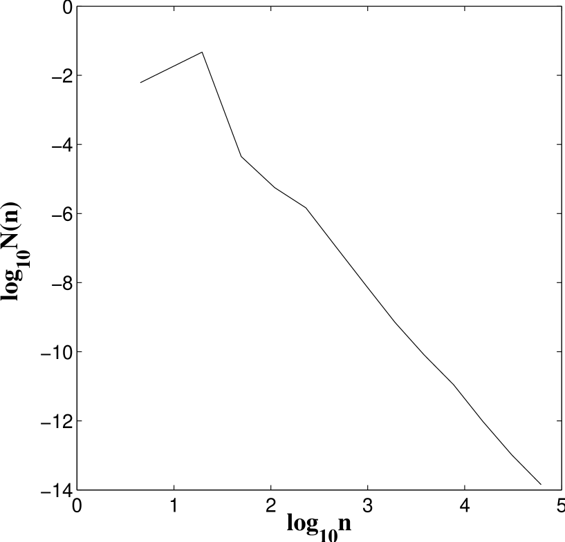
Figure 4: The same as in Fig. 3 but for special values $K^{*}=1$, $\epsilon_{0}^{*}=1.689538$.

Conjecture [9]: Assume that the phase space $\Gamma$ of compact dynamics can be split in two parts: ${\bf A}$ that corresponds to the only sticky (singular) zone and $\Gamma\backslash{\bf A}$, and that ${\bf A}\cap\Gamma\backslash{\bf A}=0$. Then for fairly small ${\bf B}\subset\Gamma\backslash{\bf A}$ the following equality is valid

$$\gamma_{\rm rec}=\gamma\ ,\ \ \ \ \ (t\rightarrow\infty)$$ (20)

where $\gamma_{\rm rec}$ is the recurrence exponent of the distribution of Poincaré recurrences to ${\bf B}$

$$P_{\rm rec}(n)={\rm const.}\ n^{-\gamma_{\rm rec}}$$

$$\sum_{n=1}^{\infty}P_{\rm rec}(n)=1\ .\ \ \ \ (n\rightarrow\infty)$$ (21)

In other words, distribution of $\epsilon$-dispersion of trajectories for small $\epsilon$ is defined asymptotically by the sticky zone.

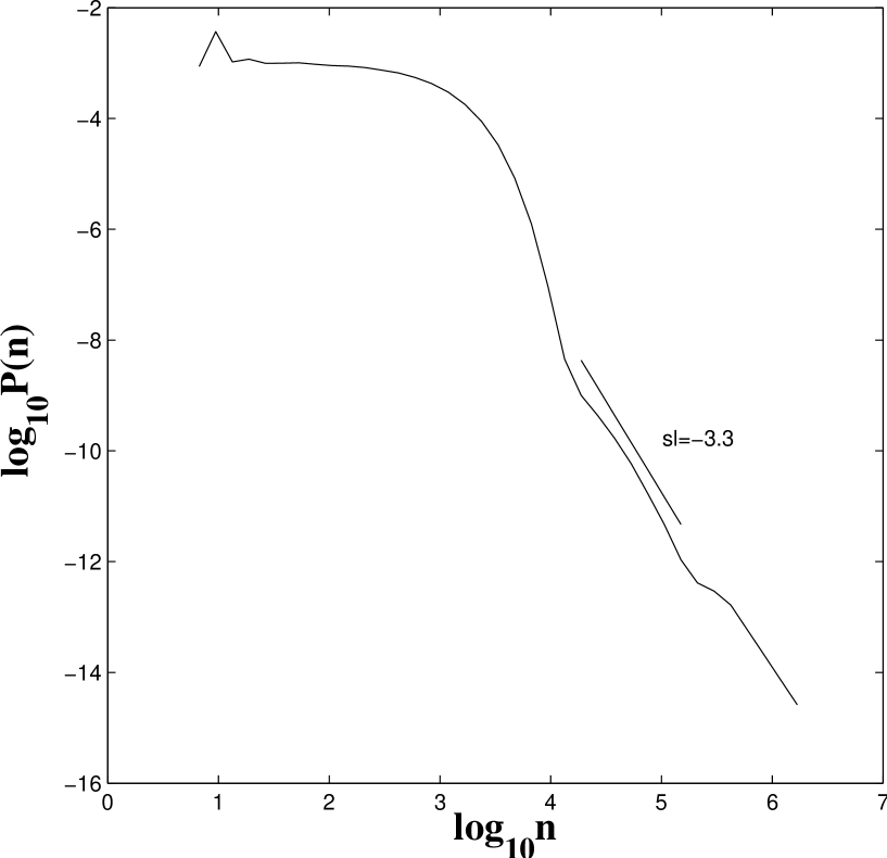
Figure 5: Distribution of Poincaré recurrence time for special values $K^{*}=1$, $\epsilon^{*}_{0}=1.689538$

The value $\gamma_{\rm rec}=3.3$ may be of a universal character since similar value was obtained for the standard map in [11]. It is worthwhile to check the statements (20) and (21) straightforward by calculating the distribution of Poincaré recurrences. The corresponding data are given in Fig. 5. For the time interval $n<10^{4}$

$$P_{\rm rec}(n)\sim\exp(-n/\bar{n})$$ (22)

but for $n>10^{4}$ there is a crossover to the power law (21) with the same exponent $\gamma_{\rm rec}=3.3$.

5. CONCLUSIONS

Our numerical results demonstrate that the perturbed Anosov map shows the features of the typical realistic Hamiltonian systems of low dimension: appearance of islands as a result of a bifurcation; sequence of topological changes in the phase space when we change parameters of the system; islands-around-islands hierarchical set; stickiness of the islands’ boundaries. The most important new features of the perturbed Anosov map is the transform of the Poincaré recurrences distribution from the exponential decay to the power-wise decay as $t\rightarrow\infty$. Such a change is important for numerous applications being responsible for different anomalous properties of the observable macroscopic characteristics [6].

Both, Property 1 and Property 2 formulated in Sec. 3, include as their main part the existence of different infinite hierarchies of islands. These statements are conjectures based on high accuracy simulations. The area of stickiness of orbits can be characterized by a low rate of dispersion of trajectories. That means that the long time, necessary for trajectories separation, can be effectively lower if the accuracy is insufficient. A possibility to observe a crossover from exponential dispersion of trajectories to the power one just confirms the high level of accuracy of simulations. To be more specific, let us mention that the critical value of perturbation $\epsilon_{0}^{*}$ is defined up to six decimal digits in (12). The crossover from the exponential decay of $P(n)$ to the power one occurs at $\log_{10}n\approx 4$ (see Fig. 5) and the power behavior of $P(n)$ is up to $\log_{10}n\geq 6$. These results are consistent with level of accuracy of $\epsilon_{0}^{*}$.

Acknowledgments

We are very grateful to L.M. Lerman for numerous discussions and a possibility to read his notes prior to publication. This work was supported by the Office of Naval Research Grant No. N00014-02-1-0056, and the U.S. Department of Energy Grant No. DE-FG02-92ER54184. Simulations were supported by NERSC.

REFERENCES

REFERENCES

- [1] J. Lewowicz, Lyapunov Functions and Topological Stability, J. Diff. Equations 38, 192-209 (1980).
- [2] F. Przytycki, Examples of conservative diffeomorphisms of the two-dimensional torus with co-existence of elliptic and stochastic behavior, Ergod. Th. & Dynam. Sys. 2, 439-463 (1982).
- [3] H. Enrich, A heteroclinic bifurcation of Anosov diffeomorphisms, Ergod. Th. & Dynam. Sys. 18, 567-608 (1998).
- [4] L.M. Lerman, not published (2004).
- [5] I. Dana and V.E. Chernov, Chaotic diffusion on periodic orbits: The perturbed Arnold cat map.
- [6] G.M. Zaslavsky, Chaos, fractional kinetics, and anomalous transport, Phys. Reports 371, 461-580 (2002).
- [7] V. Afraimovich and G.M. Zaslavsky, Space-time complexity in Hamiltonian systems, Chaos 13, 519-532 (2003).
- [8] X. Leoncini and G.M. Zaslavsky, Jets, stickiness, and anomalous transport, Phys. Rev. E 65, 046216-
- [9] G.M. Zaslavsky and M. Edelman, Polynomial dispersion of trajectories in sticky dynamics, Phys. Rev. E 72 (2005).
- [10] G.A. Margulis, Certain measures that are connected to -flows on compact manifolds, Funks. Anal. 1 Prilozh. 4, 62-76 (1970).
- [11] G.M. Zaslavsky, M. Edelman, and B.A. Niyazov, Self-similarity, renormalization, and phase space non-uniformity of Hamiltonian chaotic dynamics, Chaos 7, 159-181 (1997).
- [12] J.D. Hanson, J.R. Cary, J.D. Meiss, Algebraic decay in self-similar Markov chains, J. Stat. Phys. 39, 327-345 (1985).
- [13] G.M. Zaslavsky, Dynamical traps, Physica D 168-169, 292-304 (2002).
- [14] M. Kac, Probability and Related Topics in Physical Sciences, Interscience, New York, 1958.
- [15] E. Ott, Chaos in Dynamical Systems, Cambridge University Press, Cambridge, 1993.