Eddy diffusivity in convective hydromagnetic systems

Abstract

An eigenvalue equation, for linear instability modes involving large scales in a convective hydromagnetic system, is derived in the framework of multiscale analysis. We consider a horizontal layer with electrically conducting boundaries, kept at fixed temperatures and with free surface boundary conditions for the velocity field; periodicity in horizontal directions is assumed. The steady states must be stable to short (fast) scale perturbations and possess symmetry about the vertical axis, allowing instabilities involving large (slow) scales to develop. We expand the modes and their growth rates in power series in the scale separation parameter and obtain a hierarchy of equations, which are solved numerically. Second order solvability condition yields a closed equation for the leading terms of the asymptotic expansions and respective growth rate, whose origin is in the (combined) eddy diffusivity phenomenon. For about $10\%$ of randomly generated steady convective hydromagnetic regimes, negative eddy diffusivity is found.

1 Introduction

According to the present-day paradigm, magnetic fields of most astrophysical objects – the Earth and the outer planets of the Solar system having a molten metal fluid core (Merr, ), the Sun (Prie, ) and other stars, and even entire galaxies (RuSoShu, ) – owe their existence to convective hydromagnetic processes (Moff, ; Park, ; Zeld, ). Convection in the presence of a magnetic field obeys a familiar set of equations: the Navier-Stokes equation with Lorentz and Archimedes forces for the flow, the magnetic induction equation for the magnetic field, and the heat equation for temperature. Virtually no analytic solutions of this system of equations are known except for some significantly reduced cases (PoZa, ), under the assumption that certain symmetries are present, or for specific initial conditions. The referred set of equations may be used to simulate the evolution of astrophysical convective hydromagnetic systems. This approach was followed in (JoRo00, ; RoJo, ; JoRo, ), where magneto-convection in an idealised plane layer was considered, and in (GlRo95a, ; GlRo95b, ; GlRo96a, ; GlRo96b, ; GlRo97a, ; GlRo97b, ; RoGl, ; Jones, ), where the outer core of the Earth was modelled by three-dimensional equations of hydromagnetic convection in a spherical layer and, as a result, the predominant dipole morphology of the Earth’s magnetic field was correctly reproduced in computations.

However, in practice, accurate simulations for geo- and astrophysical real parameter values are close to impossible, because the limited power of available computers prohibits computations with the adequate spatial (insufficient memory) and temporal (insufficient CPU power) resolution. The simulations done by Glatzmaier and Roberts (GlRo95a, ; GlRo95b, ; GlRo96a, ; GlRo96b, ; GlRo97a, ; GlRo97b, ) were performed for parameter values differing by several orders of magnitude from those characterising the outer liquid core of the Earth. Nevertheless, the agreement between these simulations and the geodynamo is surprising (Jones, ). The existence of sharp contrast spatial structures (e.g., Ekman boundary layer, which emerges in convective flows in a rotating layer with no-slip boundary conditions, and the instability of which may be a source of dynamo (PoGiSo01a, ; PoGiSo01b, ; PoGiSo03, ; Rotv, ; Stell, )) and the prominent role which turbulence plays in the generation of magnetic fields, indicate that such a high resolution is indeed necessary in simulations. Core-mantle coupling, which is believed to cause decade variations of the length of day, is another geophysical phenomenon involving small scales (topographic features at the boundary are unlikely to exceed 5 km in amplitude; see (Merr, )). Validity of numerical techniques for smoothening the resolution cut-off, such as employment of hyperviscosity, is questionable (ZhaJo, ; Sars, ; ZhaSchu, ; Bus, ).

A significant uncertainty in rheology relations (ChrPel, ) and parameter values (PelPel, ) in the convective hydromagnetic equations (for instance, estimates of thermal diffusivity for the Earth core differ in several orders of magnitude (Merr, )), makes it desirable to investigate typical regimes of behaviour of the solutions by varying the parameters in certain ranges and finding locations, in the parameter space, of bifurcations marking drastic changes in behaviour (ChrOlGl, ). A purely numerical approach to the implementation of this task would require a further significant increase of the amount of computations. Consequently, a semi-analytic approach, employing asymptotic relations, is unavoidable as an alternative to both purely analytic and numerical approaches. Here we employ it to consider the problem of linear stability of three-dimensional convective hydromagnetic steady states in a layer.

The characteristic spatial scale of the perturbed steady state is supposed to be much larger than that of the steady state. The ratio of the spatial scale of the flow (fast spatial variable) to the large scale of perturbation (slow variable), $\varepsilon$, is a small parameter. (By small- and large-scale vector fields we refer to fields involving spatial scales of the order of the width of the layer and much larger scales, respectively.) Applying methods of the general theory of homogenisation of differential operators (Bens, ; Ole, ; Jik, ; Cio, ), we expand perturbation modes and their growth rates in asymptotic series in the parameter $\varepsilon$ and obtain a homogenised operator in slow variables, acting on mean fields. Eigenvalues of this operator control stability to large-scale perturbations. The advantage of this approach stems from opening the possibility to disentangle the large and small scales and fully resolve small scales by solving the so-called auxiliary problems.

Generically, the multiscale analysis reveals the presence of $\alpha$-effect (see (FrZhSu, ; SuShe, ; Zhe91, )). The homogenised linear operator is then the first-order differential operator. Consequently, the system is generically unstable, since the spectrum of the operator is symmetric about the origin (if a mode $\mathbf{W}(x)$ is associated with an eigenvalue $\lambda$, then $\mathbf{W}(-x)$ is a mode associated with the eigenvalue $-\lambda$). In convective hydromagnetic systems which possess symmetry about a vertical axis or parity-invariance, $\alpha$-effect is not present and the homogenised equations involve a second-order partial differential operator, whose eigenfunctions are Fourier harmonics. Its eigenvalues may be positive, implying instability. This phenomenon is referred to as negative (combined) eddy diffusivity (Star, ). Instability of this kind is weak: in the presence of $\alpha$-effect the growth rate of the dominant perturbations is $O(\varepsilon)$, whereas it is $O(\varepsilon^{2})$ when $\alpha$-effect is absent. Evaluation of eddy tensors emerging in the homogenised equations requires solution of auxiliary problems, which are linear elliptic partial differential equations in fast variables. With just a single characteristic spatial scale involved, they are not too demanding numerically.

Multiscale asymptotic analysis was successfully applied to various problems of hydrodynamics and magnetohydrodynamics. The effect of negative eddy viscosity arises in two-dimensional (SiYa, ; SiFre, ; GaVeFr, ) and three-dimensional (Yu90, ; DubFr, ; WiGaFr, ) hydrodynamic systems, if the flow is parity-invariant or if it is a Beltrami field (in (Yu90, ) large scale along only one direction was assumed). Eddy diffusivity can be complex (Wirth, ; WiGaFr, ). In generic hydrodynamic systems, which do not possess the properties mentioned above, similar expansions indicate the presence of the so-called AKA-effect (i.e. anisotropic kinetic $\alpha$-effect) (FrZhSu, ; SuShe, ). In passive scalar transport systems, eddy diffusivity can only enhance molecular diffusivity (Bife, ; VeAv, ).

In the kinematic dynamo problem (concerning magnetic field generation, when the feedback influence of magnetic field on the flow via the Lorentz force is neglected), multiscale expansions were apparently first introduced in (Chi, ) and (Sow, ) (where scale separation was related to fast rotation of the layer of conducting fluid). Similar asymptotic expansions in the kinematic problem (for flows, the amplitude of which may depend on the scale ratio) predict occurrence of $\alpha$-effect (Vi86, ; Vi87, ; Zhe91, ). Generation of large-scale magnetic field by the negative magnetic eddy diffusivity mechanism is possible for parity-invariant steady (Lano, ; Zhe01, ; Yu01, ) (in (Yu01, ), large scale along only one direction was assumed) or time-periodic flows (ZhePo, ), and by convective Bisshopp cell patterns (Zhe05, ), symmetric about the vertical axis. Combined eddy diffusivity tensors for large-scale perturbations of both the flow and magnetic field constituting a parity-invariant three-dimensional MHD steady state were derived in (Zhe03, ).

In the papers cited above two different scales were present in the system. Multiscale expansions with three spatial scales were employed in (Po05, ; Po05mjg, ) to study the small-angle instability (Cox, ) in convection in a rotating layer.

Evolution of a mean hydrodynamic large-scale perturbation in the weakly nonlinear regime was considered in the absence of magnetic field for two-dimensional parity-invariant space-periodic flows (GaVeFr, ; PoPaSu, ), and for three-dimensional MHD systems (Zhe05fz, ). In (Zhe05fz, ) it is not required that the MHD state, nonlinear stability of which is examined, is either space periodic or steady; equations for the mean flow and magnetic field are generalisations of the Navier-Stokes and magnetic induction equation with an anisotropic (in general) combined eddy diffusivity tensor and quadratic eddy advection.

In section 2, we present the equations for thermal convection in the presence of magnetic field and discuss boundary conditions and symmetries. In section 3, the multiscale formalism is applied. In section 3.1, an eigenfunction of the linearisation of a convective hydromagnetic system and its associated eigenvalue are expanded in a power series of the scale separation parameter and a hierarchy of equations is derived. In section 3.2, the solvability condition, which plays an important role in solution of equations of this hierarchy and in derivation of an equation for the mean part of perturbation in the leading order, is discussed. In sections 3.3 and 3.4, the first two (order 0 and order 1) equations in the hierarchy are expressed as a linear combination of the so-called auxiliary problems. In section 3.5, we consider the solvability condition for equations at order 2 and thereby derive the eigenvalue equation for the mean part of the leading terms in the expansions of the instability modes and their growth rates. At this stage emerges the homogenised combined eddy diffusivity operator acting on mean fields. In section 4, we briefly describe the numerical procedure for solving the auxiliary problems and present a set of basic fields which lead to large-scale instability for appropriate physical parameters (namely molecular diffusivities). Finally (section 5), we comment on possible extensions and limitations of the application of multiscale techniques employed here to study the instability of convective flows in the presence of magnetic field.

2 Equations of thermal convection in the presence of magnetic field

2.1 Time evolution of a convective hydromagnetic system

Magnetic field generation by thermal convection is governed by the Navier-Stokes equation, the magnetic induction equation and heat transfer equation (Chan, ):

$$\partial_{t}\mathbf{V} = \mathbf{V}\times(\partial\times\mathbf{V})-\partial p+\nu\partial^{2}\mathbf{V}$$

$$-\mathbf{H}\times(\partial\times\mathbf{H})-\alpha(T-T_{0})\mathbf{G}+\tilde{\mathbf{F}},$$

$$\partial\cdot\mathbf{V} = 0,$$

$$\partial_{t}\mathbf{H} = \partial\times(\mathbf{V}\times\mathbf{H})+\eta\partial^{2}\mathbf{H}+\tilde{\mathbf{R}},$$ (1)

$$\partial\cdot\mathbf{H} = 0,$$

$$\partial_{t}\,T = -(\mathbf{V}\cdot\partial)T+k\partial^{2}T+\frac{\sigma}{2}\left|\partial\times\mathbf{H}\right|^{2}+\tilde{S},$$

where $\mathbf{V}=(V_{1},V_{2},V_{3})$, $\mathbf{H}=(H_{1},H_{2},H_{3})$ and $T$, depending on position in space $\mathbf{x}=(x_{1},x_{2},x_{3})$ and time $t$, are the velocity field, the magnetic field and the temperature, respectively. We use the notation $\partial_{t}\equiv\partial/\partial t$, $\partial_{i}\equiv\partial/\partial x_{i}$ and $\partial\equiv\sum_{i=1}^{3}\mathbf{e}_{i}\partial_{i}$, where $\mathbf{e}_{i}$ is the ith canonical vector. The term involving $\mathbf{G}$ (gravity, $\mathbf{G}=-g\,\mathbf{e}_{3}$ for a horizontal layer) is the buoyancy force due to temperature variation and $\mathbf{H}\times(\partial\times\mathbf{H})$ is the Lorentz force. $\tilde{\mathbf{F}}$ represents any other body forces acting on the fluid, $\tilde{\mathbf{R}}$ is due to imposed external currents or magnetic fields, and $\tilde{S}$ describes the distribution of external heat sources. $\nu$ is the kinematic viscosity, $\eta$ the magnetic diffusivity, and $\alpha$, $k$ and $\sigma$ are parameters related to thermal expansion, thermal conductivity and electrical conductivity, respectively. Solenoidality of magnetic field follows from the Maxwell equations. Flows are deemed incompressible in line with the Boussinesq approximation. Henceforth, the system of equations (1) will be referred to as CHM (convective hydromagnetic).

We consider the CHM equations in the spatial domain ${\cal D}=[0,L_{1}]\times[0,L_{2}]\times[0,L_{3}]$, assuming periodicity in $x_{1}$ and $x_{2}$ directions, and considering a finite layer in the $x_{3}$ direction. The boundary conditions at the surface of the layer are

$\bullet$ for the velocity field:

$$V_{3}|_{x_{3}=0,L_{3}}=0,$$

$$\partial_{3}V_{1}|_{x_{3}=0,L_{3}}=\partial_{3}V_{2}|_{x_{3}=0,L_{3}}=0;$$

$\bullet$ for the magnetic field:

$$H_{3}|_{x_{3}=0,L_{3}}=0,$$

$$\partial_{3}H_{1}|_{x_{3}=0,L_{3}}=\partial_{3}H_{2}|_{x_{3}=0,L_{3}}=0;$$

$\bullet$ for the temperature field:

$$T|_{x_{3}=0}=T_{1},$$

$$T|_{x_{3}=L_{3}}=T_{2}.$$

It is convenient to introduce the variable

$$\theta=T-T_{1}-\delta Tx_{3},$$

where $\delta T=(T_{2}-T_{1})/L_{3}$, satisfying the uniform boundary conditions

$$\theta|_{x_{3}=0,L_{3}}=0.$$

A solution to the CHM system may possess symmetry about the vertical axis, provided the forcing terms $\tilde{\mathbf{F}},\tilde{\mathbf{R}},\tilde{S}$ possess the same symmetry. A vector field $\mathbf{Q}$ is called symmetric (about the vertical axis) if

$$Q_{1}(-x_{1},-x_{2},x_{3})=-Q_{1}(x_{1},x_{2},x_{3}),$$

$$Q_{2}(-x_{1},-x_{2},x_{3})=-Q_{2}(x_{1},x_{2},x_{3}),$$

$$Q_{3}(-x_{1},-x_{2},x_{3})=Q_{3}(x_{1},x_{2},x_{3});$$

and anti-symmetric if

$$Q_{1}(-x_{1},-x_{2},x_{3})=Q_{1}(x_{1},x_{2},x_{3}),$$

$$Q_{2}(-x_{1},-x_{2},x_{3})=Q_{2}(x_{1},x_{2},x_{3}),$$

$$Q_{3}(-x_{1},-x_{2},x_{3})=-Q_{3}(x_{1},x_{2},x_{3}).$$

We call a scalar field $f$ symmetric if

$$f(-x_{1},-x_{2},x_{3})=f(x_{1},x_{2},x_{3}),$$

and anti-symmetric if

$$f(-x_{1},-x_{2},x_{3})=-f(x_{1},x_{2},x_{3}).$$

Symmetries are essential to eliminate first order (alpha) effects. In (DubFr, ) parity-invariance is used to this purpose, but, for a horizontal layer, symmetry about the vertical axis is more realistic. Furthermore, parity invariance is inconsistent with the basic equations (1) for $\sigma\neq 0.$ Under an appropriate forcing, any hydromagnetic convective system will possess steady states with these symmetries.

2.2 Linearised CHM operator

Let us consider a steady state solution, $\tilde{p}$, $\tilde{\mathbf{V}}$, $\tilde{\mathbf{H}}$ and $\tilde{\theta}$, of the CHM system (1) and a small perturbation, $pe^{\lambda t}$, $\mathbf{V}e^{\lambda t}$, $\mathbf{H}e^{\lambda t}$ and $\theta e^{\lambda t}$, of this steady state, where $p$, $\mathbf{V}$, $\mathbf{H}$ and $\theta$ depend only on spatial variables. In what follows, we will call the spatial profiles of the perturbation fields, $p$, $\mathbf{V}$, $\mathbf{H}$ and $\theta$, a perturbation. Replacing $p$, $\mathbf{V}$, $\mathbf{H}$, $\theta$, respectively, by $\tilde{p}+pe^{\lambda t}$, $\tilde{\mathbf{V}}+\mathbf{V}e^{\lambda t}$, $\tilde{\mathbf{H}}+\mathbf{H}e^{\lambda t}$, $\tilde{\theta}+\theta e^{\lambda t}$ in (1) and neglecting second order terms in the perturbation, we obtain an eigenvalue problem for the perturbation:

$$\begin{array}[]{l}\mathbf{A}\mathbf{W}=\lambda\mathbf{W}+\left[\begin{array}[]{c}\partial p\\ \mathbf{0}\\ 0\end{array}\right],\\ \partial\cdot\mathbf{V}=0,\\ \partial\cdot\mathbf{H}=0.\end{array}$$ (2)

Here, the block notation introduced in (DubFr, ) is used:

$$\mathbf{W}=\left[\begin{array}[]{c}\mathbf{V}\\ \mathbf{H}\\ \theta\end{array}\right],$$ (3)

is the $(3+3+1)$-dimensional block column vector combining the 3 components of the flow, the 3 components of the magnetic field and the temperature field. In what follows, $(3+3+1)$-dimensional vectors of a similar structure, will be used. The operator $\mathbf{A}$ is obtained by linearisation of the CHM equations in the vicinity of the steady state $\tilde{p}$, $\tilde{\mathbf{V}}$, $\tilde{\mathbf{H}}$ and $\tilde{\theta}$; it can be represented as a block matrix (acting on $(3+3+1)$-dimensional vectors of the structure similar to (3)):

$$\mathbf{A} = \left[\begin{array}[]{lllll}\nu\partial^{2}+\tilde{\mathbf{V}}\times(\partial\times\bullet)-(\partial\times\tilde{\mathbf{V}})\times&&-\tilde{\mathbf{H}}\times(\partial\times\bullet)+(\partial\times\tilde{\mathbf{H}})\times&&-\alpha\,\mathbf{G}\\ -\partial\times(\tilde{\mathbf{H}}\times\bullet)&&\eta\partial^{2}+\partial\times(\tilde{\mathbf{V}}\times\bullet)&&\mathbf{0}\\ -(\bullet\cdot\partial)\tilde{\theta}-\delta T\mathbf{e}_{3}\cdot&&\sigma(\partial\times\tilde{\mathbf{H}})\cdot(\partial\times\bullet)&&k\,\partial^{2}-\tilde{\mathbf{V}}\cdot\partial\end{array}\right].$$ (7)

Note that $\mathbf{A}$ preserves the symmetry of fields $\mathbf{W}$, symmetric (or anti-symmetric) about the vertical axis.

The complete formulation of the eigenvalue problem (2) involves specifying spatial periods of perturbations, which can be any integer multiples of the periods $L_{1}$ and $L_{2}$. If the smallest of the periodicity boxes is considered, the system of equations (2) is referred to as the problem of linear stability to short-scale perturbations.

3 Linearised large-scale CHM equation

3.1 The two-scales expansion

In this section we construct a homogenisation of the linearised CHM operator. Eigenvalues of the homogenised operator control linear stability of the CHM steady state to perturbations with spatial periods large enough for the asymptotic behaviour to set in.

Following the method applied in previous studies (Lano, ; Zhe01, ; Zhe03, ; ZhePo, ), we consider fast variables, $\mathbf{x}$, representing the short scale dynamics, and slow variables, $\mathbf{X}=(X_{1},X_{2})=(\varepsilon x_{1},\varepsilon x_{2})$, representing the large scale dynamics. (In a layer of finite width only slow variables in horizontal directions are geometrically consistent.) The parameter $\varepsilon$ is the scale separation. The perturbations $p$, $\mathbf{V}$, $\mathbf{H}$ and $\theta$ are assumed to depend on both fast and slow variables. We denote $\nabla_{i}\equiv\partial/\partial X_{i}$ and $\nabla\equiv\sum_{i=1}^{2}\mathbf{e}_{i}\nabla_{i}$.

Now we perform differentiation in (2) applying the chain rule: $\partial_{i}\rightarrow\partial_{i}+\varepsilon\nabla_{i}$ for $i=1,2$. This implies

$$\mathbf{A}=\mathbf{A}^{(0)}+\varepsilon\mathbf{A}^{(1)}+\varepsilon^{2}\mathbf{A}^{(2)},$$

where

$$\mathbf{A}^{(0)} = \left[\begin{array}[]{lclll}\nu\partial^{2}+\tilde{\mathbf{V}}\times(\partial\times\bullet)-(\partial\times\tilde{\mathbf{V}})\times&&-\tilde{\mathbf{H}}\times(\partial\times\bullet)+(\partial\times\tilde{\mathbf{H}})\times&&-\alpha\,\mathbf{G}\\ -\partial\times(\tilde{\mathbf{H}}\times\bullet)&&\eta\partial^{2}+\partial\times(\tilde{\mathbf{V}}\times\bullet)&&\mathbf{0}\\ -(\bullet\cdot\partial)\tilde{\theta}-\delta T\mathbf{e}_{3}\cdot&&\sigma(\partial\times\tilde{\mathbf{H}})\cdot(\partial\times\bullet)&&k\,\partial^{2}-\tilde{\mathbf{V}}\cdot\partial\end{array}\right],$$ (11)

$$\mathbf{A}^{(1)} = \left[\begin{array}[]{lclcl}2\nu\partial\cdot\nabla+\tilde{\mathbf{V}}\times(\nabla\times\bullet)&&-\tilde{\mathbf{H}}\times(\nabla\times\bullet)&&\mathbf{0}\\ -\nabla\times(\tilde{\mathbf{H}}\times\bullet)&&2\eta\partial\cdot\nabla+\nabla\times(\tilde{\mathbf{V}}\times\bullet)&&\mathbf{0}\\ 0&&\sigma(\partial\times\tilde{\mathbf{H}})\cdot(\nabla\times\bullet)&&2k\partial\cdot\nabla-\tilde{\mathbf{V}}\cdot\nabla\end{array}\right],$$ (15)

$$\mathbf{A}^{(2)} = {\mathbf{\Xi}}\nabla^{2},\textrm{ with }\ {\mathbf{\Xi}}=\left[\begin{array}[]{ccc}\nu&\mathbf{0}&\mathbf{0}\\ \mathbf{0}&\eta&\mathbf{0}\\ 0&0&k\end{array}\right]$$ (19)

(${\mathbf{\Xi}}$ is the molecular diffusivity tensor). Note that $\mathbf{A}^{(0)}$ and $\mathbf{A}^{(2)}$ preserve the symmetries of both symmetric and anti-symmetric fields, but $\mathbf{A}^{(1)}$ exchanges their symmetry.

Next we expand $\mathbf{W}$, $p$ and $\lambda$ in power series of $\varepsilon$:

$$\mathbf{W}=\sum_{i=0}^{n}\varepsilon^{i}\mathbf{W}^{(i)}+O(\varepsilon^{n+1}),$$ (20)

$$p=\sum_{i=0}^{n}\varepsilon^{i}p^{(i)}+O(\varepsilon^{n+1}),$$ (21)

$$\lambda=\sum_{i=0}^{n}\varepsilon^{i}\lambda_{i}+O(\varepsilon^{n+1}).$$ (22)

Each coefficient $\mathbf{W}^{(i)}$ and $p^{(i)}$ in the expansions is a function of both $\mathbf{x}$ and $\mathbf{X}$. Substituting these series in (2) and equating the terms in $\varepsilon^{n}$, at each order $n$, we obtain a hierarchy of equations:

• order 0:

  $$\mathbf{A}^{(0)}\mathbf{W}^{(0)} = \lambda_{0}\mathbf{W}^{(0)}+\left[\begin{array}[]{c}\partial p^{(0)}\\ \mathbf{0}\\ 0\end{array}\right],$$ (26)

  $$\partial\cdot\mathbf{V}^{(0)} = 0,$$ (27)

  $$\partial\cdot\mathbf{B}^{(0)} = 0,$$ (28)

• order 1:

  $$\mathbf{A}^{(0)}\mathbf{W}^{(1)} = -\mathbf{A}^{(1)}\mathbf{W}^{(0)}+\lambda_{0}\mathbf{W}^{(1)}+\lambda_{1}\mathbf{W}^{(0)}+\left[\begin{array}[]{c}\partial p^{(1)}+\nabla p^{(0)}\\ \mathbf{0}\\ 0\end{array}\right],$$ (32)

  $$\partial\cdot\mathbf{V}^{(1)} = -\nabla\cdot\mathbf{V}^{(0)},$$ (33)

  $$\partial\cdot\mathbf{B}^{(1)} = -\nabla\cdot\mathbf{B}^{(0)},$$ (34)

• order 2:

  $$\mathbf{A}^{(0)}\mathbf{W}^{(2)} = -\mathbf{A}^{(1)}\mathbf{W}^{(1)}-\mathbf{A}^{(2)}\mathbf{W}^{(0)}+\lambda_{0}\mathbf{W}^{(2)}+\lambda_{1}\mathbf{W}^{(1)}+\lambda_{2}\mathbf{W}^{(0)}+\left[\begin{array}[]{c}\partial p^{(2)}+\nabla p^{(1)}\\ \mathbf{0}\\ 0\end{array}\right],$$ (38)

  $$\partial\cdot\mathbf{V}^{(2)} = -\nabla\cdot\mathbf{V}^{(1)},$$ (39)

  $$\partial\cdot\mathbf{B}^{(2)} = -\nabla\cdot\mathbf{B}^{(1)},$$ (40)

• order $n$:

  $$\mathbf{A}^{(0)}\mathbf{W}^{(n)} = -\mathbf{A}^{(1)}\mathbf{W}^{(n-1)}-\mathbf{A}^{(2)}\mathbf{W}^{(n-2)}+\sum_{i=0}^{n}\lambda_{i}\mathbf{W}^{(n-i)}+\left[\begin{array}[]{c}\partial p^{(n)}+\nabla p^{(n-1)}\\ \mathbf{0}\\ 0\end{array}\right],$$ (44)

  $$\partial\cdot\mathbf{V}^{(n)} = -\nabla\cdot\mathbf{V}^{(n-1)},$$ (45)

  $$\partial\cdot\mathbf{B}^{(n)} = -\nabla\cdot\mathbf{B}^{(n-1)}.$$ (46)

Let $\langle\bullet\rangle=(L_{1}L_{2}L_{3})^{-1}\int_{{\cal D}}\bullet dx_{1}dx_{2}dx_{3}$ denote the mean (over the fast variables in ${\cal D}$) and $\{\bullet\}=\bullet-\langle\bullet\rangle$ denote the fluctuating part of a vector or scalar field here denoted indistinguishably by $\bullet$. The average $\langle\bullet\rangle$ is the large scale component of the respective field. It is possible to solve recursively all equations in the hierarchy, finding all terms of the expansions (20)-(22). Only the equations up to order 2 are required to derive a homogenised eigenvalue equation for the mean parts, $\langle\mathbf{W}^{(0)}\rangle$ and $\langle p^{(0)}\rangle$, of the leading terms. It emerges as the solvability condition for the equation in the fast variables at order 2.

3.2 Solvability Conditions

Let $\mathbf{P}$ be the projection into the subspace of $(3+3+1)$-dimensional fields, in which the 3-dimensional vector components are solenoidal:

$$\mathbf{P}\left[\begin{array}[]{l}\mathbf{Q}^{\mathbf{V}}\\ \mathbf{Q}^{\mathbf{H}}\\ Q^{\theta}\end{array}\right]=\left[\begin{array}[]{l}\mathbf{Q}^{\mathbf{V}}-\partial Q^{\mathbf{V}p}\\ \mathbf{Q}^{\mathbf{H}}-\partial Q^{\mathbf{H}p}\\ Q^{\theta}\end{array}\right],$$

where $\partial^{2}Q^{\mathbf{V}p}=\partial\cdot\mathbf{Q}^{V}$ and $\partial^{2}Q^{\mathbf{H}p}=\partial\cdot\mathbf{Q}^{H}$. In what follows, we will solve equations of the form

$$\mathbf{P}\mathbf{A}^{(0)}\mathbf{f}=Pg,$$

where vector components of $\mathbf{f}$ are required to be solenoidal; this equation is thus equivalent to

$$\mathbf{P}\mathbf{A}^{(0)}\mathbf{P}f=\mathbf{P}g.$$ (47)

By the Fredholm alternative (Rie90, ), a solution of (47) exists if and only if $\mathbf{P}g$ is orthogonal to the kernel of $(\mathbf{P}\mathbf{A}^{(0)}\mathbf{P})^{*}$, where $*$ denotes the adjoint operator. In other words, the solvability condition for (47) is $\langle\mathbf{P}g,c\rangle=0$, where $\mathbf{c}$ is any vector in $\textrm{ker}(\mathbf{P}\mathbf{A}^{(0)^{*}}\mathbf{P})$ and $\langle\cdot,\cdot\rangle$ denotes the ${\cal L}^{2}$ inner product. As usual, the adjoint operator $\mathbf{A}^{(0)^{*}}$ can be derived performing integration by parts in the identity $\langle\mathbf{A}^{(0)^{*}}\mathbf{W}_{1},\mathbf{W}_{2}\rangle=\langle\mathbf{W}_{1},\mathbf{A}^{(0)}\mathbf{W}_{2}\rangle$. In the present case

$$\mathbf{A}^{(0)^{*}}=\left[\begin{array}[]{lllll}\nu\partial^{2}-\partial\,\times(\tilde{\mathbf{V}}\times\bullet)+(\partial\times\tilde{\mathbf{V}})\times&&\tilde{\mathbf{H}}\times(\partial\times\bullet)&&-\mathbf{e}_{3}\delta T+\tilde{\theta}\partial\\ \partial\times(\tilde{\mathbf{H}}\times\bullet)-(\partial\times\tilde{\mathbf{H}})\times&&\eta\partial^{2}-\tilde{\mathbf{V}}\times(\partial\times\bullet)&&\sigma\partial\times(\partial\times\tilde{\mathbf{H}})-\sigma(\partial\times\tilde{\mathbf{H}})\times(\partial\bullet)\\ -\alpha\mathbf{G}\,\cdot&&0&&k\partial^{2}+\tilde{\mathbf{V}}\cdot\partial\end{array}\right].$$

Boundary conditions for the vector fields in the domain of $\mathbf{A}^{(0)^{*}}$ can be found from the condition that boundary surface integrals, emerging in integration by parts in the scalar product $\langle\mathbf{W}_{1},\mathbf{A}^{(0)}\mathbf{W}_{2}\rangle$, vanish. It can be verified that the boundary conditions that we assume hold for vector fields in the domain of the adjoint operator as well.

Our construction relies on the existence of vector fields in $\textrm{ker}(\mathbf{P}\mathbf{A}^{(0)}\mathbf{P})$ with non-vanishing average horizontal components of the flow and magnetic field (see a detailed discussion in (Zhe05, )). It can be easily established that the dimension of the subspace of $\textrm{ker}(\mathbf{P}\mathbf{A}^{(0)}\mathbf{P})$, consisting of such vectors, is equal to the dimension of the subspace of $\textrm{ker}(\mathbf{P}\mathbf{A}^{(0)^{*}}\mathbf{P})$ consisting of vectors with non-zero horizontal space averages. If $\mathbf{c}=\left[\begin{array}[]{c}\mathbf{c}^{V}\\ \mathbf{c}^{H}\\ 0\end{array}\right]$, where $\mathbf{c}^{V}$ and $\mathbf{c}^{H}$ are any constant horizontal vectors, evidently $\mathbf{P}\mathbf{A}^{(0)^{*}}\mathbf{P}c=0$, since $\mathbf{A}^{(0)^{*}}\mathbf{c}$ is a gradient. Such constant vector fields satisfy the boundary conditions under consideration; therefore any such $\mathbf{c}$ belongs to $\textrm{ker}(\mathbf{P}\mathbf{A}^{(0)^{*}}\mathbf{P})$. Thus, $\textrm{ker}(\mathbf{P}\mathbf{A}^{(0)}\mathbf{P})$ is at least four-dimensional. In what follows, we assume that the dimension is four, which is generically the case, and thus any non-zero vector from $\textrm{ker}(\mathbf{P}\mathbf{A}^{(0)}\mathbf{P})$ has non-zero horizontal averages of the flow and/or magnetic field components. Then the solvability condition for (47) consists of orthogonality of $\mathbf{g}^{V}$ and $\mathbf{g}^{H}$ to constant horizontal vectors, i.e. the horizontal components of $\langle\mathbf{g}^{V}\rangle$ and $\langle\mathbf{g}^{H}\rangle$ must vanish.

3.3 Equations at order 0

Decoupling of the large- and short-scale behaviour is evident in the form of solutions of the equations emerging at orders 0 and 1 in the hierarchy. Since $\mathbf{A}^{(0)}$ is an operator in the fast variables, short-scale variation of these solutions is exclusively due to their multiplicative dependence on solutions of (26)-(28) and (32)-(34) – the so-called auxiliary problems, which are partial differential equations in the fast variables.

Performing integration and using the boundary conditions, we find that the horizontal components of the flow and magnetic field components of $\langle\mathbf{A}^{(0)}\mathbf{W}^{(0)}\rangle$ vanish. Since we seek solutions where $\langle\mathbf{V}^{(0)}\rangle$ and $\langle\mathbf{H}^{(0)}\rangle$ do not vanish simultaneously, averaging of (26) implies $\lambda_{0}=0$. The problem to solve becomes

$$\mathbf{A}^{(0)}\mathbf{W}^{(0)}=\left[\begin{array}[]{c}\partial p^{(0)}\\ \mathbf{0}\\ 0\end{array}\right].$$ (48)

By linearity,

$$\mathbf{W}^{(0)}=\sum_{i=1}^{4}a_{i}\,\mathbf{S}_{i},\quad\{p^{(0)}\}=\sum_{i=1}^{4}a_{i}\,S_{i}^{p}.$$ (49)

The fields $\mathbf{S}_{i}=\left[\begin{array}[]{c}\mathbf{S}_{i}^{\mathbf{V}}\\ \mathbf{S}_{i}^{\mathbf{H}}\\ S_{i}^{\theta}\end{array}\right]$ and $S_{i}^{p}$ are linearly independent solutions of the problems

$$\begin{array}[]{l}\mathbf{A}^{(0)}\mathbf{S}_{i}=\left[\begin{array}[]{c}\partial S_{i}^{p}\\ \mathbf{0}\\ 0\end{array}\right],\\ \partial\cdot\mathbf{S}_{i}^{\mathbf{V}}=0,\\ \partial\cdot\mathbf{S}_{i}^{\mathbf{H}}=0,\end{array}$$ (50)

i.e. $\mathbf{S}_{i}$ are linearly independent fields in $\textrm{ker}(\mathbf{P}\mathbf{A}^{(0)}\mathbf{P})$. The gradient part of (50) satisfies

$$\partial^{2}S_{i}^{p}=\partial\cdot\left(\mathbf{A}^{(0)}\mathbf{S}_{i}\right)^{\mathbf{V}}.$$ (51)

Note that $\langle p^{(0)}\rangle$ cannot be determined at this order, since derivatives in the fast variables in the r.h.s. of (48) eliminate any averages in $p^{(0)}$. $\mathbf{S}_{i}$ and $S_{i}^{p}$ depend only on the fast variables. The coefficients of the linear combinations ((49)), $a_{i}$, depend only on the slow variables.

The four possible averages (constant mean fields) in $\textrm{ker}(\mathbf{P}\mathbf{A}^{(0)}\mathbf{P})$, selected by the boundary conditions, are

$$\begin{array}[]{cc}\langle\mathbf{S}_{1}\rangle=\left[\begin{array}[]{c}\mathbf{e}_{1}\\ \mathbf{0}\\ 0\end{array}\right],&\langle\mathbf{S}_{2}\rangle=\left[\begin{array}[]{c}\mathbf{e}_{2}\\ \mathbf{0}\\ 0\end{array}\right],\end{array}$$

$$\begin{array}[]{cc}\langle\mathbf{S}_{3}\rangle=\left[\begin{array}[]{c}\mathbf{0}\\ \mathbf{e}_{1}\\ 0\end{array}\right],&\langle\mathbf{S}_{4}\rangle=\left[\begin{array}[]{c}\mathbf{0}\\ \mathbf{e}_{2}\\ 0\end{array}\right]\end{array}.$$

Hence, the four auxiliary problems at order 0 are

$$\mathbf{A}^{(0)}\{\mathbf{S}_{1}\}=\left[\begin{array}[]{c}\partial(S_{1}^{p}-\tilde{\mathbf{V}}_{1})+\partial_{1}\tilde{\mathbf{V}}\\ \partial_{1}\tilde{\mathbf{H}}\\ \partial_{1}\tilde{\theta}\end{array}\right],$$ (52)

$$\mathbf{A}^{(0)}\{\mathbf{S}_{2}\}=\left[\begin{array}[]{c}\partial(S_{2}^{p}-\tilde{\mathbf{V}}_{2})+\partial_{2}\tilde{\mathbf{V}}\\ \partial_{2}\tilde{\mathbf{H}}\\ \partial_{2}\tilde{\theta}\end{array}\right],$$ (53)

$$\mathbf{A}^{(0)}\{\mathbf{S}_{3}\}=\left[\begin{array}[]{c}\partial(S_{3}^{p}+\tilde{\mathbf{H}}_{1})-\partial_{1}\tilde{\mathbf{H}}\\ -\partial_{1}\tilde{\mathbf{V}}\\ 0\end{array}\right],$$ (54)

$$\mathbf{A}^{(0)}\{\mathbf{S}_{4}\}=\left[\begin{array}[]{c}\partial(S_{4}^{p}+\tilde{\mathbf{H}}_{2})-\partial_{2}\tilde{\mathbf{H}}\\ -\partial_{2}\tilde{\mathbf{V}}\\ 0\end{array}\right],$$ (55)

with $S_{i}^{p}$ given by (51).

Solenoidal parts of the right hand sides of (52)-(55) are anti-symmetric and, since $\mathbf{A}^{(0)}$ preserves the symmetry of fields, $\mathbf{S}_{i}$ are anti-symmetric. Evidently, the order 0 auxiliary problems are of the form of (47), and their solvability follows immediately from the periodicity of the CHM steady state $\tilde{\mathbf{V}}$, $\tilde{\mathbf{H}}$, $\tilde{\theta}$ in horizontal directions.

3.4 Equations at order 1

Averaging of (32) yields

$$\left\langle\mathbf{A}^{(0)}\mathbf{W}^{(1)}\right\rangle=-\left\langle\mathbf{A}^{(1)}\mathbf{W}^{(0)}\right\rangle+\lambda_{1}\langle\mathbf{W}^{(0)}\rangle+\left[\begin{array}[]{c}\nabla\langle p^{(0)}\rangle\\ \mathbf{0}\\ 0\end{array}\right].$$ (56)

As in order 0, horizontal parts of the flow and magnetic field components of $\langle\mathbf{A}^{(0)}\mathbf{W}^{(1)}\rangle$ are zero. The same holds for $\langle\mathbf{A}^{(1)}\mathbf{W}^{(0)}\rangle$ (this can be shown, integrating directly the terms of the form of spatial derivatives and using the boundary conditions, and exploiting the symmetry of the perturbed CHM steady state and anti-symmetry in the fast variables of $\mathbf{V}^{(0)}$ and $\mathbf{H}^{(0)}$ when considering mean horizontal parts of the terms of the form of $\tilde{\mathbf{V}}\times(\nabla\times\mathbf{V}^{(0)})$). (56) becomes

$$\lambda_{1}\langle\mathbf{W}^{(0)}\rangle+\left[\begin{array}[]{c}\nabla\langle p^{(0)}\rangle\\ \mathbf{0}\\ 0\end{array}\right]=\left[\begin{array}[]{c}\mathbf{0}\\ \mathbf{0}\\ 0\end{array}\right].$$

Thus, if $\lambda_{1}\neq 0$, then $\langle\mathbf{H}^{(0)}\rangle=\mathbf{0}$ and $\langle\mathbf{V}^{(0)}\rangle=-\nabla\langle p^{(0)}\rangle/\lambda_{1}$. However, averaging of (33) over the fast variables yields $\nabla\cdot\langle\mathbf{V}^{(0)}\rangle=0$, with $\langle\mathbf{V}^{(0)}\rangle$ and $\nabla\langle p^{(0)}\rangle$ belonging thereby to orthogonal subspaces. This implies $\langle\mathbf{V}^{(0)}\rangle=\mathbf{0}$, which contradicts the original assumption that $\langle\mathbf{V}^{(0)}\rangle$ and $\langle\mathbf{H}^{(0)}\rangle$ do not vanish simultaneously. Therefore, $\lambda_{1}=0$, $\langle p^{(0)}\rangle=0$ and (32) reduces to

$$\mathbf{A}^{(0)}\mathbf{W}^{(1)}=-\mathbf{A}^{(1)}\mathbf{W}^{(0)}+\left[\begin{array}[]{c}\nabla p^{(0)}\\ \mathbf{0}\\ 0\end{array}\right]+\left[\begin{array}[]{c}\partial p^{(1)}\\ \mathbf{0}\\ 0\end{array}\right].$$ (57)

From (49) we find

$$-\mathbf{A}^{(1)}\mathbf{W}^{(0)}+\left[\begin{array}[]{c}\nabla p^{(0)}\\ \mathbf{0}\\ 0\end{array}\right]=\sum_{i=1}^{4}\sum_{j=1}^{2}\mathbf{M}_{ij}\nabla_{j}a_{i},$$

where

$$\mathbf{M}_{ij}=-\mathbf{B}_{j}\mathbf{S}_{i}+\left[\begin{array}[]{c}\mathbf{e}_{j}S_{i}^{p}\\ \mathbf{0}\\ 0\end{array}\right]$$

and

$$\mathbf{B}_{j}=\left[\begin{array}[]{lclcl}2\nu\partial_{j}+\mathbf{e}_{j}\tilde{\mathbf{V}}\cdot\bullet-\tilde{V}_{j}&&-\mathbf{e}_{j}\tilde{\mathbf{H}}\cdot\bullet+\tilde{H}_{j}&&\mathbf{0}\\ -\tilde{\mathbf{H}}\mathbf{e}_{j}\cdot\bullet+\tilde{H}_{j}&&2\eta\partial_{j}+\tilde{\mathbf{V}}\mathbf{e}_{j}\cdot\bullet-\tilde{V}_{j}&&\mathbf{0}\\ 0&&\sum_{k=1}^{3}\left(\partial_{j}\tilde{H}_{k}-\partial_{k}\tilde{H}_{j}\right)\mathbf{e}_{k}\cdot&&2k\partial_{j}-\tilde{V}_{j}\end{array}\right].$$ (58)

The problem at this order reduces to

$$\mathbf{A}^{(0)}\mathbf{W}^{(1)} = \sum_{i=1}^{4}\sum_{j=1}^{2}\mathbf{M}_{ij}\nabla_{j}\alpha_{i}+\left[\begin{array}[]{c}\partial p^{(1)}\\ \mathbf{0}\\ 0\end{array}\right].$$

Therefore, by linearity,

$$\mathbf{W}^{(1)}=\sum_{i=1}^{4}\sum_{j=1}^{2}\nabla_{j}a_{i}{\mathbf{\Gamma}}_{ij}+\sum_{i=1}^{4}b_{i}\mathbf{S}_{i},$$ (60)

$$\{p^{(1)}\}=\sum_{i=1}^{4}\sum_{j=1}^{2}\nabla_{j}a_{i}\Gamma_{ij}^{p}+\sum_{i=1}^{4}b_{i}S_{i}^{p},$$ (61)

where ${\mathbf{\Gamma}}_{ij}=\left[\begin{array}[]{c}{\mathbf{\Gamma}}_{ij}^{\mathbf{V}}\\ {\mathbf{\Gamma}}_{ij}^{\mathbf{H}}\\ \Gamma_{ij}^{\theta}\end{array}\right]$ and $\Gamma_{ij}^{p}$ are mean-free linearly independent solutions of the auxiliary problem at order 1:

$$\begin{array}[]{l}\mathbf{A}^{(0)}{\mathbf{\Gamma}}_{ij}=\mathbf{M}_{ij}+\left[\begin{array}[]{c}\partial\Gamma_{ij}^{p}\\ \mathbf{0}\\ 0\end{array}\right],\\ \partial\cdot{\mathbf{\Gamma}}_{ij}^{\mathbf{V}}=-\left(S_{i}^{\mathbf{V}}\right)_{j},\\ \partial\cdot{\mathbf{\Gamma}}_{ij}^{\mathbf{H}}=-\left(S_{i}^{\mathbf{H}}\right)_{j}.\end{array}$$ (62)

Taking the divergence of the velocity component, we obtain a Poisson equation for $\Gamma_{ij}^{p}$:

$$\partial^{2}\Gamma_{ij}^{p}=\partial\cdot\left(\mathbf{A}^{(0)}{\mathbf{\Gamma}}_{ij}-\mathbf{M}_{ij}\right)^{\mathbf{V}}.$$ (63)

The average of $p^{(1)}$ cannot be determined at this order, since derivatives in the fast variables in the r.h.s. of (57) eliminate it. In (60) and (61), $b_{i}$ depend only on the slow variables, and the fields ${\mathbf{\Gamma}}_{ij}$ and $\Gamma_{ij}^{p}$ only on the fast ones. It is convenient to solve (62) in the subspace of $(3+3+1)$-dimensional vector fields, where vector components are solenoidal. Consider the substitution

$${\mathbf{\Gamma}}_{ij}={{\mathbf{\Gamma}}^{\prime}}_{ij}+\left[\begin{array}[]{c}\partial\Pi_{ij}^{\mathbf{V}}\\ \partial\Pi_{ij}^{\mathbf{H}}\\ 0\end{array}\right].$$

The conditions

$$\partial^{2}\Pi_{ij}^{\mathbf{V}}=-\left(S_{i}^{\mathbf{V}}\right)_{j},\quad\partial^{2}\Pi_{ij}^{\mathbf{H}}=-\left(S_{i}^{\mathbf{H}}\right)_{j}$$

imply $\partial\cdot{{\mathbf{\Gamma}}^{\prime}}_{ij}^{\mathbf{V}}=\partial\cdot{{\mathbf{\Gamma}}^{\prime}}_{ij}^{\mathbf{H}}=0$. At order 1 we have thus to solve eight equations:

$$\mathbf{P}\mathbf{A}^{(0)}{{\mathbf{\Gamma}}^{\prime}}_{ij}=\mathbf{P}\left(\mathbf{M}_{ij}-\mathbf{A}^{(0)}\left[\begin{array}[]{c}\partial\Pi_{ij}^{\mathbf{V}}\\ \partial\Pi_{ij}^{\mathbf{H}}\\ 0\end{array}\right]\right)$$ (64)

for $i=1,\dots,4$ and $j=1,2$. Solvability of (64) can be easily verified by symmetry arguments, since $\mathbf{B}_{j}$ changes the symmetry of fields.

3.5 The mean-field equations for the CHM instability mode

At order 2 the solvability condition is not trivially satisfied and yields equations for the large-scale mean components of the instability mode. We consider orthogonality of the r.h.s. of (38) to $\textrm{ker}\,(\mathbf{P}\mathbf{A}^{(0)^{*}}\mathbf{P})$, i.e.

$$\left\langle\mathbf{C}_{l},\lambda_{2}\mathbf{W}^{(0)}-\mathbf{A}^{(2)}\mathbf{W}^{(0)}-\mathbf{A}^{(1)}\mathbf{W}^{(1)}+\left[\begin{array}[]{c}\nabla p^{(1)}\\ \mathbf{0}\\ 0\end{array}\right]\right\rangle=0,$$ (65)

$\forall\,\mathbf{C}_{l}\in\textrm{ker}(\mathbf{P}\mathbf{A}^{(0)^{*}}\mathbf{P})$. From (60),

$$\mathbf{A}^{(1)}\mathbf{W}^{(1)}=\sum_{i=1}^{4}\sum_{j,k=1}^{2}\mathbf{B}_{k}{\mathbf{\Gamma}}_{ij}\nabla_{k}\nabla_{j}a_{i}.$$

Since $\mathbf{C}_{l}$ are constant, (65) is equivalent to

$$\lambda_{2}\sum_{i=1}^{4}\langle\mathbf{C}_{l},\mathbf{S}_{i}\rangle a_{i}-\sum_{i=1}^{4}\langle\mathbf{C}_{l},{\mathbf{\Xi}}\mathbf{S}_{i}\rangle\nabla^{2}a_{i}-\sum_{i=1}^{4}\sum_{j,k=1}^{2}\langle\mathbf{C}_{l},\mathbf{B}_{k}{\mathbf{\Gamma}}_{ij}\rangle\nabla_{k}\nabla_{j}a_{i}+\langle\mathbf{C}_{l}^{\mathbf{V}},\nabla\langle p^{(1)}\rangle\rangle=0$$ (66)

From the system of equations (66), we find $a_{i}$; then $\mathbf{W}^{(0)}$ is obtained from (49). Thus, we have derived a closed set of equations for the leading terms in the expansions (20)-(22) of eigenmodes and their growth rates. The leading term in the eigenvalue expansion is $\lambda_{2}$, i.e. $\lambda=O(\varepsilon^{2})$. This growth rate determines the characteristic slow time scale of the large-scale dynamics: $T=\varepsilon^{2}t$.

Since only horizontal components of $\mathbf{C}_{l}^{\mathbf{V}}$ and $\mathbf{C}_{l}^{\mathbf{H}}$ can be nonzero for constant vectors $\mathbf{C}_{l}\in\textrm{ker}(\mathbf{P}\mathbf{A}^{(0)^{*}}\mathbf{P})$ (see section 3.2), we can choose $\mathbf{C}_{l}=\langle\mathbf{S}_{l}\rangle$. This implies $\langle\mathbf{S}_{i},\mathbf{C}_{l}\rangle=\delta_{li}$ (here $\delta_{li}$ is the Kronecker symbol). Then (66) takes the form

$$\lambda_{2}\sum_{i=1}^{4}\delta_{li}a_{i}+\sum_{i=1}^{4}\sum_{j,k=1}^{2}\langle\mathbf{C}_{l},-{\mathbf{\Xi}}\mathbf{S}_{i}\delta_{jk}-\mathbf{B}_{k}{\mathbf{\Gamma}}_{ij}\rangle\nabla_{k}\nabla_{j}a_{i}$$

$$+\langle\mathbf{C}_{l}^{\mathbf{V}},\nabla\langle p^{(1)}\rangle\rangle=0.$$ (67)

This is an eigenvalue problem for the second order partial differential operator with constant coefficients, which is called combined eddy diffusivity operator. It admits Fourier harmonics as eigenfunctions:

$$a_{n}(\mathbf{X})=\hat{a}_{n}(\mathbf{q})e^{i\mathbf{q}\cdot\mathbf{X}},\quad\langle p^{(1)}\rangle=\hat{p}(\mathbf{q})e^{i\mathbf{q}\cdot\mathbf{X}},$$ (68)

where ${\mathbf{q}}=(q_{1},q_{2})$ is an arbitrary unit wavevector and $n=1,...,4$. Upon substitution we find that the coefficients $\hat{a}_{n}$ satisfy

$$\left[\begin{array}[]{c}(\lambda_{2}+\nu)\hat{a}_{1}\\ (\lambda_{2}+\nu)\hat{a}_{2}\\ (\lambda_{2}+\eta)\hat{a}_{3}\\ (\lambda_{2}+\eta)\hat{a}_{4}\end{array}\right]+\mathbf{E}\left[\begin{array}[]{c}\hat{a}_{1}\\ \hat{a}_{2}\\ \hat{a}_{3}\\ \hat{a}_{4}\end{array}\right]=-i\hat{p}(\mathbf{q})\left[\begin{array}[]{c}q_{1}\\ q_{2}\\ 0\\ 0\end{array}\right],$$ (69)

where $\mathbf{E}$ is the $4\times 4$ matrix

$$\mathbf{E}_{li}=\sum_{j,k=1}^{2}q_{k}q_{j}\langle\mathbf{C}_{l},\mathbf{B}_{k}{\mathbf{\Gamma}}_{ij}\rangle.$$ (70)

Averaging of (33) and (34) yields $\nabla\cdot\left\langle\mathbf{V}^{(0)}\right\rangle=0$ and $\nabla\cdot\left\langle\mathbf{H}^{(0)}\right\rangle=0$. By virtue of these solenoidality conditions and (68),

$$(\hat{a}_{1},\hat{a}_{2}) = \hat{a}^{\prime}_{1}(q_{2},-q_{1}),$$

$$(\hat{a}_{3},\hat{a}_{4}) = \hat{a}^{\prime}_{2}(q_{2},-q_{1}).$$

Substituting these expressions into (69) and scalar multiplying it by $(q_{2},-q_{1};q_{2},-q_{1})$, we reduce (69) to an equivalent $2\times 2$ eigenvalue problem:

$$\left[\begin{array}[]{c}(\lambda_{2}+\nu)\hat{a}^{\prime}_{1}\\ (\lambda_{2}+\eta)\hat{a}^{\prime}_{2}\end{array}\right]+\mathbf{E}^{\prime}\left[\begin{array}[]{c}\hat{a}^{\prime}_{1}\\ \hat{a}^{\prime}_{2}\end{array}\right]=0,$$ (71)

where

$$\mathbf{E}^{\prime}_{11}=\mathbf{E}_{11}q_{2}^{2}-(\mathbf{E}_{12}+\mathbf{E}_{21})q_{1}q_{2}+\mathbf{E}_{22}q_{1}^{2},$$

$$\mathbf{E}^{\prime}_{12}=\mathbf{E}_{13}q_{2}^{2}-(\mathbf{E}_{14}+\mathbf{E}_{23})q_{1}q_{2}+\mathbf{E}_{24}q_{1}^{2},$$

$$\mathbf{E}^{\prime}_{21}=\mathbf{E}_{31}q_{2}^{2}-(\mathbf{E}_{32}+\mathbf{E}_{41})q_{1}q_{2}+\mathbf{E}_{42}q_{1}^{2},$$

$$\mathbf{E}^{\prime}_{22}=\mathbf{E}_{33}q_{2}^{2}-(\mathbf{E}_{34}+\mathbf{E}_{43})q_{1}q_{2}+\mathbf{E}_{44}q_{1}^{2}.$$

Noting that $\mathbf{q}=(\cos\theta,\sin\theta),$ $\theta\in[0,2\pi],$ we obtain

$$\lambda_{2}^{\pm}(\theta) = -\frac{b}{2}\left(1\pm\sqrt{1-\frac{4c}{b}}\right),$$

with $b=\nu+\eta+E^{\prime}_{11}+E^{\prime}_{22}$ and $c=\nu\eta+\nu E^{\prime}_{22}+\eta E^{\prime}_{11}+E^{\prime}_{11}E^{\prime}_{22}-E^{\prime}_{12}E^{\prime}_{21}.$ The maximum and minimum growth rates,

$$\lambda_{2}^{max}=\max_{\theta\in[0,2\pi]}\max\left\{\lambda_{2}^{+}(\theta),\lambda_{2}^{-}(\theta)\right\},$$ (72)

$$\lambda_{2}^{min}=\min_{\theta\in[0,2\pi]}\min\left\{\lambda_{2}^{+}(\theta),\lambda_{2}^{-}(\theta)\right\},$$ (73)

are admitted for $\theta$’s denoted by $\theta^{max}$ and $\theta^{min}$, respectively.

4 Numerical Results

The auxiliary problems were solved numerically using pseudo-spectral methods to evaluate the action of the operators $\mathbf{A}^{(0)}$ (11) and $\mathbf{B}_{j}$ (58) on the fields. In the finite direction of the layer, the usual plane wave basis was replaced by a half period sine or cosine basis, agreeing with the boundary conditions:

$$f(x,y,z)=\sum_{n_{k_{x}},\,n_{k_{y}},\,n_{k_{z}}}\hat{f}(k_{x},k_{y},k_{z})e^{i(k_{x}x+k_{y}y)}\sin(k_{z}z),$$

for a scalar function satisfying Dirichlet-kind boundary conditions, and

$$f(x,y,z)=\sum_{n_{k_{x}},\,n_{k_{y}},\,n_{k_{z}}}\hat{f}(k_{x},k_{y},k_{z})e^{i(k_{x}x+k_{y}y)}\cos(k_{z}z),$$

for a scalar function satisfying Neumann-kind boundary conditions, with $k_{x}=2\pi n_{k_{x}}/L_{1},$ $k_{y}=2\pi n_{k_{y}}/L_{2},$ $k_{z}=\pi n_{k_{z}}/L_{3}$ and $n_{k_{x}},$ $n_{k_{y}},$ $n_{k_{z}}\in\mathbb{Z}.$ For each auxiliary problem, a linear system of equations in the Fourier space was obtained and solved numerically by the conjugate gradients method (Axe, ).

Asymptotic expansions for large molecular diffusivities, as well as comparison with previous calculations for plan form velocity fields (Zhe05, ), were used to validate the code. As previously stated, the basic steady state must be stable to short-scale perturbations, i.e. the dominant eigenvalue ($\lambda_{short}$) of the operator $\mathbf{A}$ must have a negative real part. The dominant eigenvalue can be evaluated using the method used in (zhe93nskdbfs, ) for perturbations in each of the two symmetry subspaces.

We want to model magnetic instabilities in turbulent convective flows. For the reasons exposed in the introduction, simulations of fully turbulent regimes are very resource expensive. Within the scope of our approach, steady states can be randomly generated with decaying energy spectrum. Such states satisfy the basic equations for the appropriate source terms. Usually only a finite number of Fourier harmonics $(k_{min}\leq k<k_{max})$ is generated, the remaining being set to $0.$ Applying the appropriate linear transformations, we make sure that the generated CHM steady states are solenoidal and possess the required symmetry. The coefficients are then normalised to obtain the desired energy spectrum and the norm (r.m.s.) of each field is set to $1$. Algebraic ($E(k)\sim k^{-\xi}$) or exponential ($E(k)\sim\exp(-\xi k)$) spectra were used in (Zhe01, ; Zhe03, ; Zhe05, ).

Zheligovsky et. al. (Zhe01, ) found that flows with exponentially decaying spectra are statistically better dynamos. However, in fully developed turbulence, the energy spectrum in the inertial range is known to be algebraic. In this work, all fields have been normalised to have decaying algebraic energy spectra, with $\xi=4,$ for the Fourier modes with $0\leq k<7.$ Simulations have been carried out for the periodicity box of size $2\pi\times 2\pi\times\pi,$ with the resolution of $32\times 32\times 16$ Fourier harmonics. An ensemble of $1000$ instances of CHM states has been generated. It turns out that $110$ out of $1000$ generated flows exhibit negative combined eddy diffusivity (see Fig. 1). The values $\nu=\mu=\kappa=0.5$ were chosen that large so that to make sure that the randomly generated CHM states were stable to short-scale perturbations. We have directly checked, by computation of the decay rates of the dominant short-scale modes, that $30$ of the generated CHM states from our ensemble are indeed stable; for $3$ of them eddy diffusivity is negative. No instances of CHM states unstable to short-scale perturbations were found for these values of diffusivities.

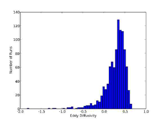
Figure 1: Statistics of eddy diffusivity.

In figure 2, the fields corresponding to one of the generated steady states are presented. The short-scale growth rates are $\lambda_{short}=-0.5662$, for symmetric perturbations, and $\lambda_{short}=-0.05175$, for antisymmetric perturbations. The maximum and minimum growth rates of large-scale perturbations are $\lambda_{2}^{max}=1.426$, for $\theta^{max}=3.392$, and $\lambda_{2}^{min}=-1.165$, for $\theta^{min}=3.593$, respectively. The maximum growth rate is positive (which corresponds to a negative eigenvalue of the eddy diffusivity tensor), i.e. a large-scale instability is present. All the auxiliary problems show a decaying energy spectrum (see figures 3-8 below) and the expected symmetries can be observed.

Spatial short-scale structure of the large-scale eigenmode is defined by the leading term $\mathbf{W}^{(0)}$ in the expansion (20), and therefore by the fields $\mathbf{S}_{i}$ (see (49)). Magnetic field in all of them (see figures 3-6) has the form of distorted "retrograde columns" (spie93, ) and concentrates near the horizontal boundaries of the layer. This kind of structure is reproduced in their linear combination $\mathbf{W}^{(0)}$ for the most unstable mode (see figure 7). Such behaviour was originally noticed in the non-linear evolutionary simulations (spie93, ) of magnetic field generation by rotating thermal convection, and it can be attributed to the boundary conditions, namely, ideal electric conductivity of the boundaries. It is interesting that this feature is quite robust – from the formal point of view our problem is evidently quite different from the one considered in (spie93, ).

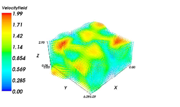
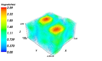
Steady state velocity	Steady state magnetic field
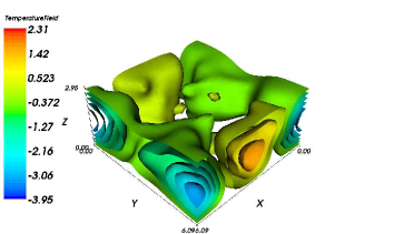
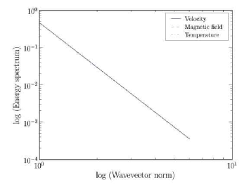
Steady state temperature	Steady state energy spectra

Figure 2: Basic (steady state) fields and corresponding energy spectra. Symmetry about the $z\mbox{-axis}$ is observed in all of the displayed fields.

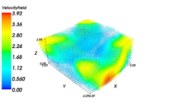
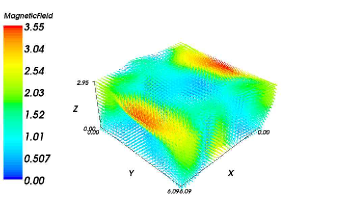
$\mathbf{S}_{1}:$ velocity	$\mathbf{S}_{1}:$ magnetic field
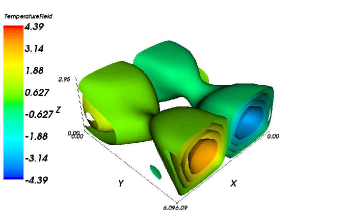
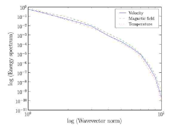
$\mathbf{S}_{1}:$ temperature	$\mathbf{S}_{1}:$ energy spectra

Figure 3: $\mathbf{S}_{1}$ fields and corresponding energy spectra. Anti-symmetry about the $z\mbox{-axis}$ is observed in all of the displayed fields.

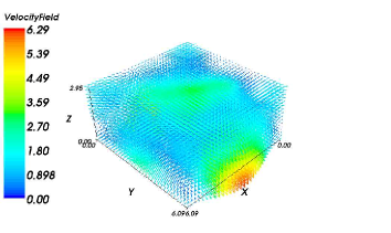
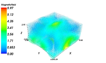
$\mathbf{S}_{2}:$ velocity	$\mathbf{S}_{2}:$ magnetic field
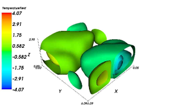
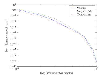
$\mathbf{S}_{2}:$ temperature	$\mathbf{S}_{2}:$ energy spectra

Figure 4: $\mathbf{S}_{2}$ fields and corresponding energy spectra. Anti-symmetry about the $z\mbox{-axis}$ is observed in all of the displayed fields.

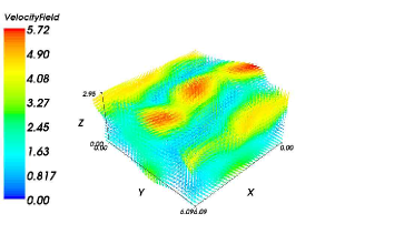
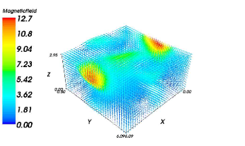
$\mathbf{S}_{3}:$ velocity	$\mathbf{S}_{3}:$ magnetic field
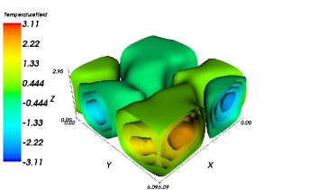
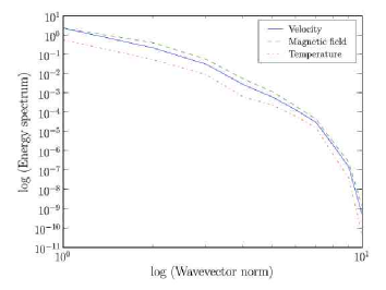
$\mathbf{S}_{3}:$ temperature	$\mathbf{S}_{3}:$ energy spectra

Figure 5: $\mathbf{S}_{3}$ fields and corresponding energy spectra. Anti-symmetry about the $z\mbox{-axis}$ is observed in all of the displayed fields.

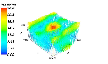
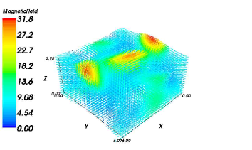
$\mathbf{S}_{4}:$ velocity	$\mathbf{S}_{4}:$ magnetic field
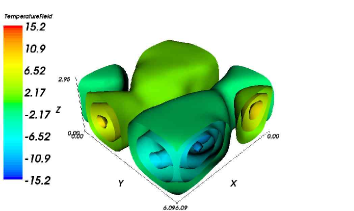
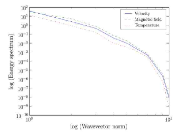
$\mathbf{S}_{4}:$ temperature	$\mathbf{S}_{4}:$ energy spectra

Figure 6: $\mathbf{S}_{4}$ fields and corresponding energy spectra. Anti-symmetry about the $z\mbox{-axis}$ is observed in all of the displayed fields.

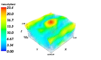
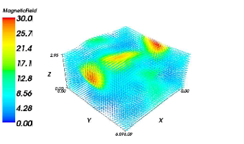
$\mathbf{W}^{(0)}:$ velocity	$\mathbf{W}^{(0)}:$ magnetic field
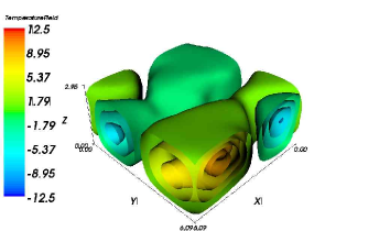
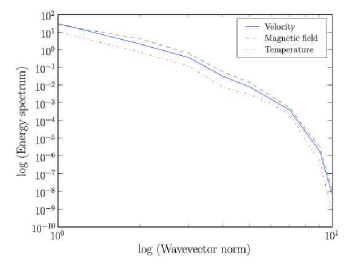
$\mathbf{W}^{(0)}:$ temperature	$\mathbf{W}^{(0)}:$ energy spectra

Figure 7: Short-scale structure of $\mathbf{W}^{(0)}$, for $\lambda_{2}^{max}$. Anti-symmetry about the $z\mbox{-axis}$ is observed in all of the displayed fields.

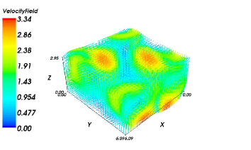
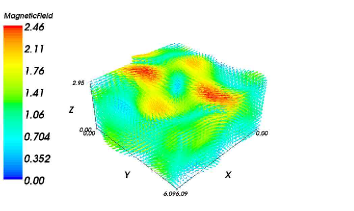
$\mathbf{\Gamma}_{11}:$ velocity	$\mathbf{\Gamma}_{11}:$ magnetic field
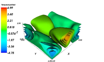
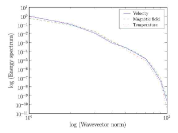
$\mathbf{\Gamma}_{11}:$ temperature	$\mathbf{\Gamma}_{11}:$ energy spectra

Figure 8: $\mathbf{\Gamma}_{11}$ fields and corresponding energy spectra. Symmetry about the $z\mbox{-axis}$ is observed in all of the displayed fields.

5 Concluding Remarks

We have derived an eigenvalue equation for large-scale perturbation modes of a CHM steady state. On average (over small spatial scales) the modes are, in the leading order, simple harmonic waves. Their growth rates are controlled by the combined diffusivity tensor, involving molecular kinematic viscosity and magnetic diffusivity and an additional tensor – the so-called combined eddy (turbulent) diffusivity correction, which is anisotropic (the entries of the matrix $\mathbf{E}^{\prime}$ depend on the direction of the wave vector $\mathbf{q}$), and which intermixes the influence of the flow and magnetic field. Originally this mutual influence is due to advection (the influence of the flow on magnetic field) and the action of the Lorentz force (the influence of the magnetic field on the flow), but it has now a different algebraic form – in particular, unlike in these basic physical laws, it is, on average, linear.

We have found that about $10\%$ of randomly generated steady CHM regimes, that are stable to short-scale perturbations, exhibit negative eddy diffusivity; such steady states are unstable to large-scale perturbations. However, the growth rate of the perturbation is quadratic in the scale ratio $\varepsilon$, i.e. it is small. Thus, this instability can be observed only if the considered CHM steady state is stable to short-scale perturbations, which would have larger ($O(\varepsilon^{0})$) growth rates otherwise. Other competing linear instabilities may also persist. For instance, in thermal convection in a rotating layer with free boundaries (with no magnetic field present), steady rolls, steady square cells, standing and travelling waves near the onset were demonstrated (Po05, ; Po05mjg, ) to be unstable to large-scale perturbations of a particular form (the small angle instability), with the growth rates scaling as $O(\varepsilon^{2})$ for the rolls and the cells, and $O(\varepsilon)$ for the waves (here $\varepsilon$ is the smallest scale ratio in the system); the rolls and square cells possess symmetry about the vertical axis.

The restriction that the perturbed CHM state is steady can be lifted (Zhe05fz, ). Instead of averaging over fast spatial variables, averaging over the spatio-temporal domain of fast variables must then be performed. This allows, in particular, to carry out the stability analysis of time-periodic CHM states. However, in any case the perturbed states are required to be symmetric (for instance, symmetry about the vertical axis, as considered here). Parity invariance is another type of symmetry consistent with the CHM equations, if the Joule term is neglected. Like the symmetry about the vertical axis, it guarantees that no $\alpha$-effect emerges and it allows to construct a second order combined eddy diffusivity operator by the same method of homogenisation.

Different multiscale expansions are obtained for different sets of conditions imposed at the horizontal boundaries of the layer. Often considered alternative boundary conditions include the no-slip condition for the flow, an isolator outside the fluid layer condition for the magnetic field, and heat insulating boundaries (zero heat flux condition) for temperature. They can be of interest, for instance, in geophysical applications (for which the no-slip condition at the outer kernel boundaries and the isolator condition at the outer boundary of the spherical layer are more appropriate than those considered here). The method of homogenisation that we have used relies on the existence of constant vector fields in $\textrm{ker}(\mathbf{P}\mathbf{A}^{(0)^{*}}\mathbf{P})$. In addition to the two constant horizontal vectors in the flow and magnetic field components considered here, another scalar constant, a fixed temperature, belongs to $\textrm{ker}(\mathbf{P}\mathbf{A}^{(0)^{*}}\mathbf{P})$, if Joule heating is neglected ($\sigma=0$) and the zero heat flux condition for temperature is assumed. Therefore, the procedure of homogenisation that we have used can be applied if, at least, one of the following conditions is imposed on the horizontal boundaries: free boundaries, or conducting boundaries, or no heat flux. Each quantity, satisfying boundary conditions from this list, increases dimension of the problem for large-scale mean-fields obtained from the solvability condition for the equations emerging at order 2. The remaining ones (temperature in the particular case that we have considered here) are essentially short-scale and only affect, via solutions of auxiliary problems at orders 0 and 1, the values of coefficients in the combined eddy diffusivity tensor for the large-scale quantities. The boundary conditions for which this approach is not directly applicable (i.e. the no-slip boundary condition for the flow, or the insulator condition for the magnetic field, or fixed temperature) can apparently still be treated by the homogenisation method that we have applied, but this requires considering boundary layers, increasing significantly the complexity of the problem.

A common feature of astrophysical convective systems, such as interiors of planets or stars, is rotation. A straightforward incorporation of the Coriolis force in the analysis is inconsistent with the homogenisation procedure that we have used: averaging of the linearised Navier-Stokes equation (for the free boundary conditions) shows that constant average non-zero horizontal velocities give rise to a non-zero average Coriolis force, which can be balanced only by a constant gradient of pressure. This suggests an unbounded linear growth of pressure, which is not, however, unphysical: in a rotating system only pressure can offset the centrifugal force. The simplest way to overcome the resultant algebraic difficulties is to consider the vorticity equation, for which the methods for construction of the two-scale expansion are applicable without any modifications.

Acknowledgements

We have benefited from stimulating discussions with U. Frisch, A.M. Soward and K. Zhang. MB was financially supported by FCT (Portugal, studentship BD/8453/2002). VZ is grateful to the Royal Society, the French Ministry of Education, CMAUP (Portugal) and the Russian Foundation for Basic Research (grant 04-05-64699).

References

- (1) R.T. Merrill, M.W. McEllhiny, P.L. McFadden, The magnetic field of the Earth. Paleomagnetism, the core and the deep mantle. (Academic Press, 1996)
- (2) E.R. Priest, Solar Magneto-Hydrodynamics (D.Reidel, 1984)
- (3) A.A. Ruzmaikin, D.D. Sokoloff, A.M. Shukurov, Magnetic Fields of Galaxies (Nauka, 1988), in Russian
- (4) H.K. Moffatt, Magnetic field generation in electrically conducting fluids (Cambridge University Press, 1978), ISBN 0-521-21640-0
- (5) E.N. Parker, Cosmical magnetic fields (Clarendon Press, 1979)
- (6) Y.B. Zeldovich, A.A. Ruzmaikin, D.D. Sokoloff, Magnetic Fields in Astrophysics (Gordon and Breach, 1983)
- (7) A.D. Polyanin, V.F. Zaytsev, Handbook of nonlinear equations of mathematical physics (Fizmatlit, 2002), in Russian
- (8) C.A. Jones, P.H. Roberts, J. Fluid Mech. 404, 311 (2000)
- (9) P.H. Roberts, C.A. Jones, Geophys. Astrophys. Fluid Dynam. 92, 289 (2000)
- (10) C.A. Jones, P.H. Roberts, Geophys. Astrophys. Fluid Dynam. 93, 173 (2000)
- (11) G.A. Glatzmaier, P.H. Roberts, Phys. Earth Planet. Inter. 91, 63 (1995)
- (12) G.A. Glatzmaier, P.H. Roberts, Nature 377, 203 (1995)
- (13) G.A. Glatzmaier, P.H. Roberts, Science 274, 1887 (1996)
- (14) G.A. Glatzmaier, P.H. Roberts, Physica D 97, 81 (1996)
- (15) G.A. Glatzmaier, P.H. Roberts, Contemporary physics 38, 269 (1997)
- (16) G.A. Glatzmaier, P.H. Roberts, Geowissenschaften 15, 95 (1997)
- (17) P.H. Roberts, G.A. Glatzmaier, Geophys. Astrophys. Fluid Dynam. 94, 47 (2001)
- (18) C.A. Jones, Phil. Trans. R. Soc. Lond. A 358, 873 (2000)
- (19) Y. Ponty, A.D. Gilbert, A.M. Soward, J. Fluid Mech. 435, 261 (2001)
- (20) Y. Ponty, A.D. Gilbert, A.M. Soward, in Dynamo and dynamics, a mathematical challenge., edited by P. Chossat, D. Armbruster, I. Oprea (Kluwer Academic Publishers, 2001), pp. 261–287
- (21) Y. Ponty, A.D. Gilbert, A.M. Soward, J. Fluid Mech. 487, 91 (2003)
- (22) J. Rotvig, C.A. Jones, Phys. Rev. E 66 (2002), [http://link.aps.org/abstract/PRE/v66/e056308]
- (23) S. Stellmach, U. Hansen, Phys. Rev. E 70(5) (2004), http://link.aps.org/abstract/PRE/v70/e056312]
- (24) K. Zhang, C.A. Jones, Geophys. Res. Lett. 24, 2869 (1997)
- (25) G.R. Sarson, C.A. Jones, Phys. Earth Planet. Inter. 111, 3 (1999)
- (26) K. Zhang, G. Schubert, Ann. Rev. Fluid Mech. 32, 409 (2000)
- (27) F. Busse, Ann. Rev. Fluid Mech. 32, 383 (2000)
- (28) U.R. Christensen, in Mantle convection. Plate tectonics and global dynamics. (Gordon and Breach Science Publishers, 1989), pp. 595–656
- (29) W.R. Peltier, in Mantle convection. Plate tectonics and global dynamics., edited by W.R.Peltier (Gordon and Breach Science Publishers, 1989), pp. 389–478
- (30) U. Christensen, P. Olson, G.A. Glatzmaier, Geophys. J. Int. 138(2), 393 (1999)
- (31) A. Bensoussan, J.L. Lions, G. Papanicolaou, Asymptotic Analysis for Periodic Structures (North Holland, 1978)
- (32) A. O.A.Oleinik, G.A.Yosifian, Mathematical problems in elasticity and homogenization (Elsevier Science Publishers, 1992)
- (33) V.V. Jikov, S.M. Kozlov, O.A. Oleinik, Homogenization of differential operators and integral functionals (Springer-Verlag, Berlin, 1994)
- (34) D. Cioranescu, P. Donato, An introduction to homogenization (Oxford Univ. Press, 1999)
- (35) U. Frisch, Z.S. She, P.L. Sulem, Physica D 28, 382 (1987)
- (36) P.L. Sulem, Z.S. She, H. Scholl, U. Frisch, J. Fluid Mech. 205, 341 (1989)
- (37) V.A. Zheligovsky, Geophys. Astrophys. Fluid Dynam. 59, 235 (1991)
- (38) V.P. Starr, Physics of negative viscosity phenomena (McGraw-Hill, 1968)
- (39) G. Sivashinsky, V. Yakhot, Phys. Fluids. 28, 1040 (1985)
- (40) G.I. Sivashinsky, A.L. Frenkel, Phys. Fluids. A 4, 1608 (1992)
- (41) S. Gama, M. Vergassola, U. Frisch, J. Fluid Mech. 260, 95 (1994)
- (42) V.I. Yudovich, Mehanika zhidkosti i gaza (4) 25(4), 31 (1990), in Russian
- (43) B. Dubrulle, U. Frisch, Phys. Rev. A 43, 5355 (1991)
- (44) A. Wirth, S. Gama, U. Frisch, J. Fluid Mech. 288, 249 (1995)
- (45) A. Wirth, Physica D 76, 312 (1994)
- (46) L. Biferale, A. Crisanti, M. Vergassola, A. Vulpiani, Phys. Fluids 7, 2725 (1995)
- (47) M. Vergassola, M. Avellaneda, Physica D. 106, 148 (1997)
- (48) S. Childress, J. Math. Phys. 11, 3063 (1970)
- (49) A.M. Soward, Phil. Trans. R. Soc. Lond. A 275, 611 (1974)
- (50) M.M. Vishik, in Mathematical methods of seismology and geodynamics. Comp. seismol. (Nauka, 1986), Vol. 19, pp. 186–215, in Russian
- (51) M.M. Vishik, in Numerical modelling and analysis of geophysical processes. Comp. seismol. (Nauka, 1987), Vol. 20, pp. 12–22, in Russian
- (52) A. Lanotte, A. Noullez, M. Vergassola, A. Wirth, Geophys. Astrophys. Fluid Dynam. 91, 131 (1999)
- (53) V.A. Zheligovsky, O.M. Podvigina, U. Frisch, Geophys. Astrophys. Fluid Dynam. 95, 227 (2001), [http://xxx.lanl.gov/abs/nlin.CD/0012005]
- (54) V.I. Yudovich, Izvestiya vuzov. Severo-Kavkazskiy region. Estestvennye nauki. Specvypusk. pp. 155–160 (2001), in Russian
- (55) V.A. Zheligovsky, O.M. Podvigina, Geophys. Astrophys. Fluid Dynam. 97, 225 (2003), [http://xxx.lanl.gov/abs/physics/0207112]
- (56) V.A. Zheligovsky, Geophys. Astrophys. Fluid Dynam. 99, 151 (2005)
- (57) V.A. Zheligovsky, Izvestiya, Physics of the Solid Earth 39(5), 409 (2003)
- (58) O.M. Podvigina, Submitted to Geophys. Astrophys. Fluid Dynam. (2005)
- (59) O.M. Podvigina (2005), submitted to Mechanics of fluid and gas (in Russian). (English translation: Fluid Dynamics, 2005).
- (60) S.M. Cox, P.C. Matthews, J. Fluid Mech. 403, 153 (2000)
- (61) Y. Ponty, T. Passot, P. Sulem, Phys. Rev. E 56, 4162 (1997)
- (62) V.A. Zheligovsky (2005), submitted to Fizika Zemli, 2005 (in Russian). (English translation: Izvestiya, Physics of the Solid Earth, 2005).
- (63) S. Chandrasekhar, Hydrodynamic and Hydromagnetic Stability (Dover Publications, Inc., 1981)
- (64) F. Riesz, B. Sz.-Nagy, Functional Analysis (Dover, 1990)
- (65) O. Axelson, Iterative solution methods (Cambridge University Press, 1998), ISBN 0-521-55569-8
- (66) V. Zheligovsky, J. of Scientific Computing 8(1), 41 (1993)
- (67) M.G. St. Pierre, in Solar and Planetary Dynamos, edited by M. Proctor, P.C. Matthews, A.M. Rucklidge (Cambridge Univ. Press, 1993), pp. 295–302