2-Soliton-solution of the Novikov-Veselov equation

J. Nickel, H. W. Schürmann

Based on a superposition method recently proposed to obtain 1-solitary wave solutions of the KdV-Burgers equation [Yuanxi et al. 2005], we show that this method can also be used to find a 2-solitary wave solution of the Novikov-Veselov equation. Thus, it seems that the method of Yuanxi and Jiashi in general is not restricted to constructing 1-solitary wave solutions of nonlinear wave and evolution equations (NLWEEs).

KEY WORDS: Linear superposition; solitary wave solution, Novikov-Veselov equation.
PACS: 02.30.Jr

1 Introduction

We analyze the Novikov-Veselov equation (NV equation) given by Hu [Hu 1994] which is another (2 + 1)-dimensional analog of the KdV equation besides the well-known Kadomtsev-Petviashvili equation [Cheng 1990]. It has relevance in nonlinear physics (in particular in inverse scattering theory) [Tagami 1989, Cheng 1990, Athorne et al. 1991, Hu 1994, Hu et al. 1996, Konopelchenko et al. 1996] and mathematics (cf. e.g. [Taimanov 1995, Ferapontov 1999]). To obtain a 2-soliton solution of the NV equation Hu has developed a nonlinear superposition formula [Hu 1994, Eq. (5)]. In the following we show that a 2-solitary wave solution of the NV equation can even be obtained by a linear superposition method given by Yuanxi and Jiashi [Yuanxi et al. 2005] that was proposed to find 1-solitary wave solutions of nonlinear wave and evolution equations.

2 2-soliton solution of the NV equation obtained by linear superposition

We consider the following equations

$$U_{t}+U_{xxx}+3\left(U^{2}\right)_{x}=0,$$ (1)

$$U_{t}+U_{yyy}+3\left(U^{2}\right)_{y}=0,$$ (2)

$$2U_{t}+U_{xxx}+U_{yyy}+3(U\>\partial_{y}^{-1}U_{x})_{x}+3(U\>\partial_{x}^{-1}U_{y})_{y}=0.$$ (3)

Obviously, the KdV equation (1), (2) and the NV equation (3) are related: The linear terms of Eq. (3) are equal to the superposition of those of Eq. (1) and Eq. (2) and the nonlinear terms of Eq. (3) are equal to the superposition of those of Eqs. (1) and (2) if traveling waves are considered with $\partial_{x}^{-1}=\partial_{y}^{-1}$. Following the ideas of Yuanxi and Jiashi [Yuanxi et al. 2005] we construct the solutions of Eq. (3) by linear superposition of those to Eq. (1) and Eq. (2).

According to a method described by Schürmann and Serov [Schürmann et al. 2004] we can evaluate the following 1-solitary wave solutions of Eqs. (1), (2)

$$U(x,t) = \frac{c}{2\>k}\mathrm{sech}^{2}\left[\frac{1}{2}\sqrt{\frac{c}{k^{3}}}(kx-ct-y_{0})\right],$$ (4)

$$U(y,t) = \frac{c}{2\>k}\mathrm{sech}^{2}\left[\frac{1}{2}\sqrt{\frac{c}{k^{3}}}(ky-ct-x_{0})\right],$$ (5)

where $x_{0}$ and $y_{0}$ are arbitrary constants. Combining these solutions and choosing $k=1$, so that $\partial_{x}^{-1}=\partial_{y}^{-1}$,

$$U(x,y,t)=\frac{c}{2}\mathrm{sech}^{2}\left[\frac{1}{2}\sqrt{c}\>(x+y-ct)\right]$$ (6)

is a 1- solitary wave solution of Eq. (3).
We tentatively write a 2-solitary wave solution according to

$$U(x,y,t) = a\>\mathrm{sech}^{2}\left[\frac{1}{2}\sqrt{c}\>(k_{1}x+p_{1}y-ct)\right]+b\>\mathrm{sech}^{2}\left[\frac{1}{2}\sqrt{c}\>(k_{2}x+p_{2}y-ct)\right],$$

$$z_{i} = \frac{1}{2}\sqrt{c}\>(k_{i}x+p_{i}y-ct),\>i\in\{1,2\},$$ (7)

with $c>0$ and $a,\>b,\>k_{1},\>k_{2},\>p_{1},\>p_{2}$ to be determined. Inserting Eq. (2) into Eq. (3) leads to

$$\frac{2\>a\>\sqrt{c}\>\mathrm{sech}^{2}z_{1}\mathrm{tanh}z_{1}}{4k_{1}k_{2}p_{1}p_{2}} \left(-2ck_{1}k_{2}p_{1}p_{2}(k_{1}^{3}+p_{1}^{3}-2)-6k_{2}p_{2}(2a-ck_{1}p_{1})(k_{1}^{3}+p_{1}^{3})\mathrm{sech}^{2}z_{1}\right)$$ (8)

$$-\frac{2\>a\>\sqrt{c}\>\mathrm{sech}^{2}z_{1}\mathrm{tanh}z_{1}}{4k_{1}k_{2}p_{1}p_{2}} (6b(k_{2}p_{1}+k_{1}p_{2})(k_{1}^{2}k_{2}+p_{1}^{2}p_{2})\>\textrm{sech}^{2}z_{2})$$

$$+\frac{2\>b\>\sqrt{c}\>\mathrm{sech}^{2}z_{2}\mathrm{tanh}z_{2}}{4k_{1}k_{2}p_{1}p_{2}} \left(-2ck_{1}k_{2}p_{1}p_{2}(k_{2}^{3}+p_{2}^{3}-2)-6k_{1}p_{1}(2b-ck_{2}p_{2})(k_{2}^{3}+p_{2}^{3})\mathrm{sech}^{2}z_{2}\right)$$

$$-\frac{2\>b\>\sqrt{c}\>\mathrm{sech}^{2}z_{2}\mathrm{tanh}z_{2}}{4k_{1}k_{2}p_{1}p_{2}} (6a(k_{2}p_{1}+k_{1}p_{2})(k_{1}k_{2}^{2}+p_{1}p_{2}^{2})\>\textrm{sech}^{2}z_{1})=0.$$

Assuming $\frac{2\>a\>\sqrt{c}\>\mathrm{sech}^{2}z_{1}\mathrm{tanh}z_{1}}{4k_{1}k_{2}p_{1}p_{2}}\neq 0$ and $\frac{2\>b\>\sqrt{c}\>\mathrm{sech}^{2}z_{2}\mathrm{tanh}z_{2}}{4k_{1}k_{2}p_{1}p_{2}}\neq 0$ and setting the coefficients of $\mathrm{sech}^{2}z_{i}$ equal to zero we obtain

$$a = \lambda_{1}\frac{cp_{2}(p_{2}^{3}-2)^{\frac{1}{3}}}{2(p_{2}^{3}-1)^{\frac{2}{3}}},b=-\frac{1}{2}\lambda_{2}cp_{2}(p_{2}^{3}-2)^{\frac{1}{3}},k_{1}=\lambda_{3}\left(2-\frac{p_{2}^{3}}{p_{2}^{3}-1}\right)^{\frac{1}{3}},$$ (9)

$$k_{2} = -\lambda_{4}(p_{2}^{3}-2)^{\frac{1}{3}},p_{1}=\lambda_{5}\frac{p_{2}}{(p_{2}^{3}-1)^{\frac{1}{3}}}\>\>\>\>\>\>\textrm{with}$$

	$\lambda_{1}$	$\lambda_{2}$	$\lambda_{3}$	$\lambda_{4}$	$\lambda_{5}$
I	$1$	$1$	$1$	$1$	$1$
II	$1$	$-(-1)^{\frac{1}{3}}$	$(-1)^{\frac{2}{3}}$	$-(-1)^{\frac{1}{3}}$	$-(-1)^{\frac{1}{3}}$
III	$1$	$(-1)^{\frac{2}{3}}$	$-(-1)^{\frac{1}{3}}$	$(-1)^{\frac{2}{3}}$	$(-1)^{\frac{2}{3}}$
IV	$-(-1)^{\frac{1}{3}}$	$1$	$(-1)^{\frac{2}{3}}$	$1$	$(-1)^{\frac{2}{3}}$
V	$-(-1)^{\frac{1}{3}}$	$-(-1)^{\frac{1}{3}}$	$-(-1)^{\frac{1}{3}}$	$-(-1)^{\frac{1}{3}}$	$1$
VI	$-(-1)^{\frac{1}{3}}$	$(-1)^{\frac{2}{3}}$	$1$	$(-1)^{\frac{2}{3}}$	$-(-1)^{\frac{1}{3}}$
VII	$(-1)^{\frac{2}{3}}$	$1$	$-(-1)^{\frac{1}{3}}$	$1$	$-(-1)^{\frac{1}{3}}$
VIII	$(-1)^{\frac{2}{3}}$	$-(-1)^{\frac{1}{3}}$	$1$	$-(-1)^{\frac{1}{3}}$	$(-1)^{\frac{2}{3}}$
IX	$(-1)^{\frac{2}{3}}$	$(-1)^{\frac{2}{3}}$	$(-1)^{\frac{2}{3}}$	$(-1)^{\frac{2}{3}}$	1

New solutions are given if $p_{2}\in\mathbb{R}$ can be chosen so that $k_{i}$ and $p_{1}$ are real, $a$ and $b$ may be complex. Subject to certain conditions some of these solutions are even physical (real and bounded) solutions. As an example the solution

$$U(x,y,t) = \frac{cp_{2}(p_{2}^{3}-2)^{1/3}}{2(p_{2}^{3}-1)^{2/3}}\mathrm{sech}^{2}\left(\frac{\sqrt{c}(p_{2}y+(p_{2}^{3}-2)^{1/3}x-c(p_{2}^{3}-1)^{1/3}t)}{2(p_{2}^{3}-1)^{1/3}}\right)$$ (11)

$$- \frac{cp_{2}(p_{2}^{3}-2)^{1/3}}{2}\mathrm{sech}^{2}\left(\frac{\sqrt{c}}{2}(-p_{2}y+(p_{2}^{3}-2)^{1/3}x+ct)\right),$$

$$p_{2}>\sqrt[3]{2}$$

(according to Eqs. (2), (9) and line I of the above table) is shown in Fig. 1. We have verified this solution by putting it into the original equation (3) utilizing Mathematica.

3 Summary and concluding remarks

By analyzing the structure of the NV equation we have shown that by using a superposition method proposed to construct 1-solitary wave solutions of NLWEEs 2-solitary wave solutions can be obtained. We suppose that the technique of Yuanxi and Jiashi [Yuanxi et al. 2005] may lead to multi-solitary wave solutions of certain NLWEEs if the NLWEE in quesion can be considered as a superposition of NLWEEs that have the same type of solitary wave solution (e.g., $\mathrm{sech}^{2}$); we leave this to future study.

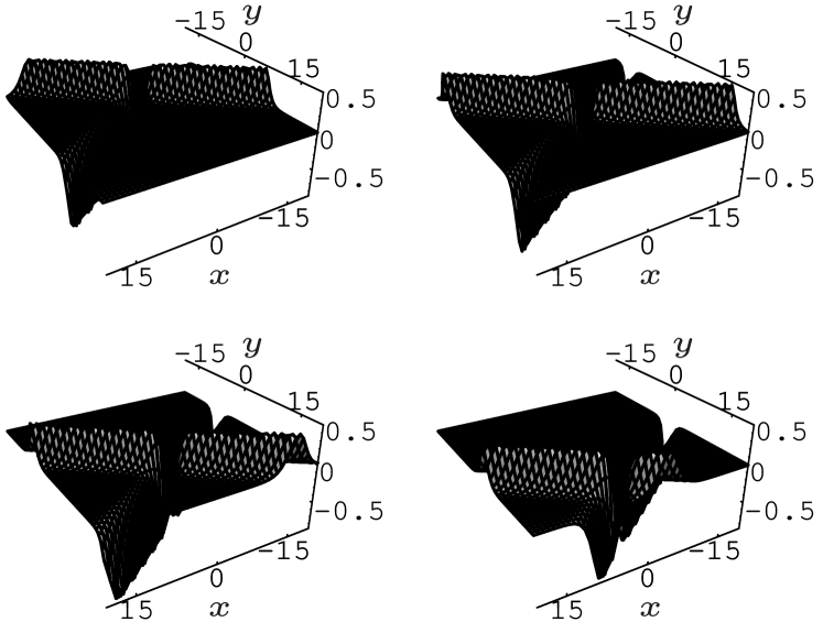
Figure 1: 2-soliton solution (cf. Eq. (2), I ) for $t=-10,0,10,20$ ($c=1$, $p_{2}=1.5$).

References

- [Athorne et al. 1991] Athorne C. and Nimmo J. J. C (1991), Inverse Problems 7, 809-826.
- [Cheng 1990] Cheng Y. (1990), J. Math. Phys. 32, 157-162.
- [Ferapontov 1999] Ferapontov E. V. (1999), Differential Geometry and its Applications 11, 117-128.
- [Hu 1994] Hu X.-B. (1994), J. Phys. A: Math. Gen. 27, 1331-1338.
- [Hu et al. 1996] Hu X.-B. and Willox R. (1996), J. Phys. A.: Math. Gen. 29, 4589-4592.
- [Konopelchenko et al. 1996] Konopelchenko B. and Moro A. (2004), J. Phys. A: Math. Gen. 37, L105-L111.
- [Schürmann et al. 2004] Schürmann H. W. and Serov V. S. (2004), Proc. Progress in Electromagnetics Research Symposium March 28-31 (Pisa), 651-654.
- [Tagami 1989] Tagami Y. (1989) arXiv: dg-ga/9511005 v5 20 Nov 1995.
- [Taimanov 1995] Taimanov I. A. (1995), Phys. Lett. A 141, 116-120.
- [Yuanxi et al. 2005] Yuanxi X. and Jiashi T. (2005), International Journal of Theoretical Physics 44, 293-301.