The Size of Ghost Rods

Abstract

‘Ghost Rods’ are periodic structures in a two-dimensional flow that have an effect on material lines that is similar to real stirring rods. An example is a periodic island: material lines exterior to it must wrap around such an island, because determinism forbids them from crossing through it. Hence, islands act as topological obstacles to material lines, just like physical rods, and lower bounds on the rate of stretching of material lines can be deduced from the motion of islands and rods. Here, we show that unstable periodic orbits can also act as ghost rods, as long as material lines can ‘fold’ around the orbit, which requires the orbit to be parabolic. We investigate the factors that determine the effective size of ghost rods, that is, the magnitude of their impact on material lines.

To be published in ‘Proceedings of the Workshop on Analysis and Control of Mixing with Applications to Micro and Macro Flow Processes,’ CISM, Udine, Italy, July 2005. (Springer-Verlag, 2006)

Chapter 1 Introduction

Topological kinematics is the application of topology to chaotic advection in fluids. In two dimensions, braids are the natural mathematical construct to use for a topological analysis. Boyland et al. used braids very effectively to analyse the motion of stirring rods in viscous flow (Boyland et al., 2000) and point vortices in ideal flow (Boyland et al., 2003). A braid is associated with the motion of the rods or vortices by plotting their trajectory in a space-time diagram: the resulting “spaghetti plot” is obviously a braid. Here, we shall not be too concerned with the precise mathematical properties of braids—the intuitive, capillary notion of what a braid resembles will suffice.

Rods and points vortices share the common feature that they are topological obstacles to material lines in two dimensions. Of course, any fluid particle is such an obstacle, and recently one of us analysed braids formed by particle trajectories (Thiffeault, 2005). The fact that particle orbits are topological obstacles puts a lower bound on the topological entropy—the growth rate of material lines (Boyland et al., 2000; Newhouse and Pignataro, 1993). Imagine a material line that is initially linked around the topological obstacles under consideration (rods or fluid particles). Then as the position of these obstacles evolves the material line is dragged along, and as the particles braid around each other the material line must grow by at least a certain amount. The properties of the braid thus imply a lower bound on the growth rate of material lines in the fluid.

For time-periodic flows, the natural topological obstacles to study are fluid parcels associated with particular periodic orbits. Recently, we introduced to fluid mechanics the concept of “ghost rods” (Gouillart et al., 2005). We analysed the motion of material rods, stable periodic orbits (islands), and unstable periodic orbits from a topological perspective. We showed that periodic orbits associated with islands behave very similarly to material rods: they are large topological obstacles ploughing through the fluid, and material lines must get out of their way or else wrap around them. Periodic islands have the advantage of being easily identifiable visually, and can clearly be regarded as “rods.” Figure 1 illustrates this: there is only one physical rod stirring the flow, but a ghostly second rod is clearly visible in the centre-left portion of the plot, around which material lines are wrapped.

Figure 1: A material line being stirred by a moving rod in a viscous fluid. The rod is the circle visible in the centre-right portion of the fluid, but observe that there is a rod-like structure in the centre-left portion. This is a periodic island that acts like a rod—a ghost rod.

Indeed, there is a regular island in that region (Gouillart et al., 2005).

The foregoing description is topological in nature. The size of the rods is immaterial to the topological entropy (Boyland et al., 2000; Finn et al., 2003). Of course, in practice their size matters a lot: if the rods are made smaller, so does the region of the fluid for which the topological entropy lower bound applies. In the limit of infinitely small rods, one might expect this region to shrink to zero. This is certainly true of physical rods: if they were made infinitely small, the fluid would not even notice their presence and nothing would happen, except in a vanishingly small region. There is currently no theory that gives the size of the affected region given the size of the rods and their path, but in practice it is observed (in viscous flows) that it is of the order of the size of the rods and the size of the region swept by their motion.

So much for physical rods. But what about ghost rods? As their name indicates, they have no material existence. However, since they behave much like physical rods, we may ask what is their effective size. That is, topologically a ghost rod is supposed to mimic a real physical rod, but how much of an impact does it effectively have on the surrounding fluid? For periodic islands, the answer is clear: the effective size of the ghost rod is the size of the island. Figure 1 convincingly illustrates that, as far as material lines are concerned, there is a stirring rod of the size of the periodic island in the centre-left portion of the flow.

For unstable periodic orbits, the answer is much less clear, since in principle ghost rods of this type have zero size. In this paper, we shall investigate the effective size of ghost rods associated with unstable periodic orbits. In fact, as we shall see, not all unstable periodic orbits can even be said to be ghost rods. Rather, only unstable periodic orbits of parabolic (as opposed to hyperbolic) type can hope to qualify as ghost rods. The local linear structure near an hyperbolic orbit prevents material lines from “wrapping” around the periodic point, so that it does not appear as a rod at all. For parabolic orbits of a certain type, the unstable manifold terminates at the periodic orbit, allowing material lines to wrap around the point without encountering the invariant manifold. Thus, the periodic orbit appears visually as a tiny rod, which is our criterion for considering periodic orbits to be ghost rods.

Chapter 2 Unstable Periodic Orbits

In an incompressible flow, the linearised flow around an unstable periodic orbit can be one of two types. Figure 2 depicts the most common, called a hyperbolic orbit, or hyperbolic point if one is speaking of the Poincaré section (stroboscopic map) of the time-periodic flow.

\psfrag{unstable}{unstable}\psfrag{stable}{stable}\includegraphics[width=115.23482pt]{hyper.eps}

Figure 2: The stable and unstable manifolds of a hyperbolic point.

There are two distinguished directions along which points respectively get away from or converge to the periodic orbit. These directions can be nonlinearly extended into the unstable and stable manifolds of the periodic orbit. A sufficient condition for the periodic orbit to be hyperbolic is that its Floquet matrix have nondegenerate eigenvalues. (The Floquet matrix is obtained by linearising the system about the periodic orbit and integrating over a full period of the orbit, as we will do in Section 3 for a specific flow.) Even though they are topological obstacles to material lines in the flow, such orbits can hardly be called ghost rods. This is because material lines must align with the unstable manifold of the periodic orbit, a phenomenon sometimes referred to as asymptotic directionality (Giona et al., 1998; Thiffeault, 2004). A material line cannot possibly fold around such a periodic orbit, since the unstable manifold goes straight through the orbit and appears linear in its neighbourhood. Hence, the periodic orbit does not “look” like a tiny little rod to the naked eye: it looks like any other point on the material line, and only a detailed knowledge of the velocity field allows its detection, usually by numerical means. We conclude that hyperbolic periodic orbits do not form “proper” ghost rods, since they cannot be detected visually.

That leaves the second type of unstable periodic orbit: parabolic orbits. In that case the Floquet matrix has degenerate eigenvalue that must both be equal to unity, by incompressibility of the fluid. For parabolic points, we cannot deduce the behaviour of points near the periodic orbit by examining only the linearised system—nonlinear terms must be considered. As we shall see in the following section, a particular type of nonlinear structure gives rise to parabolic points that exhibit the appropriate behaviour for a ghost rod.

Chapter 3 Case Study: The Sine Flow

We shall now illustrate the type of unstable periodic orbit that gives rise to ghost rods by examining a specific system, namely the Zeldovich sine flow (Pierrehumbert, 1994). This is a nice system to work with because its Poincaré map can be obtained analytically, and for special parameter values we can also determine some periodic orbits analytically. These orbits were exploited by Finn et al. (2005) to show the presence of chaos. The sine flow is given by the velocity field

$$\bm{u}(\bm{x},t)=\begin{cases}(0\,,\,\sin 2\pi x),\quad&n\tau\leq t<(n+\tfrac{1}{2})\tau;\\ (\sin 2\pi y\,,\,0),\quad&(n+\tfrac{1}{2})\tau\leq t<(n+1)\tau,\end{cases}$$ (1)

where $n$ is an integer. The equation $\dot{}\bm{x}=\bm{u}(\bm{x},t)$ can then be integrated over one period to give the sine map

$$\begin{split}x_{n+1}&=x_{n}+\tfrac{1}{2}\,\tau\,\sin 2\pi y_{n+1}\,;\\ y_{n+1}&=y_{n}+\tfrac{1}{2}\,\tau\,\sin 2\pi x_{n}\,,\end{split}$$ (2)

with $\bm{x}_{n}\mathrel{\raisebox{0.29707pt}{:}\!\!=}\bm{x}(n\tau)$. As an example, we will take $\tau=1$, because then we can determine many periodic orbits analytically. For instance, there is a period-4 orbit starting at $\bm{x}_{0}=(1/12,1/2)$, with iterates

$$(1/12,1/2)\rightarrow(7/12,3/4)\rightarrow(7/12,1/2)\rightarrow(1/12,1/4)\rightarrow(1/12,1/2).$$ (3)

The initial location of this orbit is inside the small square in Fig. 3, which also shows a material line advected for a few periods of the sine flow.

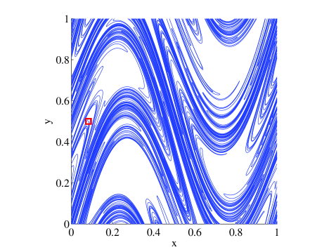
Figure 3: (a) A material line stretched and folded by the sine flow. The parabolic periodic point at $(x,y)=(1/12,1/2)$ is shown boxed. (b) Blow-up of the periodic point. Note that the material line is folded near, but not quite tightly around, the parabolic fixed point.

Figure 3 is a blow-up of the material line near this periodic orbit. Notice how the material line is sharply folded around the periodic orbit. In fact, Fig. 3 contains several such sharp folds. They are quite generic in chaotic flows, and are associated with regions of anomalously low stretching (Liu and Muzzio, 1996; Thiffeault, 2004).

We are interested in the behaviour of the map (2) in the neighbourhood of this periodic orbit, so we define a variable $\widetilde{\bm{X}}\mathrel{\raisebox{0.29707pt}{:}\!\!=}\bm{x}-\bm{x}_{0}$. Then, we can expand the map to second order in $\widetilde{\bm{X}}$,

$$\begin{split}\widetilde{X}^{\prime}&=\widetilde{X}-2\pi\widetilde{Y}+\alpha_{\widetilde{X}}\,\widetilde{X}^{2}+\beta_{\widetilde{X}}\,\widetilde{Y}^{2}+\gamma_{\widetilde{X}}\,\widetilde{X}\widetilde{Y},\\ \widetilde{Y}^{\prime}&=\widetilde{Y}\phantom{-2\pi\widetilde{Y}}\ \,+\alpha_{\widetilde{Y}}\,\widetilde{X}^{2}+\beta_{\widetilde{Y}}\,\widetilde{Y}^{2}+\gamma_{\widetilde{Y}}\,\widetilde{X}\widetilde{Y},\end{split}$$ (4)

where the primes denote four iterations of the sine map, so that the periodic orbit has become a fixed point of the map (4) at $\widetilde{\bm{X}}=(0,0)$. The periodic orbit is parabolic, as can easily be seen from the fact that the linear part of (4) (the Floquet matrix) has matrix representation

$$\mathcal{J}=\begin{pmatrix}1&-2\pi\\ 0&1\end{pmatrix},$$ (5)

which implies unit eigenvalues for the map. However, this matrix is not diagonalisable: it only has one eigenvector, $(0\ \ 1)^{T}$ (this can only occur for a parabolic point). We will see that it is this nondiagonalisable nature that allows the “folding” of material lines around the periodic point. In general, a matrix $\mathcal{J}$ has this property if $(\mathcal{J}-\mathbb{I})^{2}=0$, for $\mathcal{J}\neq\mathbb{I}$, which given that $\det\mathcal{J}=1$ is equivalent to $\operatorname{tr}\mathcal{J}=2$, with $\mathcal{J}\neq\mathbb{I}$.

After a linear transformation and a near-identity area-preserving quadratic transformation, Eq. 4 can be brought into the form

$$\begin{split}X^{\prime}&=X+Y+\alpha\,XY\,,\\ Y^{\prime}&=Y+\alpha\left(\tfrac{1}{2}X^{2}+XY\right),\end{split}$$ (6)

where the coefficients are such that the map is area-preserving to linear order. (The transformation used to get to (6) is not generally orientation-preserving.) As long as the linear part of the system is a Jordan block of the form (5), we can transform the system to Eq. (6). We have thus reduced the dynamics near the parabolic point to a one-parameter map (basically a Hénon map), which we proceed to analyse.

1 Invariant Manifolds and Dynamics Near the Origin

We now want to find the shape of the unstable and stable manifolds of the fixed point of (6) at the origin. Unlike hyperbolic fixed points, for a parabolic point the invariant manifolds cannot be determined solely from the linear part. Rather, we use the invariance property of the manifold: we parametrise the invariant manifold by $(X,Y_{\mathrm{inv}}(X))$ and iterate the map,

$$X^{\prime} =X+Y_{\mathrm{inv}}(X)+\alpha\,XY_{\mathrm{inv}}(X)\,,$$ (7a)

$$Y_{\mathrm{inv}}(X^{\prime}) =Y_{\mathrm{inv}}(X)+\alpha\left(\tfrac{1}{2}X^{2}+XY_{\mathrm{inv}}(X)\right),$$ (7b)

where we wrote $Y^{\prime}=Y_{\mathrm{inv}}(X^{\prime})$ since, by the invariance property, the iterated point must still belong to the invariant manifold. We can then substitute (7a) into (7b),

$$Y_{\mathrm{inv}}(X+Y_{\mathrm{inv}}(X)+\alpha\,XY_{\mathrm{inv}}(X))=Y_{\mathrm{inv}}(X)+\alpha\left(\tfrac{1}{2}X^{2}+XY_{\mathrm{inv}}(X)\right),$$ (8)

which is an equation that must be solved for $Y_{\mathrm{inv}}(X)$. We are interested in the small $X$ form of the manifold, so we assume $Y_{\mathrm{inv}}(X)=\sigma X^{\delta}$ and try to balance the leading order terms:

$$\sigma\,(X+\sigma X^{\delta}+\alpha\,\sigma X^{1+\delta})^{\delta}=\sigma X^{\delta}+\alpha\left(\tfrac{1}{2}X^{2}+\sigma X^{1+\delta}\right).$$ (9)

Where we go next depends on the magnitude of $\delta$. If $\delta=1$, we get the equation $\sigma(1+\sigma)=\sigma$ for the coefficients of the linear terms, which implies $\sigma=0$, an unacceptable state of affairs since then the quadratic term is unbalanced. If $\delta<1$, we get the leading balance

$$\sigma\,(\sigma X^{\delta})^{\delta}=\sigma X^{\delta}.$$ (10)

This can only be satisfied for $\delta=1$, a contradiction, or $\delta=0$, which again leads to an unbalanced quadratic term. Hence, our only choice is to take $\delta>1$, which gives the leading-order balance

$$\sigma\,(X+\sigma X^{\delta})^{\delta}=\sigma X^{\delta}+\tfrac{1}{2}\alpha X^{2},$$ (11)

where we have kept an extra order, because the leading terms cancel after expanding the exponent,

$$\sigma X^{\delta}\,(1+\sigma\delta X^{\delta-1})=\sigma X^{\delta}+\tfrac{1}{2}\alpha X^{2},$$ (12)

and we get finally

$$\sigma^{2}\,\delta X^{2\delta-1}=\tfrac{1}{2}\alpha X^{2},$$ (13)

yielding $\delta=3/2$, $\sigma=\pm\sqrt{\alpha/3}$. We can thus write the shape of the invariant manifolds as

$$Y_{\mathrm{inv}}(X)=\pm\sqrt{\tfrac{1}{3}\,\alpha X}X\,,$$ (14)

to leading order, where we have written $\alpha X$ under the square root to show that $X$ and $\alpha$ must have the same sign. Note an important fact: the manifolds exist only on one side of the $X$ axis, in contrast to Fig. 2 where the manifolds must radiate from the fixed point in four directions.

The two solutions for $\sigma$ correspond to the stable and unstable manifolds. We can determine which sign goes with which manifold by looking at an iterate of $X$ in Eq. (7a),

$$X^{\prime}=X\pm\sqrt{\tfrac{1}{3}\,\alpha X}X\,,$$ (15)

where we neglected higher-order terms ($X^{5/2}$). Thus, for $\alpha>0$, which implies $X>0$, the ‘$+$’ solution takes $X$ farther from the origin (unstable manifold), whilst the ‘$-$’ solutions takes the point closer to the origin (stable manifold). The situation is reversed for $\alpha<0$.

Figure 4 shows a few iterates of horizontal lines

\psfrag{it=0}{$\scriptstyle n=0$}\psfrag{it=7}{$\scriptstyle n=7$}\psfrag{it=14}{$\scriptstyle n=14$}\psfrag{it=21}{$\scriptstyle n=21$}\psfrag{it=28}{$\scriptstyle n=28$}\psfrag{it=35}{$\scriptstyle n=35$}\psfrag{it=42}{$\scriptstyle n=42$}\psfrag{it=49}{$\scriptstyle n=49$}\psfrag{it=56}{$\scriptstyle n=56$}\psfrag{X}{$X$}\psfrag{Y}{$Y$}\includegraphics[width=384.1122pt]{folditer.eps}

Figure 4: Iteration of a few material lines by the map (6) for $\alpha=1$. The lines fold around the unstable manifold (dashed curve). The $X$ axis has been rescaled by $10^{-3}$, the $Y$ axis by $10^{-4}$.

under the action of the map (6). The linear part of the map acts as a “shear flow” that sweeps the line around the origin, but the nonlinear terms prevent the line from crossing the unstable manifold. The net result is a line folded around the unstable manifold. This is why it is appropriate to refer to (6) as the ‘folding normal form’: inside every sharp fold of the flow lurks such a map. Since nearby material lines align with the unstable manifold of the periodic orbit, the folding is made possible by the one-sidedness of the unstable manifold: unlike hyperbolic points (Fig. 2), the manifold does not traverse the parabolic periodic point, but instead terminates there. This allows material lines to wrap around the periodic point without encountering the invariant unstable manifold, which cannot be crossed.

2 Curvature

As time progresses the folds in the material lines in Fig. 4 come closer and closer to the periodic orbit. There seems to be no limit to how close they can come, which is consistent with the ghost rod having zero effective size. The best we can do is to characterise the effective size of the ghost rod by how quickly the curvature of the folds evolve. We shall now examine how the curvature of a material line evolves near the parabolic orbit.

Consider a material line going through the origin of (6), as depicted in Fig. 4. The tangent map of (6) at the origin tells us how the tangent to the curve evolves,

$$\begin{pmatrix}\delta X^{\prime}\\ \delta Y^{\prime}\end{pmatrix}=\begin{pmatrix}1&1\\ 0&1\end{pmatrix}\begin{pmatrix}\delta X\\ \delta Y\end{pmatrix},$$ (16)

where $(\delta X\ \ \delta Y)^{T}$ is the tangent. The second variation of (6) is

$$\begin{pmatrix}\delta^{2}X^{\prime}\\ \delta^{2}Y^{\prime}\end{pmatrix}=\begin{pmatrix}1&1\\ 0&1\end{pmatrix}\begin{pmatrix}\delta^{2}X\\ \delta^{2}Y\end{pmatrix}+\alpha\begin{pmatrix}\delta X\delta Y\\ (\delta X)^{2}+\delta X\delta Y\end{pmatrix}.$$ (17)

For the case shown in Fig. 4, the initial tangent is parallel to $(1\ \ 0)^{T}$, which is an eigenvector of the matrix in (16): the tangent doesn’t change. Given that $\delta^{2}X$ and $\delta^{2}Y$ are zero initially (the line is straight), we can solve (17) for $\delta^{2}Y$,

$$\delta^{2}Y=n\,\alpha(\delta X)^{2}\,,$$ (18)

where $n$ is the number of iterations. The curvature of the line is given by (Liu and Muzzio, 1996)

$$\kappa=\frac{\delta X\delta^{2}Y-\delta Y\delta^{2}X}{\left\lVert\delta\bm{X}\right\rVert^{3}}\,.$$ (19)

Now given the solution (18) and the fact that $\delta Y=0$ for all time, the curvature evolves as

$$\kappa=n\,\alpha\,,$$ (20)

so the curvature of the material line grows linearly with time. This is verified by a calculation with the sine flow, for the periodic orbit (3): Figure 5 shows that the curvature of

\psfrag{slope = $3/2$sqrt$3$pi5}{$\text{slope}=(3/2)\sqrt{3}\pi^{5}$}\psfrag{period}{iterations}\psfrag{curvature}{curvature}\includegraphics[width=284.52756pt]{sf_tip_curv.eps}

Figure 5: The evolution of the curvature of a material line passing through the periodic point shown in Fig. 3, with orbit given by Eq. (3). The curvature at the point increases linearly with the number of periods, showing that the line is getting more tightly folded around the parabolic point.

a material line anchored at the periodic orbit does indeed grow linearly with the number of iterations, and the slope is in perfect agreement with the results from the folding normal form.

Note that this linear evolution of the curvature is not an artefact of our choice of orientation of the material line. If we choose the line to be orthogonal to the one in Fig. 4, we find that the tangent evolves as $(\delta X\ \ \delta Y)^{T}=(n\ \ 1)^{T}\delta Y_{0}$, which means that the tangent aligns with the direction of the unstable manifold for large $n$. The curvature will then grow asymptotically at the rate given by (20).

It is clear from Fig. 4 that the point of highest curvature is not at origin. Nevertheless, the increase in curvature is linear in the neighbourhood of the periodic orbit, and all material lines near the orbit eventually wrap around it, so the orbit can still be said to be acting as a ghost rod.

We conclude that $\alpha$ measures the “size” of the rod: a higher $\alpha$ means that material lines converge towards the periodic orbit more rapidly, so that the ghost rod has a smaller apparent impact on the flow. Visually, $\alpha$ could be estimated by looking at the rate at which material lines “bunch up” near a periodic orbit, as in Fig. 4, but in practice this is quite difficult.

Chapter 4 Discussion

Of course, this paper is just a sketch of a theory for the size of ghost rods: a comprehensive theory remains to be developed. Rather, we tried to give an indication of the factors that influence a ghost rod’s apparent size.

The motivation behind this study, and the ghost rod framework in general, is to try to determine some stirring properties of a flow from visual cues. It is obvious that we can determine the size of physical rods by just looking at them. The effective size of ghost rods that are elliptic islands can also be determined visually, as is apparent in Fig. 1. Ghost rods associated with parabolic points are harder to identify: they typically occur inside sharp folds in material lines, as in Fig. 3. Even if they are identified, measuring their effective impact on the flow is far from trivial: one can attempt to measure the evolution of curvature near the point, in the same spirit as in Section 2, or see how rapidly material lines bunch-up near the periodic orbit, effectively a measure of the coefficient $\alpha$.

The sharp folds observed in material lines are the spots where the stretching is weakest, because there is usually a competition between stretching and curvature (Liu and Muzzio, 1996; Thiffeault, 2004). Hence, folds are associated with inhomogeneities in the stretching field, and thus typically decrease the efficiency of stirring since uniformity is desirable. Knowing how fast the curvature grows (as measured by $\alpha$) gives a hint of how much inhomogeneity a fold introduces, and thus quantifies its impact on the quality of mixing.

The parabolic points may be the “relevant” ghost rods, i.e. the ones on which one can construct a braid that captures exactly the topological entropy of the flow (Gouillart et al., 2005). We have no proof of this assertion yet; however, since the folds determine the skeleton around which a material line will wrap, these points certainly play a distinguished role.

References

- Boyland et al. (2000) P. L. Boyland, H. Aref, and M. A. Stremler. Topological fluid mechanics of stirring. J. Fluid Mech., 403:277–304, 2000.
- Boyland et al. (2003) P. L. Boyland, M. A. Stremler, and H. Aref. Topological fluid mechanics of point vortex motions. Physica D, 175:69–95, 2003.
- Finn et al. (2003) M. D. Finn, S. M. Cox, and H. M. Byrne. Topological chaos in inviscid and viscous mixers. J. Fluid Mech., 493:345–361, 2003.
- Finn et al. (2005) M. D. Finn, J.-L. Thiffeault, and E. Gouillart. Topological chaos in spatially periodic mixers. 2005. preprint. arXiv:nlin.CD/0507023
- Giona et al. (1998) M. Giona, S. Cerbelli, F. J. Muzzio, and A. Adrover. Non-uniform stationary measure properties of chaotic area-preserving dynamical systems. Physica A, 254:451–465, 1998.
- Gouillart et al. (2005) E. Gouillart, J.-L. Thiffeault, and M. D. Finn. Mixing with ghost rods. 2005. preprint. arXiv:nlin.CD/0510075
- Liu and Muzzio (1996) M. Liu and F. J. Muzzio. The curvature of material lines in chaotic cavity flows. Phys. Fluids, 8:75–83, 1996.
- Newhouse and Pignataro (1993) S. Newhouse and T. Pignataro, On the estimation of topological entropy. J. Stat. Phys., 72:1331, 1993.
- Pierrehumbert (1994) R. T. Pierrehumbert. Tracer microstructure in the large-eddy dominated regime. Chaos Solitons Fractals, 4:1091–1110, 1994.
- Thiffeault (2004) J.-L. Thiffeault. Stretching and curvature along material lines in chaotic flows. Physica D, 198:169–181, 2004.
- Thiffeault (2005) J.-L. Thiffeault. Measuring topological chaos. Phys. Rev. Lett., 94:084502, 2005.