Topological Mixing with Ghost Rods

Abstract

Topological chaos relies on the periodic motion of obstacles in a two-dimensional flow in order to form nontrivial braids. This motion generates exponential stretching of material lines, and hence efficient mixing. Boyland et al. [P. L. Boyland, H. Aref, and M. A. Stremler, J. Fluid Mech. 403, 277 (2000)] have studied a specific periodic motion of rods that exhibits topological chaos in a viscous fluid. We show that it is possible to extend their work to cases where the motion of the stirring rods is topologically trivial by considering the dynamics of special periodic points that we call ghost rods, because they play a similar role to stirring rods. The ghost rods framework provides a new technique for quantifying chaos and gives insight into the mechanisms that produce chaos and mixing. Numerical simulations for Stokes flow support our results.

I Introduction

Low-Reynolds-number mixing devices are widely used in many industrial applications, such as food engineering and polymer processing. The study of chaotic mixing has therefore been an issue of high visibility during the last two decades. A first step was taken by Aref Aref1984 , who introduced the notion of chaotic advection, meaning that passively advected particles in a flow with simple Eulerian time-dependence can nonetheless exhibit very complicated Lagrangian dynamics due to chaos. Chaotic advection has been demonstrated in many systems since: for a review see Ottino1989 or Aref2002 . However, all the systems considered had a fixed geometry: even if the boundaries were allowed to move, as for instance in the journal bearing flow Chaiken1986 , the topology of the fluid region remained fixed.

A new aspect was recently investigated by Boyland et al. Boyland2000 . In an elegant combination of experimentation and mathematics, the authors introduced to fluid mechanics the concept of topological chaos. They studied two different periodic motions of three stirrers in a two-dimensional circular domain filled with a viscous fluid. They then used Thurston–Nielsen (TN) theory Thurston1988 ; Boyland1994 to classify the diffeomorphisms corresponding to the different stirring protocols. (The diffeomorphism is a smooth map that moves the fluid elements forward by one period.) As the stirrers moved, the geometry changed in time. The authors labelled the protocols using the braid formed by the space-time trajectories of the stirrers. In Figure 1 we show a space-time plot that illustrates how the trajectory of the rods can be regarded as a braid, for the same “efficient” braid presented in Boyland2000 .

Boyland et al. then used TN theory to determine which stirring protocols generate pseudo-Anosov (pA) diffeomorphisms: a pA diffeomorphism corresponds roughly to exponential stretching in one direction at every point, and is thus a good candidate for efficient mixing. A relevant measure of the chaoticity of the flow is the maximum rate of stretching of material lines. In two dimensions this is equivalent to the topological entropy of the flow Newhouse1993 . In the pA case the braid formed by the stirrer trajectories gives a lower bound on the topological entropy of the flow regardless of flow details (e.g. Reynolds number, compressibility, …)—hence the term topological chaos. A pA braid can only be formed with three or more rods, since two rods cannot braid around each other nontrivially, and one rod has nothing to braid with. In stirring protocols with pA braids it is thus possible to predict a minimum complexity of the flow, as opposed to systems that require tuning of parameters to observe chaos. Such universality is of course desirable for mixing applications.

In this article we present another aspect of what was described as topological kinematics by Boyland et al. Boyland2003 . We study flows with only one stirring rod that have positive topological entropy, even though the braid traced by the stirrer is trivial. We apply the topological theory to these systems by considering the braid formed by periodic orbits of the flow as well as the stirrer itself. This allows us to account for the non-zero topological entropy of the flow. The periodic orbits (which can be stable or unstable) are created by the movement of the rods, but they are not the same as the rod trajectories, and in general will have different periodicity than the rod motions. We call the periodic points ghost rods because in the context of topological chaos they play the same role as rods, even though they are just regular fluid particles. Rather, they are kinematic rods that act as obstacles to material lines in the flow because of determinism—a material line cannot cross a fluid trajectory, otherwise the fluid trajectory must belong to the material line for all times. In fact, any fluid trajectory is such a topological obstacle Thiffeault2005 , but for time-periodic systems periodic orbits are the appropriate trajectories to focus on. The idea of using periodic orbits to characterise chaos in two-dimensional systems comes from the study of surface diffeomorphisms Boyland1994 . In a related vein, periodic orbit expansions are also used to compute the average of quantities on attractors of chaotic systems Auerbach1987 ; Cvitanovic1988 .

The study of ghost rods is important because it helps identify the source of the chaos (and hence good mixing) in a given mixer. We will show that the main contribution to the topological entropy in a system usually comes from a relatively small number of periodic orbits. This represents a tremendous reduction in the effective dimensionality of the system, and by focusing on this reduced set of orbits it will be easier to study and improve mixing devices. The ghost rods framework thus provides new tools for diagnosing and measuring mixing Thiffeault2005 . In addition, it also gives a new understanding of the mixing mechanisms as we can consider the mixing to arise from the braiding of material lines around the ghost rods.

The outline of the paper is as follows. In Section II we introduce the mathematical theory for braids and topological chaos. In Section III we study examples with one rod moving on different paths. We show that some periodic orbits braid with the stirrer. In Section IV we show that we can account for an arbitrary percentage of the observed topological entropy of the flow with such a braid. The main conclusions and an outlook on future research are presented in Section V.

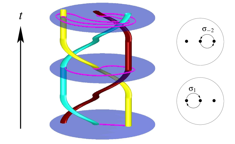
Figure 1: The trajectories of the $N$ stirrers define a braid on $N$ strands in a space-time diagram (here $N=3$), with time flowing from bottom to top. The periodic movement of the stirrers for the protocol is represented in the two pictures on the right: first (bottom) the two rods on the left are interchanged clockwise (we call this operation $\sigma_{1}$), then (top) the two rods on the right are interchanged anti-clockwise ($\sigma_{-2}$). Two sequences of this protocol are drawn on the 3D braid. This protocol is the pseudo-Anosov protocol described in Boyland2000 .

II Braids and Dynamical Systems

II.1 Overview of Thurston–Nielsen (TN) Theory

The mathematical setting for studying braiding in fluids mechanics is centered on the $N$-punctured disk in two dimensions, $R_{N}$. The $N$ punctures, located somewhere in the interior of the disk, represent the stirring rods. If the stirrers undergo a prescribed periodic motion, they return to their initial position at the end of a full cycle. Naturally, the rods have dragged along the fluid, which obeys some as yet unspecified equations (e.g., Stokes, Navier–Stokes, Euler, non-Newtonian equations, assumption of incompressibility, …). The position of fluid elements is thus determined by some function $\Phi(x,t)$. Since the flow is periodic with period $T$, $\Phi(x,T)$ is a map from $R_{N}$ to itself, and we define

$$f:R_{N}\rightarrow R_{N}\,,\qquad f(x)=\Phi(x,T).$$ (1)

For any realizable fluid motion, $f$ will be an orientation-preserving diffeomorphism of $R_{N}$. The map $f$ takes every fluid element to its position after a complete cycle. It is a diffeomorphism because the physical fluid flows we consider are differentiable and have a differentiable inverse. The map $f$ embodies everything about the fluid movement, and it is thus the main object to be studied.

But in some sense $f$ contains too much information: it amounts to a complete solution of the problem, and there are interesting things we can say about the general character of $f$ without necessarily solving for it. We are also interested in knowing what characteristics of the stirrer motion must be reflected in $f$. This is where the concept of an isotopy class comes in: two diffeomorphisms are isotopic if they can be continuously deformed into each other. This is a strong requirement: continuity means that two nearby fluid elements must remain close during the deformation, and so they are not allowed to “go through” a rod during the deformation, otherwise they would cease to be neighbours. In that sense, isotopy is a topological concept, since it is sensitive to obstacles in the domain (the rods). The isotopy class of $f$ is then the set of all diffeomorphisms that are isotopic to $f$. In fact, an entire class can be represented by just one of its members, appropriately called the representative. Of course, the important point here is that that not all diffeomorphisms are isotopic to the identity map. Note that the overwhelming majority of $f$ are not allowable fluid motions (i.e., they cannot arise from the dynamical equations governing the fluid motion), but any allowable fluid motion must belong to some isotopy class.

The problem now is to decide what isotopy classes are possible, and what this means for fluid motion. Thurston–Nielsen (TN) theory Thurston1988 ; Boyland1994 guarantees the existence in the isotopy class of $f$ of a representative map, the TN representative $f^{\prime}$, that belongs to one of three categories:

1. finite-order: if $f^{\prime}$ is repeated enough times, the resulting diffeomorphism is isotopic to the identity (i.e., ${f^{\prime}}^{m}$ is isotopic to the identity for some positive integer $m$);

2. pseudo-Anosov (pA): $f^{\prime}$ stretches fluid elements by a factor $\lambda>1$, so that repeated application gives exponential stretching;

3. reducible: $f^{\prime}$ can be decomposed into components acting on smaller regions of the previous two types.

A famous example of an Anosov map is Arnold’s cat map Arnold . A pA map is an Anosov map with a finite number of singularities. The TN theory also states that the dynamics of a diffeomorphism in a pA isotopy class are at least as complicated as the dynamics of its pA TN representative, meaning it has a greater or equal topological entropy. For a diffeomorphism, the topological entropy $h$ gives a measure of the complexity, i.e. the amount of information which we lose at each iteration of the map Newhouse1993 . It also describes the exponential growth rate of the number of periodic points as a function of their period. Newhouse and Pignataro Newhouse1993 noticed that $h$ also gives the exponential growth rate for the length of a suitably chosen material line. In the numerical simulations described below, we use this fact to compute the topological entropy of a flow: we consider a small blob in the chaotic region of the flow and we calculate the growth rate of its contour length.

TN theory tells us about the possible classes of diffeomorphisms that can arise from the periodic motion of the stirrers. But one can also consider the trajectories of the punctures (here the stirrers) in a 3D space-time plot (Fig. 1), where the vertical is the time axis. These trajectories loop around each other and form a physical braid. The crucial point is that such a braid constructed from the rod trajectories specifies the isotopy class of $f$, no matter the details of the flow. (See Refs. Boyland1994 ; Boyland2000 ; Boyland2003 ; Birman2004 for further details.) As a consequence of the TN theory, the topological entropy of this braid is a lower bound on the topological entropy of the flow.

Hence, determining the isotopy class of the diffeomorphism $f$ is equivalent to studying the braid traced by the stirrer trajectories. This is a drastic reduction in complexity, because we are free to impose relatively simple braiding on the stirrers by means of a short sequence of rods exchanges, whereas the resulting diffeomorphism obtained by solving the fluid equations can be quite complicated. In the next section we introduce the machinery needed to characterize braids.

II.2 Artin’s Braid Group

Let us introduce now the notation for braids. The generators of the Artin braid group on $N$ strands are written $\sigma_{i}$ and $\sigma_{i}^{-1}\mathrel{=\!\!\raisebox{0.29707pt}{:}}\sigma_{-i}$, which represent the interchange of two adjacent strands at position $i$ and $i+1$. The interchange occurs in a clockwise fashion for $\sigma_{i}$ ($i$ goes over $i+1$ along, say, the $y$-axis) and anti-clockwise for $\sigma_{-i}$ ($i$ goes under $i+1$). For $N$ strands, there are $N-1$ generators, so $i\in\{1,\ldots,N-1\}$. It is thus possible to keep track of how $N$ rods are permuted and of the way they cross by writing a braid word with the “letters” $\sigma_{i}$. We read braid words from left to right (that is, in $\sigma_{1}\sigma_{3}\,\sigma_{-2}$ the generator $\sigma_{1}$ precedes $\sigma_{3}$ temporally). For example, the pA stirring protocol described by Boyland et al. Boyland2000 and shown in Fig. 1 corresponds to $\sigma_{1}\sigma_{-2}$: it consists of first interchanging the two rods on the left clockwise ($\sigma_{1}$) and then interchanging the two rods on the right anti-clockwise ($\sigma_{-2}$). Note that the $i$ index on $\sigma_{i}$ refers to the relative position of a rod (e.g., second from the left along the $x$-axis) and does not always label the same rod.

The generators obey the presentation of the braid group,

$$\sigma_{i}\sigma_{j}\sigma_{i} =\sigma_{j}\sigma_{i}\sigma_{j}\qquad \mbox{if}\qquad|i-j| =1,$$ (2a)

$$\sigma_{i}\sigma_{j} =\sigma_{j}\sigma_{i}\qquad \mbox{if}\qquad|i-j| \geq 2,$$ (2b)

that is, the relations (2) must be obeyed by the generators of physical braids, and no other nontrivial relations exist in the group Birman2004 . The relation (2a) corresponds physically to the “sliding” of adjacent crossings past each other, and (2b) to the commutation of nonadjacent crossings.

The braid group on $N$ strands has a simple representation in terms of $(N-1)\times(N-1)$ matrices, called the Burau representation Burau1936 . For three strands ($N=3$), the topological entropy of the braid is obtained from the magnitude of the largest eigenvalue of the Burau matrix representation of the braid word. This is the technique used in Refs. Boyland2000 ; Boyland2003 ; Vikhansky2003 ; Finn2003 to compute topological entropies. For $N>3$ the Burau representation only gives a lower bound on the topological entropy of the braid Kolev2003 , so a more powerful algorithm must be used to obtain accurate values. Here we use the train-tracks code written by T. Hall HallTrain , an implementation of the Bestvina–Handel algorithm Bestvina1995 . The train-tracks algorithm works by computing a graph of the evolution of edges between rods under the braid operations. It suffices for our purposes to say that train-tracks determine the shortest possible length of an “elastic band” that remains hooked to the rods during their motion—the minimum stretching of material lines Finn2005 .

III Evidence for Ghost Rods

III.1 Motivation

We consider here the advection of a passive scalar in a two-dimensional batch stirring device containing a viscous fluid that obeys Stokes’ equation. The batch stirrer includes circular cylinders—the stirring rods—that undergo periodic motion. The exact velocity field for one circular rod in a Stokes flow was derived in Ref. Finn2001 . For more than one rod there is no exact expression available for the velocity field, so we use instead a series expansion suggested by Finn et al. Finn2003 . We use an adaptive fourth-order Runge–Kutta integrator for the time-stepping.

We study first a configuration of the translating rotating mixer (TRM) defined by Finn et al. Finn2001 . The system consists of a two-dimensional disk stirred by a circular rod that moves around in the disk. The center of the rod moves on an epicyclic path (in a time period $T$) given by

$$\begin{split}x(t)&=r_{1}\cos{2\pi mt/T}+r_{2}\cos{2\pi nt/T},\\ y(t)&=r_{1}\sin{2\pi mt/T}+r_{2}\sin{2\pi nt/T},\end{split}$$ (3)

as shown in Fig. 2. Note that such a path can be implemented in a real mixing device using straightforward gearing. It is possible to choose very complicated trajectories by changing $m$ and $n$, however we limit ourselves to the comparatively simple case $m=1$ and $n=2$. The other parameter values used here are $r_{1}=0.2$, $r_{2}=0.5$. The radius of the outer disk is $1$ and we tested configurations with different values for the rod radius $a_{\mathrm{in}}$.

Figure 2: A rod traveling on a epicyclic path. The trajectory of the rod encloses two different regions, a loop and a crescent.

There is only one rod so the one-strand braid formed by the stirrer is trivial. Topologically, the motion of this single rod does not imply a positive lower bound on the topological entropy of the flow. This does not mean that material lines cannot grow exponentially for this flow. We have plotted in Fig. 3 the image of a small blob, i.e. a circle enclosing the rod at $t=0$, after just four periods of the flow with $a_{\mathrm{in}}=0.05$. The small blob has been tremendously stretched, suggesting exponential growth.

Furthermore, note some similarities with another stirring protocol, where the rod is moving on the same path but we have added two fixed rods in the regions enclosed by the moving rod’s trajectory (Fig. 3). For this protocol the braid formed with the stirrers is $\sigma_{-2}\sigma_{-1}\sigma_{-1}\sigma_{-1}\sigma_{-1}\sigma_{-2}$ Finn2003 with topological entropy $h_{\mathrm{braid}}=1.76$. (From now on, we shall use $h_{\mathrm{braid}}$ to denote the topological entropy of a braid, which is a lower bound on the corresponding flow’s topological entropy, $h_{\mathrm{flow}}$: $h_{\mathrm{braid}}\leq h_{\mathrm{flow}}$.) Thus we expect the efficient stretching displayed in Fig. 3. The braid’s entropy is a lower bound for the entropy of the flow, and we indeed measure $h_{\mathrm{flow}}=2.38$. (We recall that we compute $h_{\mathrm{flow}}$ by calculating the exponential rate of growth of material lines in the chaotic region.)

There is thus a discrepancy in that the motion of the rod in Fig. 3 does not account for the observed exponential stretching of material lines, at a rate given by $h_{\mathrm{flow}}=2.32$. An indication of the source of the missing topological entropy is that this rate is comparable to the one observed in the protocol of Fig. 3, $h_{\mathrm{flow}}=2.38$, where extra obstacles are present. We shall see in the following sections that the “missing” topological entropy can be accounted for by looking at periodic orbits in the flow and their topological effect on material lines.

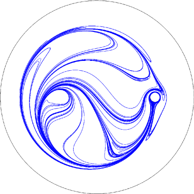
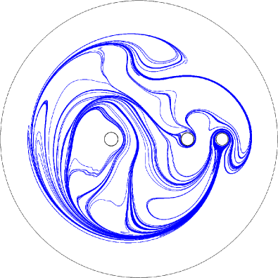
Figure 3: (a) The stretching of a small blob initially surrounding the moving rod; (b) Same as in (a), except two extra fixed rods are inserted in the flow. The patterns made by the blob in (a) and (b) look similar, suggesting that there are invisible topological obstacles in (a) as the fixed rods in (b). Note in particular the similarity between the fixed rod inside the loop in (b) and the way the line wraps itself around an invisible obstacle inside the loop in (a).

III.2 Elliptic Islands as Ghost Rods

In Section III.1 we saw that much of the topological entropy in a one-rod protocol could be accounted for by adding two fixed rods to the flow. These fixed rods modify the flow, but they do not significantly modify the topology of advected material lines compared to the single-rod case (Fig. 3). Hence, for the TRM with only one rod we observe that material lines grow as if rods were present inside the loops traced by the physical rod’s trajectory. This justifies introducing the notion of “ghost rods”: something inside the physical rod’s trajectory is playing the role of a real rod, and we shall soon see that in this case elliptical islands are the culprits. These islands braid with the physical rod, and taken together they give a positive topological entropy. In general, we refer to periodic structures of the flow (islands or isolated points) as ghost rods when they play a role in determining the topological entropy. These are topological obstacles and are thus candidates for forming nontrivial braids. The topological approach puts all periodic structures—orbits and rods—on the same footing.

The introduction of ghost rods becomes even more relevant if one considers the one-rod protocol pictured in Fig. 4. The rod is moving on a figure-eight path, traveling clockwise on the left circle of the eight and anticlockwise on the right circle. A Poincaré section reveals two small islands inside both circles (see Fig. 4). Initial conditions inside these islands remain there forever and are thus topologically equivalent to a fixed rod inside each circle of the figure-eight. By studying the motion of the rod closely, it is easy to show that the braid formed by the rod and the islands is $\sigma_{1}\sigma_{-2}\sigma_{-2}\sigma_{1}$, which has a topological entropy $h_{\mathrm{braid}}=1.76$. Indeed, we measure a topological entropy $h_{\mathrm{flow}}=2.25$, which is greater than $1.76$. (We shall account for the difference with the measured topological entropy of the flow later.) Hence, although elliptic islands are usually considered barriers to mixing, they can also yield a lower bound on the topological entropy of the region exterior to them. All the results presented here for the figure-eight protocol are for the parameters $a=0.35$ (radius of the circles forming the eight), $a_{\mathrm{in}}=0.04$ (radius of the rod) and $a_{\mathrm{out}}=1$ (radius of the outer circle).

So far we have only considered period-1 islands that stay into the regions bounded by the rod’s trajectory, but this is not always possible. In general we have to consider more complicated orbits. For instance, the two islands inside the eight (Fig. 4) are not present for protocols with a larger rod radius $a_{\mathrm{in}}$: in that case we have not found any points that remain forever inside one of the circles. Similarly, for the epicyclic path (Fig. 2) there is an island inside the loop part of the trajectory; however any point will leave the crescent region after a finite time because of the ascending movement induced by the rod, so there are no fixed ghosts rods in that region. The Poincaré section shown in Fig. 5 suggests however other candidates for ghost rods. First, as we noted before, there is a period 1 island that remains inside the loop forever. Second, the Poincaré section reveals three islands that are part of the same period-3 structure. Two “images” of this period-3 island are inside the crescent. The braid formed by the rod and these four islands is shown in Fig. 6.

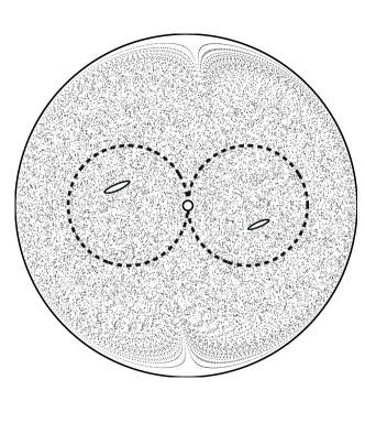
Figure 4: Poincaré section for a protocol with one rod traveling on a figure-eight path (dashed line). Two regular islands are present inside each loop of the rod’s path. They are topological obstacles that form a non-trivial braid with the rod.

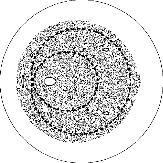
Figure 5: Poincaré section for the TRM protocol, showing different kinds of topological obstacles. The physical rod is moving on an epicyclic path whereas a regular island stays inside the loop and three islands of period three are permuted each period. The braid formed with the rod and these islands is shown in Fig. 6

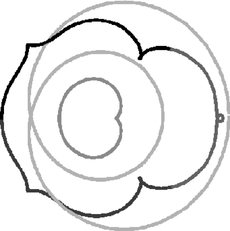
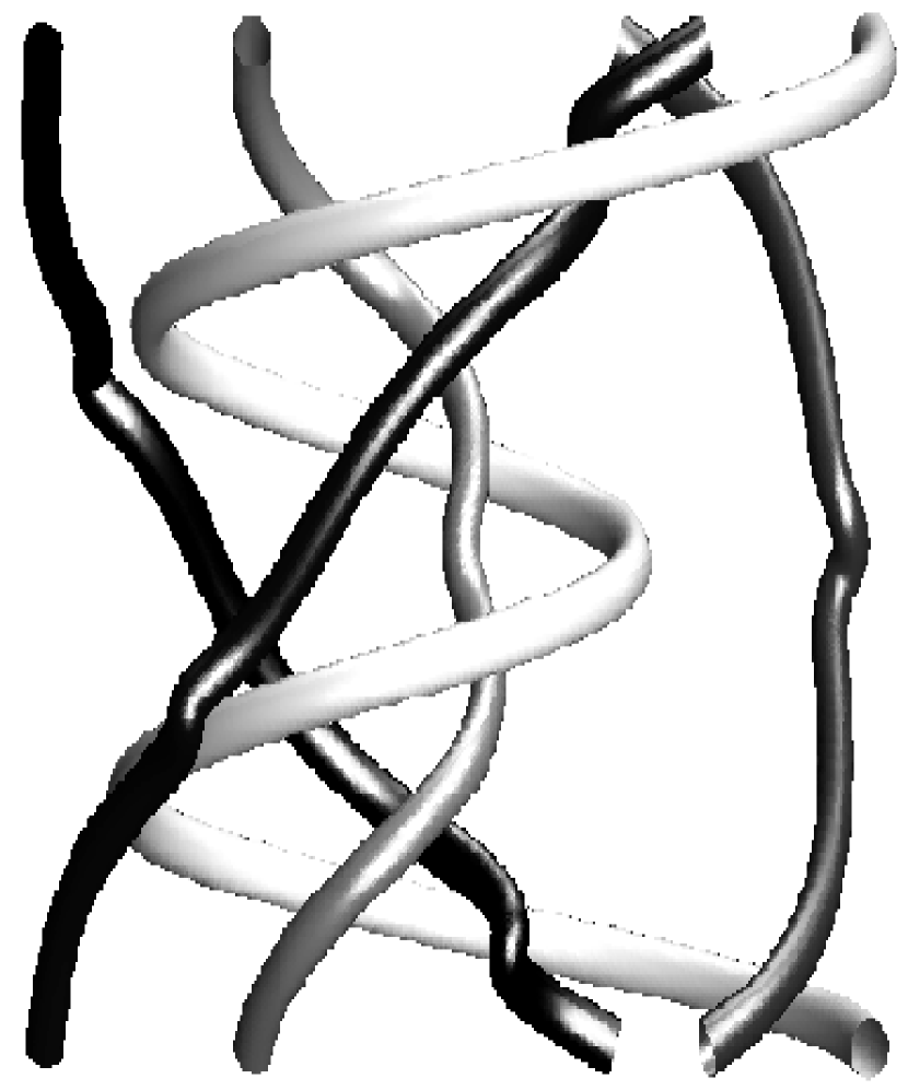
Figure 6: (a) Trajectories of the topological obstacles (the physical rod and two periodic islands) shown in Fig. 5. (b) The same trajectories in a space-time diagram form a braid with positive topological entropy $h_{\mathrm{braid}}=1.72$.

We now have a first method of computing a lower bound on the topological entropy of a flow: look for elliptic islands and calculate the braid formed by the physical rod(s) (if any) and the islands (the ghost rods). Its entropy $h_{\mathrm{braid}}$ will be a lower bound on the topological entropy of the flow $h_{\mathrm{flow}}$. However, this lower bound is often not a very good one: we show in the next section that it is possible to improve it by considering not only islands, but also more general (unstable) periodic orbits.

III.3 Unstable Periodic Orbits as Ghost Rods

A positive topological entropy implies a horseshoe structure Katok1980 and thus an infinite number of unstable periodic orbits (UPO’s) in the flow. These periodic points are topological obstacles as well as the physical rods (though they have zero size), and hence are ghost rods. However, most periodic points are unstable and therefore difficult to detect: a trajectory initialized near an unstable periodic point will diverge from the periodic orbit (exponentially for a hyperbolic orbit). We use the method of Schmelcher and Diakonos Schmelcher1998 to detect periodic orbits numerically. The method relies on finding the periodic orbits of a modified version of the flow that has the same periodic orbits, except that they are stable in the modified flow. Diakonos et al. Diakonos1998 point out that this method selects the least unstable orbits, that is, the least unstable orbits are found first and one has to change a parameter in the algorithm and therefore increase the computing time to find more unstable orbits. Furthermore, we are dealing with systems with high topological entropy: as asymptotically the flow has roughly $\exp{(h_{\mathrm{flow}}n)}$ periodic points of period $n$, systematic detection of periodic points is impossible for orbits of high order. We choose rather to detect only the least unstable orbits: we show in the next section that it is possible to derive an accurate value of the topological entropy of a flow from these orbits.

IV Calculating the Topological Entropy with Ghost Rods

Boyland Boyland1994 , using results by Katok Katok1980 , proved that for an orientation-preserving diffeomorphism of the disk there exists a sequence of orbits whose entropies converge to the topological entropy of the flow. The topological entropy can thus be obtained from the periodic-orbit structure of the flow. It should therefore be possible to find a periodic orbit whose braid has a topological entropy arbitrarily close to the topological entropy of the flow. We investigate this before considering multiple periodic orbits.

A periodic orbit is self-braiding if the points in the orbit form a nontrivial braid when taken together. Figure 7 shows

Figure 7: (a) Some periodic orbits are self-braiding, that is, the entropy of the braid formed by all the points of the orbit is strictly positive. The entropy of the self-braiding orbits is plotted here vs their period. (b) The positive entropy of braids formed by the rod’s trajectory and pairs of periodic orbits vs the number of strands in the braid. In both plots, the solid line is the measured topological entropy of the flow, $h_{\mathrm{flow}}=2.25$.

the topological entropy of self-braiding orbits as a function of their period for the figure-eight protocol. Some orbits indeed have a positive topological entropy, but their entropy is far from the one computed with the line-growth algorithm ($h_{\mathrm{flow}}=2.25$), solid horizontal line in Fig. 7. Furthermore very few orbits self-braid, i.e. have a positive entropy. Hence, it appears that looking at the topological entropy of individual orbits is not very useful: obtaining a reasonable approximation to the topological entropy requires orbits of prohibitively high order or instability.

As self-braiding orbits do not seem very convenient to approach $h_{\mathrm{flow}}$ we choose rather to combine several orbits together to form more complex braids. We first combine each periodic orbit with the rod and we obtain higher values for $h_{\mathrm{braid}}$, although still far from $h_{\mathrm{flow}}$. We also consider the braids formed by the rod and pairs of periodic orbits, which are also invariant sets of the first return map. We consider pairs of orbits because this is the minimal number of orbits that can capture the topology determined by the rod’s trajectory. As is shown in Fig. 7, we obtain braid entropies far closer to the value measured for the flow: some braids approximate the measured entropy to within numerical error. It is thus more efficient to consider combinations of orbits rather than only self-braiding orbits: one would surely need orbits of very high order, or very unstable, to get as close to the measured value $h_{\mathrm{flow}}$. For this example we used a set of $52$ periodic orbits whose positive Floquet exponent is smaller than $3/T$, where $T$ is the period of the orbit. Note that although we did not detect all or even a large number of periodic orbits (there is an infinity of them), our combination of ghost rods provides us with a very good approximation of the topological entropy of the flow. For a given system the entropy lower bound must increase as more orbits are added to a given braid; nevertheless we see that for the system we consider, only a small number of orbits is needed to obtain a satisfactory lower bound on $h_{\mathrm{flow}}$. We therefore suggest an alternative method for calculating the topological entropy of a flow: (i) detect some periodic orbits; (ii) calculate the maximum entropy of all the braids one can create with these points and the rod(s); and (iii) see if this maximum entropy converges when one increases the number of periodic orbits.

V Discussion

To summarize, we have characterized chaos in two-dimensional time-periodic flows by considering the braids formed by periodic points and calculating their topological entropy for different stirring protocols. We have demonstrated the role of periodic points in fluid mixing, and called these periodic points ghost rods because their movement stretches material lines as real stirring rods do. This work is an extension of the topological kinematics theory introduced by Boyland et al. Boyland1994 ; Boyland2000 ; Boyland2003 , since it characterizes the mixing in a flow by studying the topological constraint induced by the ghost rods and not only stirrers. We expect this approach to develop further in the near future, and to yield new insight on efficient mixing devices.

The idea of characterizing dynamics of homeomorphisms of surfaces by puncturing at periodic orbits dates back to Bowen Bowen1978 , and the study of braids formed with periodic points had already been suggested by Boyland for the general study of diffeomorphisms of the disk Boyland1994 . In addition, this technique is used in other fields such as the study of optical parametric oscillators Amon2004 . However, the present work is to our knowledge the first study of ghost rods in fluid mechanics.

In contrast to other applications, in our systems the ghost rods are created by the movement of the physical rod, so we may hope to derive some information about ghost rods from the motion of that physical rod. For instance, let us consider the period-3 orbit for the figure-eight protocol shown in Fig. 8

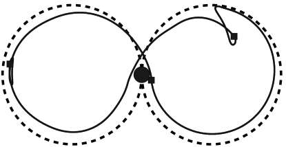
Figure 8: The trajectory of the rod (dashed line) and three period-3 points belonging to the same orbit (solid line). The position of the rod (filled circle) and the periodic points (filled squares) at $t=0$ is also shown.

(this orbit is more unstable than the ones we used in the previous section). One point of the orbit is located very close to the physical rod at $t=0$. Its trajectory will thus be very close to the rod’s trajectory at the beginning of the period. Later the rod leaves the periodic point in its trail after a time equal to about $T/3$. One period later the rod drags this point again on its trajectory as it comes close to it. This accounts for the topological similarity between the trajectory of the rod and the periodic orbit. The braid formed by these period-3 orbits is $\sigma_{-1}\sigma_{2}$, which is also the braid studied by Boyland et al. in Boyland2000 . It is actually the braid with the maximal $h_{\mathrm{braid}}$ that we can form with points moving on a trajectory strictly equivalent to the rod’s path. Indeed we cannot form a braid with fewer than three points, and periodic points with a higher period on such a path move slower as they take longer to cover the whole path, so they have a less efficient braiding (fewer exchanges per period). We conjecture that this type of figure-eight trajectory is characteristic of all mixing protocols with a rod moving on a figure-eight path.

We have indeed found such a braid—formed by a period-3 orbit equivalent to the rod’s trajectory—for all the figure-eight protocols we have tested. We have tried the protocol plotted in Fig. 4 with different radii for the rod, as well as a protocol with one rod moving on a lemniscate (a lemniscate is the more natural “figure-eight” shape lemniscate ), and we have detected this figure-eight periodic orbit associated with the $\sigma_{-1}\sigma_{2}$ braid for each protocol. It is thus very tempting to conjecture that for all the Stokes flows created by the movement of a rod on a figure-eight path, the topological entropy of the flow is greater than the entropy of the braid $\sigma_{-1}\sigma_{2}$, that is, $0.96$. If this conjecture holds, then ghost rods can be used not only for diagnosing chaos and calculating the entropy of a flow, but also topological arguments can be used to predict a minimum entropy just from the path of the physical rod with ghost rods in its trail. This is a generalization to ghost rods of the arguments used by Boyland et al. Boyland2000 to predict a universal minimum entropy from the movements of the rods for three or more physical rods. A further natural question then is which ghost rods have the best braid, that is, the braid giving the topological entropy of the flow, and could we relate these “most efficient” ghost rods to the physical properties of the flow? This will be the topic of future research.

The ghost rods approach should also be compared with recent work on nonperiodic points. Thiffeault Thiffeault2005 noticed that every fluid particle in a two-dimensional flow is a topological obstacle, much like a stirrer, and calculated entropies of braids formed by arbitrary chaotic orbits. As these points were not periodic points these entropies may not give a lower bound on the entropy of the flow for short times; however, they can yield finite-time information about the stretching rate of material lines. Furthermore, if one considers long time series, a randomly chosen point in an ergodic chaotic region will repeatedly come very close to periodic orbits. It should thus be possible to observe braids with similar properties as the ones formed by ghost rods.

Finally, the study of ghost rods can be used to prove that a map is chaotic in the case where some periodic points can be calculated analytically, as for the sine flow map Liu1994a ; Finn2005 or the closely-related standard map Chirikov1996 . Finn et al. Finn2005 , for example, have shown that the sine flow map has chaotic trajectories for some parameter values.

References

- (1) H. Aref, “Stirring by chaotic advection,” J. Fluid Mech. 143, 1 (1984).
- (2) J. M. Ottino, The kinematics of mixing: stretching, chaos, and transport (Cambridge University Press, Cambridge, U.K., 1989).
- (3) H. Aref, “The development of chaotic advection,” Phys. Fluids 14, 1315 (2002).
- (4) J. Chaiken, R. Chevray, M. Tabor, and Q. M. Tan, “Experimental study of Lagrangian turbulence in a Stokes flow,” Proc. R. Soc. Lond. A 408, 165 (1986).
- (5) P. L. Boyland, H. Aref, and M. A. Stremler, “Topological fluid mechanics of stirring,” J. Fluid Mech. 403, 277 (2000).
- (6) W. Thurston, “On the geometry and dynamics of diffeomorphisms of surfaces,” Bull. Am. Math. Soc. 19, 417 (1988).
- (7) P. Boyland, “Topological methods in surface dynamics,” Topology Appl. 58, 223 (1994).
- (8) S. Newhouse and T. Pignataro, “On the estimation of topological entropy,” J. Stat. Phys. 72, 1331 (1993).
- (9) P. Boyland, M. Stremler, and H. Aref, “Topological fluid mechanics of point vortex motions,” Physica D 175, 69 (2003).
- (10) J.-L. Thiffeault, “Measuring topological chaos,” Phys. Rev. Lett. 94, 84502 (2005).
- (11) D. Auerbach, P. Cvitanović, J.-P. Eckmann, G. Gunaratne, and I. Procaccia, “Exploring chaotic motion through periodic orbits,” Phys. Rev. Lett. 58, 2387 (1987).
- (12) P. Cvitanović, “Invariant measurement of strange sets in terms of cycles,” Phys. Rev. Lett. 61, 2729 (1988).
- (13) V. I. Arnold, Mathematical Methods of Classical Mechanics, 2nd ed. (Springer-Verlag, New York, 1989).
- (14) J. S. Birman and T. E. Brendle, in Handbook of Knot Theory, edited by W. Menasco and M. Thistlethwaite (Elsevier, Amsterdam, 2005).
- (15) W. Burau, “Über Zopfgruppen und gleichsinnig verdrilte Verkettungen,” Abh. Math. Sem. Hanischen Univ. 11, 171 (1936).
- (16) A. Vikhansky, “Chaotic advection of finite-size bodies in a cavity flow,” Phys. Fluids 15, 1830 (2003).
- (17) M. Finn, S. Cox, and H. Byrne, “Topological chaos in inviscid and viscous mixers,” J. Fluid Mech. 493, 345 (2003).
- (18) B. Kolev, “Entropie topologique et représentation de Burau,” C. R. Acad. Sci. Sér. I 309, 835 (1989).
- (19) T. Hall, Train: A C++ program for computing train tracks of surface homeomorphisms, http://www.liv.ac.uk/maths/PURE/MIN_SET/CONTENT/members/T_Hall.html.
- (20) M. Bestvina and M. Handel, “Train-tracks for surface homeomorphisms,” Topology 34, 109 (1995).
- (21) M. D. Finn, J.-L. Thiffeault, and E. Gouillart, “Topological chaos in spatially periodic mixers,” arXiv:nlin.CD/0507023.
- (22) M. D. Finn and S. M. Cox, “Stokes flow in a mixer with changing geometry,” J. Eng. Math. 41, 75 (2001).
- (23) A. Katok, “Lyapunov exponents, entropy and periodic orbits for diffeomorphisms,” Inst. Hautes Etudes Sci. Publ. Math. 51, 137 (1980).
- (24) P. Schmelcher and F. K. Diakonos, “General approach to the localization of unstable periodic orbits in chaotic dynamical systems,” Phys. Rev. E 57, 2739 (1998).
- (25) F. K. Diakonos, P. Schmelcher, and O. Biham, “Systematic computation of the least unstable periodic orbits in chaotic attractors,” Phys. Rev. Lett. 81, 4349 (1998).
- (26) A. Amon and M. Lefranc, “Topological signature of deterministic chaos in short nonstationary signals from an optical parametric oscillator,” Phys. Rev. Lett. 92, 094101 (2004).
- (27) E. W. Weisstein, Lemniscate, from MathWorld—A Wolfram Web Resource. http://mathworld.wolfram.com/Lemniscate.html.
- (28) M. Liu, F. J. Muzzio, and R. Peskin, “Quantification of mixing in aperiodic chaotic flows,” Chaos Solitons Fractals 4, 869 (1994).
- (29) B. Chirikov, “Anomalous diffusion in a microtron and critical structure at the chaos boundary,” JETP 83, 646 (1996).
- (30) R. Bowen, “Entropy and the fundamental group,” in Structure of Attractors, Lecture Notes in Math. 668, pp. 21–29 (Springer, New York, 1978).