Strange Nonchaotic Attractors in Harper Maps

Abstract

We study the existence of Strange Nonchaotic Attractors (SNA) in the family of Harper maps, proving that they are typical but not robust in this family. Our approach is based on the theory of linear skew-products and the spectral theory of Schrödinger operators.

The study of the attractors of a dissipative dynamical system is a topic of great interest, because these invariant sets trap the evolution of a large subset of the phase space and capture the asymptotic behavior. It has been known for a long time that attractors can be strange Ruelle and Takens (1971), i.e. geometrically complicated. The first examples of strange attractors were chaotic, i.e. with dependence sensitive on initial conditions Eckmann and Ruelle (1985). In Grebogi et al. (1984) were found strange attractors that are nonchaotic, and it has stimulated much numerical experimentation (see the review Prasad et al. (2001)) as well as rigorous analysis Keller (1996); Glendinning (2002); Stark (2003).

Our interest in this Letter is to show the existence and abundance of Strange Nonchaotic Attractors (SNA for short) in the family of Harper maps. This is a family of 1D quasi-periodically forced maps that many authors have suggested as a scenario in which SNA appear Ketoja and Satija (1997, 1995); Prasad et al. (1999); Singh and Ramaswamy (2001); Mestel et al. (2000)Bondeson et al. (1985). By SNA we mean here an invariant set that is a graph of a measurable and nowhere continuous function (it is Strange), that carries a quasi-periodic dynamics (it is Nonchaotic) and it attracts exponentially fast almost every orbit in phase space (it is an Attractor) . We prove that these SNA are typical but not robust in the family of Harper maps, in the sense that they exist for a positive measure Cantor set of the parameter space.

In our analysis, we exploit the connections between (a) the dynamical properties of the Harper map (a 1D quasi-periodically forced map); (b) the spectral properties of the Harper operator (an example of a quasi-periodic Schrödinger operator); (c) the geometrical properties of the Harper linear skew-product (a 2D quasi-periodically forced linear map).

In recent years our knowledge of the spectral properties of the Harper operator, also known as the Almost Mathieu operator, and related quasi-periodic Schrödinger operators has advanced spectacularly. The progress made will be relevant to our approach. In particular, the connections between (b) and (c) have been successfully applied to the solution of the “Ten Martini Problem” Puig (2004), on the Cantor structure of the spectrum of the Harper operator.

The connection between (a) and (c) in similar models has been used to study the linearized dynamics around invariant tori in quasi-periodic systems Haro and de la Llave (2005a). Specifically, the formation of SNA in this linearized dynamics is suggested to be a mechanism of breakdown of invariant tori Haro and de la Llave (2005b).

A consequence of our approach is that neither arithmetic properties of the frequency of the quasi-periodic forcing nor localization properties of the spectrum of the Harper operator are crucial for the existence of SNA.

The family of quasi-periodically forced dynamical systems under investigation in this Letter is the family of Harper maps

$$\begin{array}[]{ccl}y_{n+1}&=&\underbrace{\frac{1}{a-b\cos{(2\pi\theta_{n})}-{y_{n}}}}_{f_{a,b}({y_{n}},\theta_{n})},\\ \theta_{n+1}&=&\theta_{n}+\omega\qquad(\mathrm{mod\leavevmode\nobreak\ }1),\end{array}$$ (1)

where $y\in\overline{\mathbb{R}}=[-\infty,+\infty]$ and $\theta\in\mathbb{T}={\mathbb{R}}/{\mathbb{Z}}$ are the phase space variables, $a,b$ are the parameters, and $\omega$ is the frequency (it is assumed to be irrational).

Notice that a Harper map is a skew-product map

$$F_{a,b,\omega}(y_{n},\theta_{n})=(f_{a,b}(y_{n},\theta_{n}),\theta_{n}+\omega),$$

defining a dynamical system in $\overline{\mathbb{R}}\times\mathbb{T}$ whose evolution from an initial condition $(y_{0},\theta_{0})$ is described by the $Nth$-power $F^{(N)}_{{a,b,\omega}}(y_{0},\theta_{0})=(f^{(N)}_{a,b}(y_{0},\theta_{0}),\theta_{0}+N\omega)$, for $N\in\mathbb{Z}$.

In a Harper map the parameter $a$ is called the energy or the spectral parameter because after writing ${y}_{n}=x_{n-1}/x_{n}$ this family is equivalent to the family of Harper equations, which are second-order difference equations

$$x_{n+1}+x_{n-1}+b\cos\left(2\pi(\theta_{0}+n\omega)\right)x_{n}=ax_{n}.$$ (2)

These equations are physically relevant because they show up as eigenvalue equations of Harper operators (also known as Almost Mathieu operators),

$$\left(H_{b,\omega,\theta_{0}}x\right)_{n}=x_{n+1}+x_{n-1}+b\cos\left(2\pi(\theta_{0}+n\omega)\right)x_{n}.$$ (3)

These are bounded and self-adjoint operators on $l^{2}(\mathbb{Z})$ whose spectrum, that does not depend on $\theta_{0}$, describes the energy spectrum of an electron in a rectangular lattice subject to a perpendicular magnetic flux Harper (1955); Sokoloff (1985).

The formulation of the second-order difference equation (2) as a first-order system is the Harper linear skew-product

$$\begin{array}[]{ccl}\underbrace{\left(\begin{array}[]{c}x_{n+1}\\ x_{n}\end{array}\right)}_{v_{n+1}}&=&\underbrace{\left(\begin{array}[]{cc}a-b\cos\left(2\pi\theta_{n}\right)&\;-1\\ 1&\;\phantom{-}0\end{array}\right)}_{M_{a,b}(\theta_{n})}\underbrace{\left(\begin{array}[]{c}x_{n}\\ x_{n-1}\end{array}\right)}_{v_{n}},\\ \theta_{n+1}&=&\theta_{n}+\omega\qquad(\mathrm{mod\leavevmode\nobreak\ }1),\end{array}$$ (4)

whose evolution is given by the Harper cocycle

$$M^{(N)}_{a,b,\omega}(\theta_{0})=\begin{cases}M_{a,b}\left(\theta_{N-1}\right)\dots M_{a,b}(\theta_{0})&\text{if $N>0$,}\\ I&\text{if $N=0$,}\\ M_{a,b}^{-1}\left(\theta_{N}\right)\dots M_{a,b}^{-1}(\theta_{-1})&\text{if $N<0$.}\end{cases}$$ (5)

Note that (1) describes the evolution of the slope $y_{n}$ of vectors $v_{n}$ under the action of the linear skew-product (4). That is, (1) is the projectivization of (4).

To understand the dynamics of Harper linear skew-products it is important to know the growth properties of the solutions. The exponential growth is measured by the Lyapunov exponents which we now define. Given any nontrivial initial condition of the skew-product (4), $(v_{0},\theta_{0})$ with $v_{0}\neq 0$, the (forward) Lyapunov exponent for $(v_{0},\theta_{0})$ is the limit

$$\begin{split}\lambda_{a,b,\omega}(v_{0},\theta_{0})&=\lim_{N\to+\infty}\frac{1}{N}\log{\left|v_{N}\right|},\\ &=\lim_{N\to+\infty}\frac{1}{N}\log{\left|M_{a,b,\omega}^{(N)}(\theta_{0})v_{0}\right|}\end{split}$$ (6)

whenever the limit exists (in which case it is finite). If $v_{0}=(x_{-1},x_{0})$ and ${y}_{0}=x_{-1}/x_{0}$ then one can also define the (forward) Lyapunov exponent of the Harper map (1) for the initial condition $({y}_{0},\theta_{0})$ by

$$\begin{split}{\beta}_{a,b,\omega}({y}_{0},\theta_{0})&=\lim_{N\to+\infty}\frac{1}{N}\log{\left|\frac{\partial{y}_{N}}{\partial{y}_{0}}({y}_{0},\theta_{0})\right|}\\ &=\lim_{N\to+\infty}\frac{1}{N}\log{\left|m^{(N)}_{a,b,\omega}(y_{0},\theta_{0})\right|}\end{split}$$ (7)

where

$$m^{(N)}_{a,b,\omega}(y_{0},\theta_{0})=\frac{\partial f_{a,b}}{\partial{y}}\left({y}_{N-1},\theta_{N-1}\right)\dots\frac{\partial f_{a,b}}{\partial{y}}\left({y}_{0},\theta_{0}\right)\ .$$

An easy computation shows the relation

$$\beta_{a,b,\omega}({y}_{0},\theta_{0})=-2{\lambda}_{a,b,\omega}(v_{0},\theta_{0}).$$

Backward Lyapunov exponents are defined by replacing $\lim_{N\to+\infty}$ with $\lim_{N\to-\infty}$ in the above formulation.

Oseledec Oseledec (1968) showed that for almost every initial condition $(v_{0},\theta_{0})$ the Lyapunov exponent exists and equals the averaged Lyapunov exponent

$$\overline{\lambda}_{a,b,\omega}=\lim_{N\to+\infty}\frac{1}{N}\int_{\mathbb{T}}\log{\left|M^{(N)}_{a,b,\omega}(\theta)\right|}d\theta,$$

which is never negative and exists by the Kingman subadditive ergodic theorem Kingman (1968).

The case of the nonzero averaged Lyapunov exponent, $\overline{\lambda}_{a,b,\omega}>0$, which we call hyperbolic, is important for our purposes. In this case, there exists a full measure set $\Theta\subset\mathbb{T}$ such that for every $\theta\in\Theta$ one has a splitting

$$\mathbb{R}^{2}=W^{s}(\theta)\oplus W^{u}(\theta)$$ (8)

characterized by

$$v\in W^{s}(\theta)\setminus\{0\}\quad\Leftrightarrow\quad\lim_{N\to\pm\infty}\frac{1}{N}\log{\left|M^{(N)}(\theta)v\right|}=-\overline{\lambda}$$ (9)

and

$$v\in W^{u}(\theta)\setminus\{0\}\quad\Leftrightarrow\quad\lim_{N\to\pm\infty}\frac{1}{N}\log{\left|M^{(N)}(\theta)v\right|}=+\overline{\lambda}.$$ (10)

$W^{s}(\theta)$ and $W^{u}(\theta)$ are the stable and unstable subspaces at $\theta$, respectively. The elements of the set $\Theta$ are referred to as the Lyapunov regular points.

In the phase space $\mathbb{R}^{2}\times\mathbb{T}$, one can form the product sets $W^{s}$ and $W^{u}$ whose elements are pairs $(v,\theta)$ with $v\in W^{s}(\theta)$ or $W^{u}(\theta)$ respectively (whenever these subspaces are defined). These are the stable and unstable subbundles. According to Oseledec Oseledec (1968) the $\theta$-dependence of the decomposition is measurable but not necessarily continuous.

When the splitting (8) is defined for all $\theta$, that is $\Theta=\mathbb{T}$ (hence $\theta$-dependence of the subbundles is continuous ) the linear skew-product is said to be uniformly hyperbolic. Otherwise it is said to be nonuniformly hyperbolic.

In the Harper map, we can determine whether or not hyperbolicity is uniform by looking at the spectral problem of (3). Indeed, an energy $a$ is in the spectrum of the Harper operator (3) if, and only if, the corresponding linear skew-product (4) is not uniformly hyperbolic Mañé (1978); Johnson (1982). We will use an implication of this result: if $a$ is in the spectrum of the Harper operator and the averaged Lyapunov exponent is nonzero at $a,$ then the linear skew-product is nonuniformly hyperbolic. Let us now see that in this case the corresponding Harper map has a SNA.

The above concepts of hyperbolicity can be translated to the dynamics of the Harper map (1) (which reflects how the linear skew-product (4) changes directions of vectors). Recall that, in the hyperbolic case, ${\beta}<0$, there exist two invariant subbundles $W^{s}$ and $W^{u}$, for $\theta\in\Theta$, which are measurable as a function of $\theta$ and satisfy (9) and (10). We define ${y}^{s}(\theta)$ and ${y}^{u}(\theta)$ as the slopes of the subbundles: they are the only elements of ${\overline{\mathbb{R}}}$ such that $(1,{y}^{s}(\theta))^{T}$ and $(1,{y}^{u}(\theta))^{T}$ belong to $W^{s}(\theta)$ and $W^{u}(\theta)$ respectively. The product sets

$$Y^{s}=\left\{({y}^{s}(\theta),\theta),\;\theta\in\Theta\right\}\text{ and }Y^{u}=\left\{({y}^{u}(\theta),\theta),\;\theta\in\Theta\right\}$$

are invariant under the Harper map and have quasi-periodic dynamics; thus ${Y}^{s}$ and ${Y}^{u}$ are nonchaotic invariant sets.

Still in the hyperbolic case, the decomposition of $\mathbb{R}^{2}$ into direct sum of $W^{s}(\theta)$ and $W^{u}(\theta)$, $\theta\in\Theta$, implies that every pair $(v,\theta)$ of this skew-product (4) other than the stable subbundle, is attracted to the unstable subbundle and grows exponentially in norm. Looking at directions (which is what the Harper map retains), forward orbits with initial condition $({y},\theta)$ (other than $({y}^{s}(\theta),\theta)$) are exponentially attracted to ${Y}^{u}$, that is

$$\lim_{N\to+\infty}\frac{1}{N}\log\left|f_{a,b,\omega}^{(N)}({y},\theta)-{y}^{u}(\theta_{N})\right|=\beta=-2\overline{\lambda}<0,$$ (11)

while backward orbits (other than $({y}^{u}(\theta),\theta)$) are exponentially attracted to ${Y}^{s}$. Thus ${Y}^{u}$ is a nonchaotic attractor for the Harper map: for almost every initial condition, orbits are exponentially attracted to it. Similarly $Y^{s}$ is a nonchaotic repellor.

Let us now relate the uniformity of hyperbolicity in the skew-product to the regularity of these nonchaotic attractors. If the skew-product (4) is uniformly hyperbolic then the invariant subbundles $W^{s}$, $W^{u}$ are defined in all $\mathbb{T}$ and are continuous, and so are their projectivizations ${y}^{u}$ and ${y}^{s}$.

In contrast, if the skew-product is nonuniformly hyperbolic, then the invariant subbundles are measurable but not continuous and their projectivizations ${y}^{u}$ and ${y}^{s}$ are measurable but not continuous functions of $\theta$. Moreover, discontinuities are propagated by the quasi-periodic dynamics and the invariance property of the attractor: if ${y}^{u}$ is discontinuous at a single $\theta_{0}$ then the same happens for $\theta_{N}=\theta_{0}+N\omega$ for all $N\in\mathbb{Z}$, so that the function ${y}^{u}$ is nowhere continuous. The same result happens for ${y}^{s}$.

In summary, in the nonuniformly hyperbolic case, we will say that $Y^{u}$ is a Strange Nonchaotic Attractor (SNA) of the Harper map because the following properties are satisfied:

1. $Y^{u}$ is the graph of a measurable function of $\theta$, $y^{u}$, which is nowhere continuous ($Y^{u}$ is Strange);

2. $Y^{u}$ is an invariant set of the Harper map with quasi-periodic dynamics ($Y^{u}$ is Nonchaotic);

3. Almost every orbit in phase space is attracted to ${Y}^{u}$ at exponential rate ($Y^{u}$ is an Attractor).

The existence of nonuniformly hyperbolic linear skew-products was already shown by Herman Herman (1983), who proved that

$$\overline{\lambda}_{a,b,\omega}\geq\max\left(0,\log\frac{|b|}{2}\right)$$ (12)

as long as $\omega$ is irrational. Moreover, Bourgain & Jitomirskaya Bourgain and Jitomirskaya (2002) prove that the equality in (12) holds if, and only if, $a$ is in the spectrum of the Almost Mathieu operator.

Thus, for $|b|>2$ and $\omega$ irrational, a Harper map has a SNA if, and only if, $a$ belongs to the spectrum. Since the measure of the spectrum is given by the formula $|4-2|b||$ Jitomirskaya and Krasovsky (2002) these SNA are persistent in measure in the family of Harper maps. They are not, however, persistent in open sets, since the spectrum is a Cantor set Choi et al. (1990); Puig (2004); Avila and Jitomirskaya (2005), and therefore any SNA in a Harper map can become a regular attractor by means of an arbitrarily small perturbation. As an example, using the symmetry of the spectrum, the Harper map has a SNA for any $|b|>2$, $\omega$ irrational and $a=0$ (this value always belongs to the spectrum).

As an illustration of the above rigorous results, we performed several numerical computations. In the following, we chose the irrational frequency $\omega=\displaystyle\frac{e}{4}$ , $b=3$, and we considered $a$ as a moving parameter. The averaged Lyapunov exponent as a function of $a$ is displayed in Figure 1. Notice that (12) implies that $\overline{\lambda}_{a}\geq\frac{\log 3}{2}$, so that the Harper cocycle is hyperbolic for all the values $a$. Moreover, the equality holds only if the cocycle is nonuniformly hyperbolic. As a result, the values of $a$ for which $Y^{u}$ is a SNA of the Harper map correspond to the “flat pieces” of the graph in Figure 1, which lie in a Cantor set of measure 2. The “bumps” appear in gaps of the spectrum, that is energies $a$ in the resolvent set, for which $Y^{u}$ is an invariant attracting continuous curve. Hence, gaps are labelled by a topological index which is the number of turns of $Y^{u}$ on $\overline{\mathbb{R}}$ Johnson and Moser (1982).

We also selected several values of $a$ and computed the attractor $Y^{u}$ and the repellor $Y^{s}$ of the Harper map for several values of $a.$ The results are displayed in Figures 2 and 3. Since $y\in{\overline{\mathbb{R}}}$ represents a slope, in the pictures we display the angle $\varphi=\tan^{-1}y\in[-\pi/2,\pi/2]$ corresponding to such a slope. In this representation we identify $\varphi=\pi/2$ with $\varphi=-\pi/2$, because a line of slope $+\infty$ is a line with slope $-\infty$. The objects shown are graphs of functions $y^{u}(\theta)$, $y^{s}(\theta)$, respectively, of the slope $y\in{\overline{\mathbb{R}}}$ with respect to $\theta$.

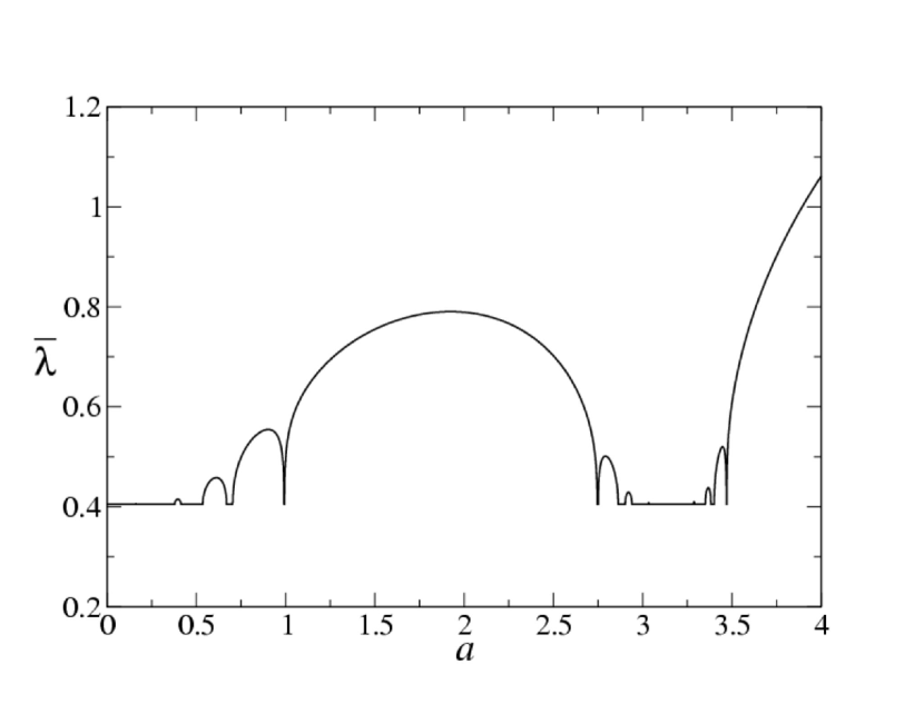
Figure 1: The averaged Lyapunov exponent as a function of $a$.

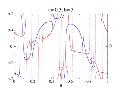
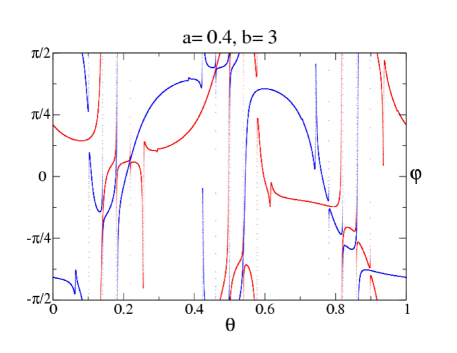
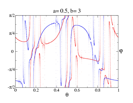
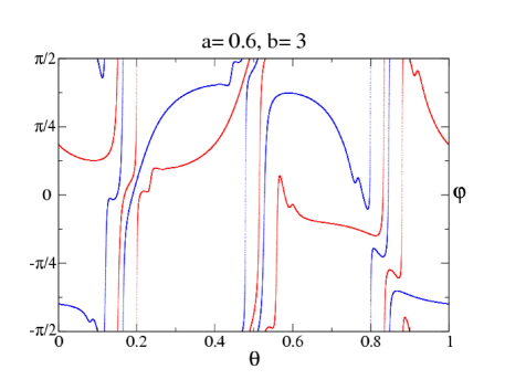
Figure 2: The attractor $Y^{u}$ and the repellor $Y^{s}$ of the Harper map for $a=0.3,0.5$ (SNA) and $a=0.4,0.6$ (continuous invariant curves). Notice that $a=0.4$ and $a=0.6$ correspond to different gaps which are labelled by the indices of the continuous curves $8$ and $5$, respectively.

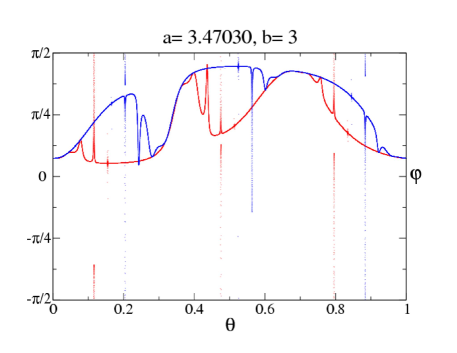
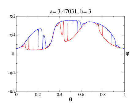
Figure 3: The attractor $Y^{u}$ and the repellor $Y^{s}$ of the Harper map for $a=3.47030$ (SNA) and $a=3.47031$ (continuous invariant curves). Notice the dramatic change in the dynamics with a very small perturbation of $a$. The value $a=3.47031$ belongs to the rightmost gap, whose index is $0$ (see Figure 1).

In this Letter we have shown the existence of SNA in Harper maps with $\omega$ irrational, $|b|>2$ and $a$ in the spectrum without resorting to the possible localization properties of the spectral problem. Recall that $a$ is a point eigenvalue of a Harper operator $H_{b,\omega,\theta_{0}}$ if the corresponding eigenvalue (Harper) equation has a nontrivial localized solution $\psi=(\psi_{n})_{n\in\mathbb{Z}}$ which is square integrable or even decays exponentially with $|n|$. If the set of localized eigenvectors of a Harper operator forms a complete orthogonal basis of $l^{2}(\mathbb{Z})$ then the spectrum is pure-point.

In previous work on the existence of SNA in Harper maps, localization was seen as a justification for the strangeness of SNA, in the regime of nonzero Lyapunov exponents Ketoja and Satija (1997, 1995); Mestel et al. (2000); Mestel and Osbaldestin (2004a, b). As we have seen, we do not use localization to prove the existence of SNA. Besides, localization may not hold in all the Harper maps studied here. Indeed, an energy $a$ in the spectrum of a Harper operator with nonzero Lyapunov exponent (for which the Harper map has an SNA) may not be an eigenvalue of the operator. Indeed, if $\omega$ is not Diophantine, localization may only hold for $|b|>2$ large enough (depending on $\omega$) Avila and Jitomirskaya (2005). Even in the Diophantine case, the spectrum also contains a residual set of energies which are not point eigenvalues Jitomirskaya and Simon (1994); Puig (2005). Thus, there are SNA in the family of Harper maps without localization for the corresponding operator or arithmetic properties on $\omega$.

References

- Ruelle and Takens (1971) D. Ruelle and F. Takens, Comm. Math. Phys. 20, 167 (1971).
- Eckmann and Ruelle (1985) J.-P. Eckmann and D. Ruelle, Rev. Modern Phys. 57, 617 (1985).
- Grebogi et al. (1984) C. Grebogi, E. Ott, S. Pelikan, and J. A. Yorke, Phys. D 13, 261 (1984).
- Prasad et al. (2001) A. Prasad, S. S. Negi, and R. Ramaswamy, Internat. J. Bifur. Chaos Appl. Sci. Engrg. 11, 291 (2001).
- Keller (1996) G. Keller, Fund. Math. 151, 139 (1996).
- Glendinning (2002) P. Glendinning, Dyn. Syst. 17, 287 (2002).
- Stark (2003) J. Stark, Dyn. Syst. 18, 351 (2003).
- Ketoja and Satija (1997) J. A. Ketoja and I. I. Satija, Phys. D 109, 70 (1997), physics and dynamics between chaos, order, and noise (Berlin, 1996).
- Ketoja and Satija (1995) J. A. Ketoja and I. I. Satija, Phys. Rev. Lett. 75, 2762 (1995).
- Prasad et al. (1999) A. Prasad, R. Ramaswamy, I. I. Satija and N. Shan, Phys. Rev. Lett. 83, 4530 (1999).
- Singh and Ramaswamy (2001) S. S. Negi and R. Ramaswamy, Phys. Rev. E 64 (2001).
- Mestel et al. (2000) B. D. Mestel, A. H. Osbaldestin, and B. Winn, J. Math. Phys. 41, 8304 (2000).
- Bondeson et al. (1985) A. Bondeson, E. Ott, and T. M. Antonsen, Jr., Phys. Rev. Lett. 55, 2103 (1985).
- Puig (2004) J. Puig, Comm. Math. Phys 244, 297 (2004).
- Haro and de la Llave (2005a) A. Haro and R. de la Llave, Preprint (2005a), mp_arc # 05-246.
- Haro and de la Llave (2005b) A. Haro and R. de la Llave, Preprint (2005b), mp_arc # 05-96.
- Harper (1955) P. Harper, Proc. Phys. Soc. London A68, 874 (1955).
- Sokoloff (1985) J. B. Sokoloff, Physics Reports 126, 189 (1985).
- Oseledec (1968) V. I. Oseledec, Trudy Moskov. Mat. Obšč. 19, 179 (1968).
- Kingman (1968) J. F. C. Kingman, J. Roy. Statist. Soc. Ser. B 30, 499 (1968).
- Mañé (1978) R. Mañé, Trans. Amer. Math. Soc. 246, 261 (1978).
- Johnson (1982) R. Johnson, J. Diff. Eq. 46, 165 (1982).
- Herman (1983) M. Herman, Comment. Math. Helvetici 58 (1983).
- Bourgain and Jitomirskaya (2002) J. Bourgain and S. Jitomirskaya, J. Statist. Phys. 108, 1203 (2002), dedicated to David Ruelle and Yasha Sinai on the occasion of their 65th birthdays.
- Jitomirskaya and Krasovsky (2002) S. Y. Jitomirskaya and I. V. Krasovsky, Math. Res. Lett. 9, 413 (2002).
- Choi et al. (1990) M. D. Choi, G. A. Elliott, and N. Yui, Invent. Math. 99, 225 (1990).
- Avila and Jitomirskaya (2005) A. Avila and S. Jitomirskaya, Preprint (2005).
- Johnson and Moser (1982) R. Johnson and J. Moser, Comm. Math. Phys. 84, 403 (1982).
- Mestel and Osbaldestin (2004a) B. D. Mestel and A. H. Osbaldestin, J. Math. Phys. 45, 5042 (2004a).
- Mestel and Osbaldestin (2004b) B. D. Mestel and A. H. Osbaldestin, J. Phys. A 37, 9071 (2004b).
- Jitomirskaya and Simon (1994) S. Jitomirskaya and B. Simon, Comm. Math. Phys. 165, 201 (1994).
- Puig (2005) J. Puig, Preprint (2005).
- Johnson and Sell (1981) R. Johnson and G. Sell, J. Diff. Eq. 41, 262 (1981).
- Johnson (1980) R. Johnson, J. Diff. Eq. 35, 366 (1980).
- Hirsch et al. (1977) M. Hirsch, C. Pugh, and M. Shub, Invariant manifolds (Springer-Verlag, Berlin, 1977), lecture Notes in Mathematics, Vol. 583.
- Haro and de la Llave (2003) A. Haro and R. de la Llave, Preprint (2003).
- Datta et al. (2004) S. Datta, T. Jäger, G. Keller, and R. Ramaswamy, Nonlinearity 17, 2315 (2004).