Negative-coupling resonances in pump-coupled lasers

Abstract

We consider coupled lasers, where the intensity deviations from the steady state, modulate the pump of the other lasers. Most of our results are for two lasers where the coupling constants are of opposite sign. This leads to a Hopf bifurcation to periodic output for weak coupling. As the magnitude of the coupling constants is increased (negatively) we observe novel amplitude effects such as a weak coupling resonance peak and, strong coupling subharmonic resonances and chaos. In the weak coupling regime the output is predicted by a set of slow evolution amplitude equations. Pulsating solutions in the strong coupling limit are described by discrete map derived from the original model.

,

1 Introduction

In recent work, we presented experimental and simulation results for two coupled lasers [1] with asymmetric coupling. That is, the coupling strength from laser-1 to laser-2 was kept fixed, while the coupling strength from laser-2 to laser-1 was used as a control parameter. In this paper, we present a more theoretical exploration of the dynamics that result from this coupling configuration. Each laser is tuned such that it emits a stable constant light output. Light-intensity deviations from the steady state are converted to an electronic signal that controls the pump strength of the other laser. Our work in [1] considered asymmetric coupling and, more specifically, the effect of delaying the coupling signal from one laser to another. The present paper is our first theoretical analysis of two pump-coupled lasers with asymmetric coupling, but without delay (analysis of the case with delay will be presented in a future manuscript). However, we do invert one of the electronic coupling signals such that the effective coupling constant is negative; for harmonic signals with delay coupling by half the period, both lead to the same phase shift. Thus, the present paper serves as a prelude to a future study of two pump-coupled lasers with same-sign delay coupling.

For very weak coupling, both lasers remain at steady state. As the coupling is increased, but still small, there is a Hopf bifurcation to oscillatory output. In the weak-coupling regime we also observe and describe a resonance peak where the amplitude of both lasers becomes large over a small interval of the coupling parameter; to our knowledge, this phenomenon has not previously been reported. For strong coupling, the oscillations of one laser remain small and nearly harmonic while the other laser exhibits pulsating output. Period-doubling bifurcations to chaos and complex subharmonic resonances also exist throughout the parameter regime. We combine both weakly- and strongly-nonlinear asymptotic methods to describe the output in the case of strong coupling.

We consider two class-B lasers [2, 3] modeled by rate equations as

$$\frac{dI_{j}}{dt} = (D_{j}-1)I_{j},\quad j=1,2$$ (1)

$$\frac{dD_{j}}{dt} = \epsilon_{j}^{2}[A_{j}-(1+I_{j})D_{j}],$$ (2)

where $I_{j}$ is intensity and $D_{j}$ is the population inversion of each laser. Dimensionless time $t$ is measured with respect to the cavity-decay time $k_{0}$, $t=k_{0}t_{r}$, where $t_{r}$ is real time. The parameters are

$$\epsilon^{2}=\frac{\gamma_{c}}{k_{0}},\quad A=\frac{\gamma_{\parallel}g}{\gamma_{c}k_{0}}P,$$ (3)

where $\epsilon^{2}$ is a ratio of the inversion-decay time, $\gamma_{c}$, to the cavity-decay time, $k_{0}$, and $A$ is proportional to the pump $P$ (for notational clarity we have suppressed the subscript $j$ on the parameters in the definitions of $\epsilon$ and $A$). To facilitate further analysis, we define new variables for the deviations from the non-zero steady state (CW output) [4] $D_{j0}=1$, $I_{j0}=A_{j}-1$ as

$$I_{j}=I_{j0}(1+y_{j}),\quad D_{j}=1+\epsilon_{j}\sqrt{I_{j0}}x_{j},\quad s=\epsilon_{1}\sqrt{I_{10}}t.$$ (4)

Our goal is to investigate the effects of coupling through the pump with

$$A_{j}=A_{j0}+I_{j0}\delta_{k}y_{k}.$$ (5)

Thus, we feed the intensity deviations $y_{k}=(I_{k}-I_{k0})/I_{k0}$ from the CW output of laser $k$ to the pump of laser $j$; the strength of the coupling is controlled by $\delta_{k}$. The pump coupling scheme allows for easy electronic control of the feedback signal.

Finally, we assume that the decay constants of the two lasers are related by $\epsilon_{2}=\epsilon_{1}\frac{\sqrt{I_{10}}}{\sqrt{I_{20}}}(1+\epsilon_{1}\alpha).$ The new rescaled equations are

$$\frac{dy_{1}}{dt} = x_{1}(1+y_{1}),$$

$$\frac{dx_{1}}{dt} = -y_{1}-\epsilon x_{1}(a_{1}+by_{1})+\delta_{2}y_{2},$$

$$\frac{dy_{2}}{dt} = \beta x_{2}(1+y_{2}),$$

$$\frac{dx_{2}}{dt} = \beta[-y_{2}-\epsilon\beta x_{2}(a_{2}+by_{2})+\delta_{1}y_{1}],$$ (6)

where

$$a_{1}=\frac{1+I_{10}}{\sqrt{I_{10}}},\quad a_{2}=\frac{\sqrt{I_{10}}(1+I_{20})}{I_{20}},\quad b=\sqrt{I_{10}}\quad\textrm{and}\quad\beta=1+\epsilon\alpha.$$ (7)

For notational convenience we have let $s\rightarrow t$ and dropped the subscript on $\epsilon_{1}$($\epsilon_{1}\rightarrow\epsilon).$ We mention that Eq. (6) is similar to the coupled laser equations studied by Erneux and Mandel [5] to investigate antiphase (splayphase) dynamics in lasers. However, antiphase dynamics require global coupling that would correspond to the symmetric case of $\delta_{2}=\delta_{1}$ in our model.

A main point of interest in the study of coupled oscillators in general is their degree of synchronization. This implies a focus on the phase- and frequency-locking characteristics of the oscillators. Thus, many investigations focus on coupled-phase oscillators (see [6] and [7] for reviews and extensive bibliographies). Consideration of just the phase relationships between the oscillators is often based upon considering limit-cycle oscillators with weak coupling. In that case, each oscillator’s amplitude is fixed to that of the limit cycle and only the phase remains a dynamical variable. However, limit-cycle oscillators with strong coupling can exhibit amplitude instabilities leading to amplitude death and other novel phenomena [6].

Class-B lasers, which include such common lasers as semiconductor, YAG, and CO₂ lasers, are not limit cycle oscillators, but, rather, are perturbed conservative systems [8]. (The underlying form of the perturbed conservative system, Eqs. (6) with $\epsilon=0$, has also been used in population dynamics models [9].) Thus, the amplitude is not fixed by a limit cycle and remains an important dynamical variable. This has been demonstrated in laser systems coupled by mutual injection [10] and overlapping evanescent fields [11], or by multimode lasers with coupled modes [12, 19] to name just a few. Under certain conditions, phase-only equations can be derived that describe the behavior of the coupled laser systems [11, 20, 21]. However, in general, the amplitude cannot be adiabatically removed and amplitude instabilities can dominate the observed dynamics. In is interesting to note, however, that a time-dependent phase is sometimes the drive leading for the laser’s observed amplitude instability [22].

The coupled laser equations, Eqs. (6), have all real coefficients. If the lasers were coupled directly through their electric fields (referred to as “coherent coupling”), such as in evanescent or injection coupling, then there would be a complex detuning parameter or coupling coefficient. In Eqs. (6) the lasers are coupled through their real intensities (referred to as “incoherent coupling”) such that the differences in the laser’s optical frequency do not affect the systems dynamics.

In the next section, we give an overview of the laser system’s behavior as the coupling is increased. We begin with the linear-stability analysis of the CW steady state $(x,y)=(0,0)$ and find that there are two possible Hopf bifurcations to oscillatory output, one for large $O(1)$ coupling, and one for small $O(\epsilon)$ coupling; we focus the rest of our analysis on the latter and continue our overview by presenting results of numerical simulations over the full range of coupling strengths. In Sec. 3 we analyze the oscillatory solutions for weak coupling. We also show how the results in this parameter regime extend to the case of three or more lasers. In Sec. 4 we consider large coupling and combine the method of multiple scales and matched asymptotics [13] to derive a map that describes the coexisting small- and large-amplitude solutions. Finally, in Sec. 5 we discuss and summarize our results.

2 Bifurcations for negative coupling

In the new variables, the CW state is given by $x=y=0$. The linear stability of the CW state is governed by the characteristic equation

$$[\lambda(\lambda+\epsilon a_{1})+1][\lambda(\lambda+\epsilon a_{2}\beta^{2})+\beta^{2}]-\beta^{2}\delta_{1}\delta_{2}=0.$$ (8)

If both $\delta_{j}=0$, as expected we find that each laser is a damped oscillator. For $\delta_{j}\neq 0$ we study Eq. (8) for small $\epsilon\ll 1$. Keeping $\delta_{1}$ as a fixed parameter and varying $\delta_{2}$ we find that there are two Hopf bifurcations. If $\delta_{2}<0$ and $|\delta_{2}|$ increases, then the condition for a Hopf bifurcation is

$$\delta_{1}\delta_{2}+\epsilon^{2}[a_{1}a_{2}+4\alpha^{2}\frac{a_{1}a_{2}}{(a_{1}+a_{2})^{2}}]+O(\epsilon^{3})=0.$$ (9)

If $\delta_{2}>0$ and $|\delta_{2}|$ increases the Hopf condition is

$$\delta_{1}\delta_{2}=1+O(\epsilon^{2}).$$ (10)

The second condition, Eq. (10), indicates that a Hopf bifurcation occurs when there is strong coupling between the lasers, $\delta_{1}\delta_{2}=O(1)$. We are interested in the Hopf bifurcation that occurs for weak coupling that is described by the first condition, Eq. (9) (this is the relevent case when the problem is extended to include delayed coupling). In this case, $\delta_{2H}=O(-\epsilon^{2}/\delta_{1})<0$, that is, the coupling from laser-2 to laser-1 is negative.

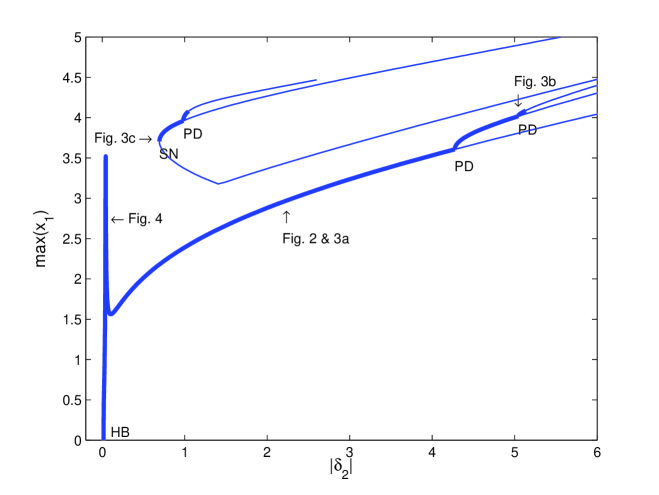
Figure 1: Numerical bifurcation diagram (AUTO) [18] using $\delta_{2}$ as the bifurcation parameter. Note, the coupling is negative so $\delta_{2}<0$; as we increase $|\delta_{2}|$, the coupling is increasingly negative. Thick (thin) lines indicate that the periodic solutions are stable (unstable). There is an initial Hopf bifurcation (HB) from the steady state to periodic solutions. As $|\delta_{2}|$ is increased the initial periodic orbit exhibits a period-doubling (PD) sequence of bifurcations to chaos; we show only the first two PD bifurcations. Simultaneously, subharmonic periodic solutions appear through saddle-node (SN) bifurcations and will also period double. For these parameter values, $|\delta_{2S}|>|\delta_{2H}|$ so that the small-coupling feedback resonance peak is exhibited. (Fixed parameters are $\epsilon=0.001$, $b_{1}=b_{2}=1$, $a_{1}=a_{2}=25$ and $\delta_{1}=0.04$.)

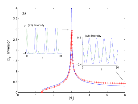
Figure 4: (a) Amplitude of inversion $x_{2}$ as a function of $\delta_{2}=\epsilon d_{2}$ after the Hopf bifurcation; numerical (+) (Auto [18]), analytical from Eq. (17) (solid line). Parameter values are $\epsilon=0.001$, $a_{1}=a_{2}=2$, $d_{1}=3$ and $\alpha=0$ so that $d_{2H}=4/3$ and $d_{2S}=3$. In the inset (a1) we show the pulsating intensity near the peak of the resonance ($y_{1}$ dashed. $y_{2}$ solid), while in inset (a2), the intensity has returned to be small-amplitude and nearly harmonic. (b) Period of oscillations as a function of $\delta_{2}=\epsilon d_{2}$ with analytical result (solid line) from Eq. 19.

In Fig. 1 we show the amplitude of the periodic solutions that emerge from the Hopf bifurcation point of Eq. (9). As the magnitude of the coupling constant $(|\delta_{2}|,\;\;\delta_{2}<0)$ is increased, the Hopf bifurcation leads to small-amplitude periodic solutions. However, for small coupling there is a strong resonance effect where the amplitudes become $O(1)$. In Fig. 1 this appears as a narrow spike in the amplitude. We show a close-up of the amplitude resonance in Fig. 4 (calculated at different parameter values). Both before and after, the amplitude is small and nearly harmonic, as would be expected for weak coupling. However, during the resonance the amplitude is pulsing.

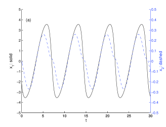
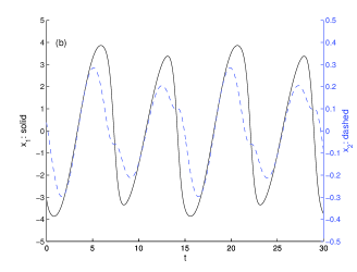
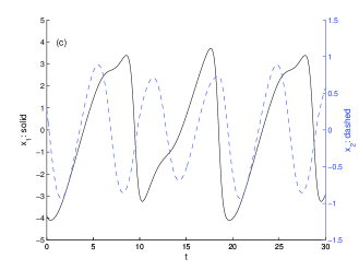
Figure 3: Comparison of the amplitude of the population inversion of laser-1 (left axis, solid curve) and the inversion of laser-2 (right axis, dashed line) for: (a) Before the first period-doubling bifurcation, $|\delta_{2}|=2.18$ (same as Fig. 2). (b) After the period-doubling bifurcation $|\delta_{2}|=5.04$. (c) Just after the saddle-node bifurcation near the limit point, $|\delta_{2}|=0.70$. There are three maximums of laser-2 for every two maximum of laser-1.

As $|\delta_{2}|$ is increased, the coupled system behaves similar to a periodically modulated laser [4, 14]. The intensity of laser-1 increases and becomes pulsating (see Fig. 2a) because the effective modulation signal from laser-2 becomes stronger. On the other hand, because $\delta_{1}$ is fixed and small, laser-2 receives only a weak signal from laser-1 and remains nearly harmonic (see Fig. 2b). For larger coupling, the periodic solutions exhibit a period-doubling sequence to chaos; the inversion for both laser-1 and -2 after the first period-doubling bifurcation is shown in Fig. 3b. We mention also that for different parameter values the original branch of periodic solutions may remain completely stable and not exhibit further bifurcations.

Coexisting with the primary branch of periodic solutions are subharmonic resonances that appear through saddle-node bifurcations. These also exhibit period-doubling bifurcations for increasing coupling. In Fig. 3c we see that just after the primary saddle-node bifurcation the periods of the oscillations are in a 2:3 ratio, with 2 maximum of laser-1 for every 3 of laser-2.

3 Weak-coupling resonance

3.1 Two lasers

We now describe the periodic solutions that emerge from the Hopf bifurcation located by Eq. (9). We use the standard method of multiple time-scales [13] approach and thus only summarize the results. From the linear-stability analysis, we know that solutions decay on an $O(\epsilon)$ time scale. This suggests that we introduce the slow time $T=\epsilon t$, such that $x=x(t,T)$ (similarly for $y$) and time derivatives become $\frac{d}{dt}=\frac{\partial}{\partial t}+\gamma^{2}\frac{\partial}{\partial T}$. We analyze the nonlinear problem using perturbation expansions in powers of $\epsilon^{1/2}$, e.g., $x_{j}(t)=\epsilon^{1/2}x_{j1}(t,T)+\epsilon x_{j2}(t,T)+\ldots$, Finally, we assume that the coupling constants are small and let $\delta_{j}=\epsilon d_{j}$.

At the leading order, $O(\epsilon^{1/2})$, we obtain the solutions

$$y_{j1}(t,T)=A_{j}(T)e^{it}+c.c.,\quad x(t,T)=iA_{j}(T)e^{it}+c.c.,$$ (11)

which exhibit oscillations with radial frequency 1 on the $t$ time scale. To find the slow evolution of $A_{j}(T)$ we must continue the analysis to $O(\epsilon^{3/2})$. Then, to prevent the appearance of unbounded secular terms, we determine “solvability conditions” for the $A_{j}(T)$ that are given by

$$\frac{dA_{1}}{dT} = -\frac{1}{2}a_{1}A_{1}-\frac{1}{6}i|A_{1}|^{2}A_{1}-\frac{1}{2}id_{2}A_{2},$$ (12)

$$\frac{dA_{2}}{dT} = -\frac{1}{2}a_{2}A_{2}-\frac{1}{6}i|A_{2}|^{2}A_{2}-\frac{1}{2}id_{1}A_{1}+i\alpha A_{2}.$$ (13)

To analyze these equation we let $A_{j}(T)=R_{j}(T)e^{i\theta_{j}(T)}$ and consider the phase difference $\psi=\theta_{2}-\theta_{1}$ to obtain

$$\frac{dR_{1}}{dT} = -\frac{1}{2}a_{1}R_{1}+\frac{1}{2}\sin(\psi)d_{2}R_{2},$$ (14)

$$\frac{dR_{2}}{dT} = -\frac{1}{2}a_{2}R_{2}-\frac{1}{2}\sin(\psi)d_{1}R_{1},$$ (15)

$$\frac{d\psi}{dT} = -\frac{1}{6}(R_{2}^{2}-R_{1}^{2})-\frac{1}{2}\cos\psi(d_{1}\frac{R_{1}}{R_{2}}-d_{2}\frac{R_{2}}{R_{1}})+\alpha.$$ (16)

The leading order, solutions are $t=2\pi$ periodic if the amplitudes and phase are constant with respect to the $T$ time scale (derivatives with respect to $T$ are zero). This determines the bifurcation equation for the amplitudes $R_{j}$ and the phase difference $\psi$ as

$$R_{2}^{4}=-9\frac{\Delta_{1}}{\Delta_{2}^{2}},\mbox{ where }\Delta_{1}=(1+\frac{d_{1}d_{2}}{a_{1}a_{2}})(a_{1}+a_{2})^{2},\mbox{ and }\Delta_{2}=1+\frac{a_{2}d_{2}}{a_{1}d_{1}},$$ (17)

and

$$R_{1}^{2}=-\frac{a_{2}d_{2}}{a_{1}d_{1}}R_{2}^{2},\;\cos^{2}\psi=(1+\frac{a_{1}a_{2}}{d_{1}d_{2}}),$$ (18)

where we have set $\alpha=0$ to simplify the discussion. For $R_{1}$ to be positive in Eq. (18), $d_{1}$ and $d_{2}$ must have opposite signs, while the Hopf bifurcation point is determined by taking $R_{2}\rightarrow 0$ in Eq. (17) to obtain $\Delta_{1}=0$; both conditions are consistent with the linear stability results in Eq. (9). We define the value at which the Hopf bifurcation occurs to be $\delta_{2H}=\epsilon d_{2H}$. For $d_{2}>d_{2H}$, Eq. (18) describes a supercritical bifurcation to stable periodic solutions; this is consistent with the numerical bifurcation diagram in Fig. 1. Finally, because $d\psi/dT=0$, the laser oscillations are phase locked with the phase difference described by Eq. (18), and the frequency for $x$ and $y$ is

$$\omega=1-\frac{\epsilon}{2}\sqrt{-\Delta_{1}}\left(\frac{1}{|\Delta_{2}|}+\frac{a_{2}}{a_{1}+a_{2}}\right)+O(\epsilon^{3/2}).$$ (19)

An important result of this paper comes from an examination of $\Delta_{2}$ in Eq. (17). Specifically, the bifurcation equation is singular when $\Delta_{2}=0$ or

$$d_{2}=d_{2S}\equiv-\frac{a_{1}}{a_{2}}d_{1}.$$ (20)

If $d_{2S}<d_{2H}$, then the singularity occurs before the Hopf bifurcation when the CW steady-state is still stable. Thus, in this case, the singularity is not seen and does not affect the amplitude of the bifurcating periodic solutions. However, if $d_{2S}>d_{2H}$, then near the bifurcation point the amplitude of the oscillations becomes very large corresponding to a resonance. The resonance can be understood as a balance between an effective negative damping due to the coupling term, and the self damping. That is, the ratio $d_{2}/a_{1}$, which is the relative negative camping to the self damping in laser-1, is equivalent to $d_{1}/a2$ (modulus the negative sign), the relative negative damping to self damping in laser-2. The net result is that the coupling terms provide an effective negative-damping that cancels with the lasers self-damping and, hence, a resonance effect.

The negative-coupling resonance when $d_{2}=d_{2S}$ is demonstrated in Fig. 4a. The solid line is the result of our analytical bifurcation curve given by Eq. (17), while the $+$ are data from numerical simulation; the analytical and numerical results are in excellent agreement. In the vicinity of $\delta_{2}=\delta_{2S}$ the amplitude of the periodic oscillations become $O(1)$, whereas we would normally expect the amplitude to remain $O(\epsilon^{1/2})$.

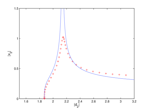
Figure 5: Amplitude of $x_{2}$ as a function of $\delta_{2}=\epsilon d_{2}$ after the Hopf bifurcation; numerical (+) [18], analytical (solid line). The parameters have been chosen as $a_{2}=2.9$ and $d_{1}=3.1$ so that the singular point $d_{2S}=2.13$ is very near the Hopf bifurcation $d_{2H}=1.87$.

Comparing Fig. 4a and Fig. 5, we see that the maximum amplitude, when $\delta_{2}=\delta_{2S}$, depends on the parameters. However, the bifurcation equation is singular at $\delta_{2S}$ and does not give a value for the maximum. The bifurcation equation can be improved by tuning the resonance closer to the Hopf bifurcation point with $\delta_{1}=\epsilon a_{2}+O(\epsilon^{3/2})$ and $\delta_{2}=-\epsilon a_{1}+O(\epsilon^{3/2})$ and continuing the perturbation analysis to $O(\epsilon^{2})$. Unfortunately, the analysis become algebraically difficult and we have not pushed through to its conclusion.

During the resonance both lasers become pulsating. Pulsating solutions are not well described by the weakly-nonlinear analysis of the present section. In Appendix A we consider pulsating lasers and again locate the resonance peak at $\delta_{2S}$. We discuss this further in the paper’s final discussion section.

3.2 Three (or more) lasers

The resonance spike can also be found in three or more lasers. In general, the amplitudes of the periodic solutions near the Hopf bifurcation are described by coupled Stuart-Landau equations of the form

$$\frac{dA_{j}}{dT}=-\frac{1}{2}a_{j}A_{j}-\frac{1}{6}i|A_{j}|^{2}A_{j}-\frac{1}{2}i\sum_{k=1,k\neq j}^{N}d_{jk}A_{k},\quad j=1\ldots N.$$ (21)

As written, the coupling coefficients are completely general and could be chosen to give global coupling, $d_{jk}=d$, nearest-neighbor coupling, $d_{j,k}\neq 0$ for only $k=j+1,\;\;k=j-1$, or any other coupling configuration. Coupled algebraic equations for the amplitudes $R_{j}$ can then be found with the substitution $A_{j}=R_{j}\exp(i\theta_{j})$. An amplitude resonance occurs when there is a vanishing denominator in the equation for any one of the isolated amplitudes $R_{j}=g(R_{k}),\;\;k\neq j$. As with two lasers, one of the coupling constants must be negative to produce the resonance. However, obtaining an explicit solution for one of the laser amplitudes, even in the case of only three lasers, is extremely difficult in all but the most trivial cases.

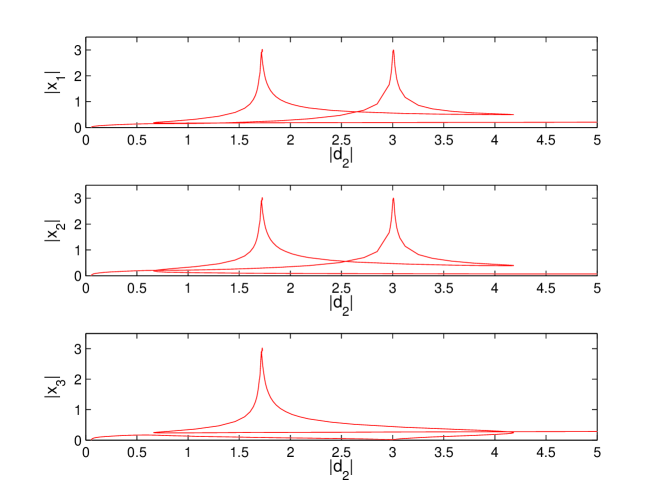
Figure 6: Amplitudes for the case of three identical lasers (fixed parameters are $a_{1}=a_{2}=a_{3}=2$, $b=1$, $\beta_{1}=\beta_{2}=1$, $\epsilon=0.001$.) The fixed-coupling contants are $\delta_{13}=\delta_{23}=1.3$ and $\delta_{21}=\delta_{31}=3$. The coupling of laser-2 into laser-3 is positive with size $\delta_{32}=|\delta_{2}|$, while the coupling of laser-2 into laser 1 is negative with $\delta_{12}=\delta_{2}<0.$

In contrast, demonstrating the resonance effect numerically requires only some experimentation and we show one result in Figs. 6 and 7. In Fig. 6 we show the amplitude of each laser as a function of one of the coupling parameters. Specifically, we fix the coupling of laser-3 into laser-1 and laser-2 as $d_{13}=d_{23}=1.3$ and the coupling of laser-1 into laser-2 and laser-3 as $d_{21}=d_{31}=3$. The coupling of laser-2 into laser-3 is positive with size $d_{32}=|d_{2}|$, while the coupling of laser-2 into laser-1 is negative with $d_{12}=d_{2}<0.$ We use $d_{2}$ as the control parameter.

As $|d_{2}|$ is increased, both laser-1 and laser-2 show two resonance peaks, while for laser-3 there is only one. However, in Fig. 7 we see that the branch of solutions is not monotonic in $|d_{2}|$. As the branch of solutions is followed from the Hopf bifurcation point, the resonance peak for larger $|d_{2}|\approx 3$ occurs first, but only for laser-1 and laser-2. As the branch is followed further, it turns at the saddle-node bifurcation (right most in figure). As $|d_{2}|$ decreases, all three lasers exhibit a resonance when $|d_{2}|\approx 1.75$. The branch turns again at a saddle-node bifurcation (left most) to then increase without any further resonances.

As it happens, the periodic solutions are unstable on the branch of solutions with the lower resonance peak $|d_{2}|\approx 1.75$. Thus, between the two saddle-node bifurcations there are two stable solutions: the primary branch originating from the Hopf bifurcation that exhibits a resonance for laser-1 and laser-2 and terminates at the larger (right) saddle-node bifurcation, and the small-amplitude branch that appears at the lower (left) saddle-node bifurcation and continues for $|d_{2}|>5$. Thus, in the vicinity of the resonance when $|d_{2}|\approx 3$ and both stable solutions coexist, initial conditions will determine whether the large-amplitude resonant solutions or the small-amplitude solutions are exhibited

Finally, the period of the oscillations shows a sharp peak at each of the amplitude resonances. The result is analogous to that of the peak in the period for two lasers as shown in Fig. 4b.

4 Strong coupling

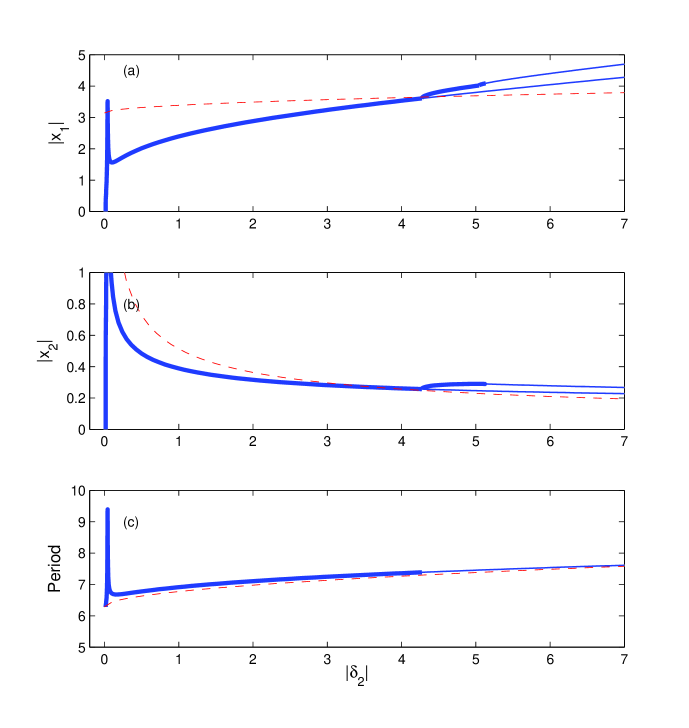
Figure 8: Comparison of numerical bifurcation results (solid) to the analytical results (dashed) from the map in Sec. 4, specifically, Eqs. (41). Parameters are the same as in Fig. 1.

For “large” values of the coupling, when $\delta_{2}=O(1)$, the intensity of laser-1 becomes pulsating, while the oscillations of laser-2 remain small and nearly harmonic (see Fig. 2). We derive an iterated map to describe the oscillations when $\delta_{2}=O(1)$. Fixed points of the resulting map correspond to periodic solutions of Eq. (6). Our results are summarized in Fig. 8, where we compare the amplitudes and period to those obtained from numerical simulation.

To construct the map we take advantage of the fact that the intensity of laser-1 has two distinct regimes: during the pulse when $y_{1}\gg 1$, and a long interval of time when $y_{1}\approx-1$. For a single pulsating laser, the solutions to Eq. (6) have described using an iterated map constructed with the method of matched asymptotics [4, 14]; we will use the same approach here and so will just summarize our results. We will first find the “outer” solutions to Eqs. (6) with the approximation $y_{1}\approx-1$ ( see Fig. 2a from $t_{0}$ to $t_{1}$). We will then reanalyze the coupled system with an “inner” or “boundary-layer” approximation $y_{1}\gg 1$ (see Fig. 2a from $t_{1}$ to $t_{2}$). The typical next step is to match the inner and outer solutions to form a composite solution over the whole period. However, we are interested in the dynamics from one pulse to the next. Hence, we will simply patch the solutions together to form an iterated map.

As described above, the pulsations of laser-1 define the inner and outer regimes. However, laser-2 continues to exhibit small-amplitude, nearly-harmonic oscillations. Thus, in each regime we will use the method of multiple scales to describe the oscillations of laser-2.

4.1 Re-supply of the inversion, $y_{1}\approx-1$

We first consider the outer regime when $y_{1}\approx-1$. We define $t=t_{0}$ as the time of completion of a previous pulse, when $y_{1}=0$ and the inversion $x_{1}$ is at its minimum (see Fig. 2). The end of the outer regime will be defined to be when the intensity increases from $y_{1}=-1$ back to $y_{1}=0$ and the inversion $x_{1}$ is at its maximum.

We first consider laser-2. When $y_{1}\approx-1$ the dynamics of laser-2 can be approximated as

$$\frac{dy_{2}}{dt} = \beta x_{2}(1+y_{2}),$$

$$\frac{dx_{2}}{dt} = \beta[-y_{2}-\epsilon\beta x_{2}(a_{2}+by_{2})-\delta_{1}],$$ (22)

We can solve this system using the method of multiple scales as we did in Sec. 3.1 under the assumption that $\delta_{1}$ is small ($\delta_{1}=O(\epsilon)$). We find that to leading order laser-2 is a weakly damped, nearly harmonic oscillator described as

$$x_{2}(t) = e^{-\frac{1}{2}\epsilon a_{2}\phi},[x_{20}\cos(\omega\phi)-y_{20}\sin(\omega\phi)],\;\;\;\phi=t-t_{0},$$

$$y_{2}(t) = -\frac{dx_{2}}{dt},$$

$$\omega = 1-\frac{1}{2}\delta_{1}-\frac{1}{24}(x_{20}^{2}+y_{20}^{2})e^{-\epsilon a_{2}\phi},$$ (23)

where $(x_{2}(t_{0}),y_{2}(t_{0}))=(x_{20},y_{20})$ is the state of laser-2 at the end of the previous pulse. (As in Sec. 3.1, $x_{2}$ and $y_{2}$ are $O(\epsilon^{1/2})$ such that the next term in the solutions in Eqs. (23) would be $O(\epsilon)$.)

We now examine laser-1 in more detail. With $y_{1}\approx-1$ we have

$$\frac{dx_{1}}{dt}=1-\epsilon(a_{1}-b)x_{1}+\delta_{2}y_{2},$$ (24)

which can be integrated to obtain

$$x_{1}(t)=(x_{10}-\frac{1}{\gamma})e^{-\gamma\phi}+\frac{1}{\gamma}+\delta_{2}e^{-\gamma t}\int_{t_{0}}^{t}e^{\gamma s}y_{2}(s)ds,$$ (25)

where $\gamma=\epsilon(a_{1}-b)$. Using the result for $y_{2}$ from Eqs. 23 we obtain

$$x_{1}(t) = (x_{10}-\frac{1}{\gamma})e^{-\gamma\phi}+\frac{1}{\gamma}$$ (26)

$$+\frac{\delta_{2}}{\alpha^{2}+\omega^{2}}e^{-\gamma\phi}\left[(\alpha y_{20}-\omega x_{20})(e^{\alpha\phi}\cos(\omega\phi)-1)\right.$$

$$\quad\quad\quad\quad\quad\quad\quad\left.+(\omega y_{20}+\alpha x_{20})e^{\alpha\phi}\sin(\omega\phi)\right],$$

where $\alpha=(\gamma-\epsilon a_{2}/2)$. We can now use $x_{1}$ to improve our approximation for $y_{1}$ by substituting Eq. (26) in the equation for $y_{1}$ in Eq. (6); we then integrate to give

$$y_{1}(t)=-1+(1+y_{10})\exp\left(\int_{t_{0}}^{t}x_{1}(s)ds\right).$$ (27)

During the outer regime the inversion grows almost linearly from its minimum to maximum values, more precisely, for $\epsilon\ll 1$, $x_{1}\approx(t-t_{0})$. With the inversion re-supplied the laser can then emit a new pulse of light. We define the start of the next pulse at $t=t_{1}$ to be when $y_{1}(t_{1})=0$. Thus, the next pulse begins when the integral in the exponential of Eq. (27) is zero, or

$$\int_{t_{0}}^{t_{1}}x_{1}(t)dt=0.$$ (28)

4.2 Pulse regime, $y_{1}\gg 1$

The inner regime is defined to be when the intensity is large, $y_{1}\gg 1$, and occurs over a very short interval of time. Specifically, if $y_{1}=O(E)$, where $E\gg 1$ is related to the energy, then $x_{1}=O(E^{1/2})$ and the width of the pulse is $O(1/E^{1/2})$ [14]. On the other hand, the oscillations of laser-2 remain small, $O(\epsilon^{1/2})$. Thus, we assume that to leading order, laser-2 has no effect on laser-1 during the pulse. We can then use the results from [14], in the absence of modulation, to describe laser-1. Namely, (i) the end of the pulse, $t=t_{2}$, is defined to be when the pulse intensity returns to zero, $y(t_{2})=0$, (ii) the width of the pulse is negligible compared to the time in the outer regime, $(t_{2}-t_{1})\approx 0$, and (iii) the inversion drops from its maximum to minimum value with reduction due to damping:

$$x_{1}(t_{2})=-x_{1}(t_{1})+\frac{2}{3}\epsilon bx_{1}(t_{1})^{2}.$$ (29)

($x_{1}(t_{2})$ is negative at the minimum so that the additional positive term is a reduction in the magnitude of the minimum.)

The large and narrow ($t=O(1/E^{1/2})$) pulse of laser-1 does have a significant effect on laser-2. To determine the appropriate inner problem for laser-2, we scale the pulse amplitude as $y_{1}=O(E)$ and stretch time according to $t=O(1/E^{1/2})$. The coupling is weak with $\delta_{1}=O(\epsilon)$. Finally, we assume that $E=O(1/\epsilon^{1/2})$ to obtain

$$\frac{dx_{2}}{dt} = \delta_{1}y_{1},$$

$$\frac{dy_{2}}{dt} = 0.$$ (30)

Thus, to leading order $y_{2}$ is constant during the pulse while $x_{2}$ is given by

$$x_{2}(t_{2})-x_{2}(t_{1})=\delta_{1}\int_{t_{1}}^{t_{2}}y_{1}(t)dt.$$ (31)

However, in the pulsing regime we have that $dx_{1}/dt\approx-y_{1}$ so that

$$x_{2}(t_{2})-x_{2}(t_{1})=-\delta_{1}\int_{t_{1}}^{t_{2}}\frac{dx_{1}}{dt}dt=\delta_{1}[x_{1}(t_{1})-x_{1}(t_{2})].$$ (32)

Thus, for laser-2 we have that

$$x_{2}(t_{2})=x_{2}(t_{1})+\delta_{1}2x(t_{1}),\quad y(t_{2})=y(t_{1})$$ (33)

where we have used Eq. (29) in Eq. (32) and kept only the leading order terms (the leading order is $O(\epsilon^{1/2})$ and we have dropped the $O(\epsilon)$ corrections). The net effect is that at the end of the pulse when $t=t_{2}$, the intensity $y_{2}$ remains unchanged, while $x_{2}$ has received a “kick” due to the pulse from laser-1.

4.3 Constructing the map

To construct a map, we “patch” together the results from the outer and inner analysis of the previous two sections.

For laser-2 we initially have $(x_{2}(t_{0}),y_{2}(t_{0}))=(x_{20},y_{20})$ that in the outer region evolves according to Eqs. (23) until $t=t_{1}$. Then, in the inner region, laser-2 receives the pulse from laser-1 according to Eq. 33. Thus, we have that

$$\left[(x_{2}(t_{0}),y_{2}(t_{0}))=(x_{20},y_{20})\right]\mapsto(x_{2}(t_{1}),y_{2}(t_{1}))\mapsto(x_{2}(t_{2}),y_{2}(t_{2})).$$ (34)

The total time from one pulse to the next is $t_{2}-t_{0}$. However, because the pulse is so short ($O(\epsilon^{1/2})$), we make the approximation that $t_{2}\approx t_{1}$ and define the total time as $P=t_{1}-t_{0}$. Finally, for notation convenience we define the intermediate value of the inversion of laser-1 as $G(P)=x_{1}(t_{1})$. The map for laser-2 is then

$$x_{2} \mapsto e^{-\frac{1}{2}\epsilon a_{2}P}[x_{2}\cos(\omega P)-y_{2}\sin(\omega P)]+\delta_{1}2G(P),$$

$$y_{2} \mapsto e^{-\frac{1}{2}\epsilon a_{2}P}[x_{2}\sin(\omega P)+y_{2}\cos(\omega P)],$$ (35)

where

$$G(P) = (x_{1}-\frac{1}{\gamma})e^{-\gamma P}+\frac{1}{\gamma}$$ (36)

$$+\frac{\delta_{2}}{\alpha^{2}+\omega^{2}}e^{-\gamma P}\left[(\alpha y_{2}-\omega x_{2})(e^{\alpha P}\cos(\omega P)-1)+(\omega y_{2}+\alpha x_{2})e^{\alpha P}\sin(\omega P)\right].$$

The time from one pulse to the next is determined when $y_{1}=0$ with $t_{2}\approx t_{1}$. Thus, from Eq. (28) we have a condition to determine $P$ as

$$\int_{0}^{P}G(t)dt=0.$$ (37)

Finally, for the inversion of laser-1 we have

$$x_{1}(t_{0})\mapsto[x_{1}(t_{1})=G(P)]\mapsto x_{1}(t_{2}),$$ (38)

yielding

$$x_{1}\mapsto-G(P)+\frac{2}{3}\epsilon bG(P)^{2}.$$ (39)

The map is evaluated as follows: (i) The current state of the system, given by $x_{1}$, $x_{2}$ and $y_{2}$, is known. (ii) Compute the time $P$ of the next pulse using Eq. (37). (iii) With $P$ fixed we can evaluate $G(P)$ in Eq. (36). (iv) The current state of the system and $G(P)$ determine new values for $x_{2}$ and $y_{2}$ with Eqs. (35). (v) Finally, $x_{1}$ is found from Eq. (39). Summarizing, we have

(ii) Eq. (37) $$f_{1}(P;x_{1},x_{2},y_{2})=0,$$

(iv) Eq. (35) $$x_{2}\mapsto f_{2}(x_{2},y_{2},G(P))$$

$$y_{2}\mapsto f_{3}(x_{2},y_{2},G(P))$$

(v) Eq. (39) $$x_{1}\mapsto f_{4}(G(P)).$$ (40)

4.4 Periodic solutions as fixed points

Fixed points of the map described by Eqs. (40) correspond to periodic solutions of the original flow, Eqs. (6). However, it is not feasible to analyze the map without further approximations. We will look for fixed points making use of $\epsilon\ll 1$. With heavy use of symbolic computation, we find that the maximum amplitudes and the period of the oscillations are given by

$$\max[x_{1}] = \pi+\sqrt{\frac{3a_{2}}{2a_{1}}\delta_{1}|\delta_{2}|},$$

$$\max[x_{2}] = \max[y_{2}]=\sqrt{\pi^{2}\frac{2a_{1}}{3a_{2}}\frac{\delta_{1}}{|\delta_{2}|}},$$

$$P = 2\max[x_{1}].$$ (41)

For each result the neglected terms are $O(\epsilon)$. In addition, we also obtain the phase relationship result that $x_{2}\approx 0$ when $x_{1}$ is at its minimum, which is consistent with Fig. 2. We have plotted the predictions of Eqs. (41) along with the results from numerical simulations in Fig. 8 and they show good agreement, where for clarity we have removed the higher bifurcation branches present in Fig. 1.

The period $P$ and the amplitude of laser-2 show excellent agreement. We see that $\max[x_{2}]\approx 1/|\delta_{2}|^{1/2}$. This may initially seem counter intuitive because the pulses of laser-1 grow with $|\delta_{2}|$ and provide a greater kick to laser-2. Indeed, a leading-order approximation to the kick applied by laser-1 $\delta_{1}2G(P)\approx\delta_{1}P$, thus, the strength of the kick increases as the period increases. However, with longer periods the exponential decay due to damping in the outer regime has more time to decrease the amplitude of laser-2. The net effect is a decrease in $\max[x_{2}]$ with increasing $|\delta_{1}|$.

The net coupling strength of laser-2 to laser-1, with respect to $|\delta_{2}|$, is $\delta_{2}y_{2}=O(\delta_{2}^{1/2})$. Thus, the amplitude of the pulsations increases with increasing $\delta_{2}$. The fit between the analysis and numerics is not as good for laser-1. To achieve a better fit we need to derive a map that includes higher-order terms in $\epsilon$, which we have not attempted.

5 Discussion

For two coupled lasers we have studied the bifurcations that occur when the coupling constants are of opposite sign and unequal. Specifically, the coupling is asymmetric in that we fix one coupling constant ($\delta_{1}>0$) to be small, while varying the other ($\delta_{2}<0$). There are two Hopf bifurcations to periodic output, one for $\delta_{2}$ positive and one for $\delta_{2}$ negative. We have focused our attention on the latter because of its similarity to our work with delay coupling in [1]. When the output of laser-2 is nearly harmonic, the negative coupling effectively corresponds to phase shift by half of a period. This is equivalent to delayed coupling when the delay is half the period.

As $|\delta_{2}|$ is increased there is an initial Hopf bifurcation from the laser’s CW steady-state to periodic solutions. We then observe two resonance regimes where the coupled system shows novel and interesting output. (i) Close to the Hopf bifurcation a resonance can occur where the amplitude of the laser oscillations becomes large. This is unexpected because both coupling constants are still small. The resonance is due to the negative-coupling that effectively reduces the damping in the laser. (ii) As the strength of the coupling increases further the periodic solutions may, depending on the parameters, exhibit a period-doubling sequence to chaos as well as the coexistence of subharmonic solutions. These effects are reminiscent of a periodically modulated laser. In the case of the coupled lasers the laser receiving the weak coupling remains a nearly harmonic oscillator that excites the strong resonances of the pulsating laser.

The large-amplitude resonance that occurs for small coupling can be easily understood from the well-known coupled Stuart-Landau equations given generically by Eq. (21). Steady-state solutions of Eq. (21) correspond to the amplitude of the periodic solutions. Simple algebra shows that tuning some of the coupling parameters to be of opposite sign can lead to a vanishing denominator. Physically, the coupling term is providing an effective negative-damping that cancels with the lasers self-damping and, hence, a resonance effect. Our analysis assumed that both coupling constants were of the same relative size, $\delta_{j}=O(\epsilon)$. However, other scalings satisfy the Hopf condition, e.g., $\delta_{1}=O(\epsilon^{1/2})$ and $\delta_{2}=O(\epsilon^{3/2}$. This does not change the qualitative properties of the bifurcating periodic solutions in any way.

In App. A we have attempted to describe the solutions that occur near the peak of the resonance. In this regime, both lasers show approximately equal amplitude pulsating solutions as exhibited by Fig. 4(a1). Our analysis reproduces the equation for the location of the resonance $\delta_{2S}$. It also predicts that the period should be twice the maximum amplitude of the inversion. That both the period and the amplitude show a resonance peak at $\delta_{2S}$ in Fig. 4a & b is consistent with this result but the scale factor of 2 is not correct. Also, we do not obtain and expression for how the period (or amplitude) depends on the parameter $\delta_{2}$. A difficult higher order analysis would be required to remedy these last two limitations.

In Fig. 2 we showed that when $|\delta_{2}|=O(1)$ (see Fig. 1) that one of the lasers amplitudes is large while the other’s remains small. The term “localized solutions” has been used to describe the case when identical oscillators in a coupled system exhibit amplitudes of different scales. In coupled lasers localized solutions have been described by Kuske and Erneux [15] who derived a similar pair of integral conditions to Eq. (42). Instead of looking for pulsating solutions, they considered $O(1)$ solutions approximated using a Poincare-Lindstedt method, and small amplitude solutions approximated with the method of multiple scales. Repeating this analysis for our problem reproduces the Hopf bifurcation results that we obtained in Sec. 3.

To describe the system’s output when the coupling is strong, we have derived a map that predicts the period, amplitude and phase of the lasers from one pulse of laser-1 to the next. Constructing the map relies on combining both strongly and weakly nonlinear asymptotic methods. That is, we used matched asymptotics to describe the pulsating laser-1 and to separate one period into an inner and outer subintervals. For the small-amplitude laser-2 we used the multiple scale methods within each subinterval. We obtain very good agreement between the amplitude of laser-2 and the overall period. The amplitude of the pulsations of laser-1 are not described quite as well. This could be because we need to consider higher-order terms in our solutions, or we are comparing our numerical and analytical results in a less than ideal parameter regime.

The large-amplitude solutions in the resonance peak just after the Hopf bifurcation are not the same as those that appear due to a “singular-Hopf bifurcation” [17, 16]. In the latter case, the large amplitude oscillations are due to crossing a separatrix separating small-amplitude solutions near the Hopf bifurcation from large-amplitude relaxation oscillations formed around a slow manifold. The functional form of the dissipation terms in the present problem disallows this type of behavior.

To our knowledge, the small-coupling resonance peak has not been previously described; most likely this due to consideration of physical systems where controlling the sign of the coupling is not possible. However, in a forthcoming study we will show that for same-sign coupling but with delay, we can again produce the resonance because the delay provides the phase shift that effectively leads to the sign change.

Appendix A Pulsating solutions for weak coupling

In Sec. 3 we looked for small-amplitude solutions near the Hopf bifurcation point. We now allow the amplitude of the solution to be arbitrary but will still consider the coupling to be small. The laser system Eq. (6) can be rewritten so that the intensity and inversion evolve according to a perturbed-Hamiltonian system [14]. From the coupled-Hamiltonian systems, we derive solvability conditions for T-periodic solutions as

$$\int_{0}^{T}(-a_{j}x_{j}^{2}+d_{k}x_{j}y_{k})dt=0,$$ (42)

The integrals in Eq. (42) are computed by evaluating $x_{j}$ and $y_{j}$ on periodic orbits of the $\epsilon=0$, Hamiltonian system. Unfortunately, we do not have closed form analytical solutions for $x_{j}$ and $y_{j}$. However, for pulsating output we can construct approximate solutions to the Hamiltonian system using matched asymptotic expansions similar to what we did in Sec. (4). In this case, we match the outer and inter solutions to determine a uniform solution that can be used to evaluate the integrals in Eq. (42). Because we have carried out similar calculations in the past [4, 14], we will only summarize the details of the intermediate steps.

Before proceeding, we mention that Kuske and Erneux [15] derived an almost equivalent pair of solvability conditions for two coupled lasers. Their goal was to investigate so-called “localized” solutions where one laser has $O(1)$ amplitude oscillations, while the other has small oscillations, and both are approximated using the Poincare’-Linstedt perturbation method. Doing this calculation for our problem effectively reproduces our earlier results obtained near the Hopf bifurcation point and thus does not provide new information.

We assume that laser-$j$ has period $T_{j}$, which is some fraction of the total period with $T=n_{j}T_{j}$. The first term in each integral is $x_{j}^{2}$ and because it does not involve the other laser is independent of the phase relationship between lasers $j$ and $k$. Thus, using the results from [14] we have

$$\int_{0}^{T}x_{j}^{2}dt=\frac{n_{j}}{12}T_{j}^{3}.$$ (43)

Integrating $x_{j}y_{k}$ is more complicated because we must allow for a phase difference, $T_{\phi}$, between the two pulsating lasers. However, it is easy to predict the form of the result. The intensity $y_{k}$ is pulsating and acts like a delta function that samples the inversion $x_{j}$ at the time of the pulse. The effect of the integral is to sum all of the sample values of the population inversion. In effect, we have a pulse train due to one laser sampling the population inversion of the other. After carrying out the detailed calculations based on the approximate solutions of the Hamiltonian system, we obtain our final result for both solvability conditions:

$$-a_{1}\frac{n_{1}}{12}T_{1}^{3}+T_{2}\delta_{2}\sum_{k=0}^{n_{2}-1}x_{1}((k+\frac{1}{2})T_{2})=0,$$ (44)

where

$$x_{1}(t)=\left\{\begin{array}[]{cc}-jT_{1}+T_{\phi}+t,&jT_{1}-T_{\phi}<t\leq(j+\frac{1}{2})T_{1}-T_{\phi}\\ -(j+1)T_{1}+T_{\phi}+t,&(j+\frac{1}{2})T_{1}-T_{\phi}<t\leq(j+1)T_{1}-T_{\phi}\end{array}\right.,$$ (45)

and

$$-a_{2}\frac{n_{2}}{12}T_{2}^{3}+T_{1}\delta_{1}\sum_{j=0}^{n_{1}-1}x_{2}((j+\frac{1}{2})T_{1}-T_{\phi})=0,$$ (46)

where

$$x_{2}(t)=\left\{\begin{array}[]{cc}-kT_{2}+t,&kT_{2}<t\leq(k+\frac{1}{2})T_{2}\\ -(k+1)T_{2}+t,&(k+\frac{1}{2})T_{2}<t\leq(k+1)T_{2}\end{array}\right..$$ (47)

The inversion variable $x_{j}$ of each laser is a saw-toothed type function that increases linearly from the time of the previous pulse to the next. Specifically, for laser-2, $x_{2}$ increases from 0 (at time $kT_{2}$) to $x_{2}=T_{2}/2$. The intensity pulse depletes the inversion to $x_{2}=-T_{2}/2$, whereupon $x_{2}$ then increases linearly back to 0. Laser-1 is the same except that we must allow for a phase time $T_{\phi}$ between the two lasers.

We consider the simple case of a 1:1 resonance between the lasers where $T=T_{1}=T_{2}$ so that $n_{1}=n_{2}=1$. The solvability conditions reduce to

$$-\frac{a_{1}}{12}T^{2}+\delta_{2}x_{1}(\frac{T}{2})=0$$ (48)

$$-\frac{a_{2}}{12}T^{2}+\delta_{1}x_{2}(\frac{T}{2}-T_{\phi})=0$$ (49)

Because we are interested in periodic solutions, it is sufficient to consider $0\leq T_{\phi}\leq T$. Then, substituting for $x_{1}$ and $x_{2}$, the conditions reduce to

$$-\frac{a_{1}}{12}T^{2}+\delta_{2}(-\frac{T}{2}+T_{\phi})=0$$ (50)

$$-\frac{a_{2}}{12}T^{2}+\delta_{1}(\frac{T}{2}-T_{\phi})=0$$ (51)

After eliminating the phase $T_{\phi}$, we obtain

$$(1+\frac{a_{2}\delta_{2}}{a_{1}\delta_{1}})T^{2}=0.$$ (52)

For periodic solutions with $T\neq 0$, we are forced to set the term in parenthesis equal to zero. This is exactly the same condition that identifies the location of the singularity in the Hopf bifurcation equation (20). This confirms that there is an equal-amplitude, pulsating 1:1 resonance between the lasers when $\delta_{2}=\delta_{2S}$. However, we do not have any information on the period or amplitude, which would require continuing the analysis to higher order.

Figure 2: For $|\delta_{2}|=2.18$ ($\delta_{2}<0$). (a) Laser-1 has pulsating intensity (solid) and a triangular-shaped population inversion (dashed) because it is strongly modulated by laser-2. (b) Laser-2 is nearly harmonic because it receives only weak coupling from laser-1. In (a), the times marked $t_{0}$, $t_{1}$ and $t_{2}$ define the outer and inner regimes discussed in Sec. 4.

Figure 7: Same data as Fig. 6 but with the amplitudes of laser-1 and laser-3 shown simultaneously. The solid curve shows the stable solutions that appear after the Hopf bifurcation (HB). There is a stable resonance peak for $|d_{2}|\approx 3$. The dashed curve shows unstable solutions that exist between the two saddle-node (SN) bifurcations. There is an unstable resonance peak for $|d_{2}|\approx 1.75$. Both laser-3 and laser-1 (and laser 2) exhibit large amplitudes during the unstable resonance, while only laser-1 (and laser-2) has large amplitude during the stable resonance. The dotted curve is a projection of the actual data into only the laser-1 plane to compare to laser-1 data in Fig. 6. There is bi-stability between the saddle-node (SN) points.

References

- [1] M-Y Kim, R. Roy, J.L. Aron, T.W. Carr and I.B. Schwartz, ”Scaling behavior of laser population dynamics with time-delayed coupling: Theory and experiment,” Phys. Rev. Lett., 94 (2005) 088101.
- [2] F.T. Arecchi, G.L. Lippi, G.P. Poccioni and J.R. Tredicce, ”Deterministic Chaos in Laser with Injected Signal,” Optics Commun., 51 (1984) 308–314.
- [3] N.B. Abraham, P. Mandel and L. M. Narducci, ”Dynamical Instabilities and Pulsations in Lasers,” Prog. Opt.,25 (1988) 3–190.
- [4] I.B. Schwartz and T. Erneux, ”Subharmonic Hysteresis and Period-Doubling Bifurcations for a Periodically Driven Laser,” SIAM J. Applied Math., 54 (1994) 1083–1100.
- [5] T. Erneux and P. Mandel, ”Minimal Equations for Antiphase Dynamics in Multimode Lasers,” Phys. Rev. A, 52 (1995) 4137–4144.
- [6] D.G. Aronson and G.B. Ermantrout and N. Kopell, ”Amplitude Response of Coupled Oscillators,” Physica D, 41 (1990) 403–449.
- [7] S.H. Strogatz, ”From Kuramoto to Crawford: exploring the onset of synchronization in populations of coupled oscillators,” Physica D, 143 (2000) 1–20.
- [8] T. Erneux, S.M. Baer and P. Mandel, ”Subharmonic Bifurcation and Bistability of Periodic Solutions in a Periodically Modulated Laser,” Phys. Rev. A, 35 (1987) 1165–1171.
- [9] I.B. Schwartz and H.L. Smith, ”Infinite Subharmonic Bifurcation in an SEIR Epidemic model,” J. Math Bio., 18 (1983) 233–253.
- [10] R.D. Li, P. Mandel and T. Erneux, ”Periodic and quasiperiodic regimes in self-coupled lasers,” Phys. Rev. A, 41 (1990) 5117–5126.
- [11] L. Fabiny, P. Colet, R. Roy and D. Lenstra, ”Coherence and Phase Dynamics of Spatially Coupled Solid-State Lasers,” Phys. Rev. A, 47 (1993) 4287–4296.
- [12] K. Wiesenfeld, C. Bracikowski, G. James and R. Roy, ”Observation of Antiphase States in a Multimode Laser,” Phys. Rev. Lett., 65 (1990) 1749–1752.
- [13] J. Kevorkian and J.D. Cole, ”Multiple Scale and Singular Perturbation Methods,” (Springer-Verlag, New York 1996).
- [14] T.W. Carr, L. Billings, I.B. Schwartz and I. Triandaf, ”Bi-instability and the global role of unstableresonant orbits in a driven laser,” Physica D, 147 (2000) 59–82.
- [15] R. Kuske and T. Erneux, ”Localized Synchronization of Two Coupled Solid-State Lasers,” Optics Commun., 139 (1997) 125–131.
- [16] S.M. Baer and T. Erneux, ”Singular Hopf Bifurcation to Relaxation Oscillations II,” SIAM J. Appl. Math., 52 (1992) 1651–1664.
- [17] S.M. Baer and T. Erneux, ”Singular Hopf Bifurcation to Relaxation Oscillations,” SIAM J. Appl. Math., 46 (1986) 721–739.
- [18] E.J. Doedel, R.C. Paffenroth, A.R. Champneys, T.F. Fairgrieve, Yu.A. Kuznetsov, B. Sandstede and X. Wang, ”AUTO 2000: Continuation and bifurcation software for ordinary differential equations (with HomCont),” California Institute of Technology, Technical Report (2001).
- [19] A.G. Vladimirov, E.A. Viktorov and P. Mandel, ”Multidimensional quasiperiodic antiphase dynamics,” Phys. Rev. E, 60 (1999) 1616–1629.
- [20] H.G. Winful, ”Instability Threshold for an Array of Coupled Semiconductor Lasers,” Phys. Rev. A”, 46 (1992) 6093-6094.
- [21] A. Hohl, A. Gavrielides, T. Erneux and V. Kovanis, ”Localized Synchronization in Two Coupled Nonidentical Semiconductor Lasers,” Phys. Rev. Lett., 78 (1997) 4745–4748.
- [22] K.S. Thornburg, M. Moller, R. Roy, T.W. Carr, R.D. Li and T. Erneux, ”Chaos and Coherence in Coupled Lasers,” Phys. Rev. E, 55 (1997) 3865–3869.