Mixing and reaction efficiency in closed domains

Abstract

We present a numerical study of mixing and reaction efficiency in closed domains. In particular we focus our attention on laminar flows. In the case of inert transport the mixing properties of the flows strongly depend on the details of the Lagrangian transport. We also study the reaction efficiency. Starting with a little spot of product we compute the time needed to complete the reaction in the container. We found that the reaction efficiency is not strictly related to the mixing properties of the flow. In particular, reaction acts as a “dynamical regulator”.

Keyword: Laminar Reacting Flows; non Asymptotic Propagation
PACS numbers: 05.45.-a; 47.70.Fw

I Introduction

Transport of reacting species advected by laminar or turbulent flows (advection reaction diffusion – ARD – systems), is an issue of obvious interest in many fields, e.g. population dynamics (propagation of plankton in oceanic currents [1]), reacting chemicals in the atmosphere (e.g., ozone dynamics [2]), complex chemical reactions and combustion [3]. For recent interesting experimental studies see Ref. [4].

The simplest non trivial case of ARD is described by a scalar field $\theta({\mathbf{x}},t)$, which represents the concentration of reaction products, such that $\theta$ is equal $1$ in the regions where the reaction is over (the stable phase), and $\theta$ is zero where fresh material is present (the unstable phase). The field $\theta({\mathbf{x}},t)$ evolves according to the following equation:

$$\partial_{t}\theta+({\mathbf{u}}\cdot\nabla)\theta=D_{\mbox{0}}\Delta\theta+{1\over\tau}f(\theta),$$ (1)

where ${\mathbf{u}}$ is a given incompressible velocity field and $D_{\mbox{0}}$ is the molecular diffusion coefficient. Of course the reaction is described by the term $f(\theta)/\tau$ where $\tau$ is the time scale of the chemistry.

The form of the reacting term $f(\theta)$ depends on the problem under investigation; a rather popular case is the so-called Fisher-Kolmogorov- Petrovsky-Piskunov (FKPP) nonlinearity [5] $f(\theta)=\theta(1-\theta)$, which describes the auto-catalytic process $A+B\rightarrow 2A$ (in such a case $\theta$ is the concentration of the species $A$). This nonlinearity belongs to the more general class of FKPP-type non-linearity characterized by having the maximum slope of $f(\theta)$ in $\theta\!=\!0$. Those non-linearity terms give rise to the so called pulled fronts for which front dynamics can be understood by linear analysis, since it is essentially determined by the $\theta(x,t)\approx 0$ region (the front is pulled by its leading edge). In the case of front propagation in reaction-diffusion systems (i.e., with ${\mathbf{u}}=0$) it is possible to show [6] that, for FKPP-like non linearity, a moving front (i.e., an “invasion” of the stable phase, $\theta=1$, in the unstable one, $\theta=0$) develops with propagation speed given by $v_{\mbox{0}}=2\sqrt{D_{\mbox{0}}f^{\prime}(0)/\tau}$.

Another important class of non-linearity terms is the non-FKPP-type, for which the maximal growth rate is not realized at $\theta\!=\!0$ but at some finite value of $\theta$, where the details of the nonlinearity of $f(\theta)$ are important. In this case front dynamics is often referred to as pushed, meaning that the front is pushed by its (nonlinear) interior. At variance with the previous case, the determination of the front speed now requires a detailed non linear analysis. It is not possible to give a general result for the front speed, but only the bound (when ${\mathbf{u}}=0$) $2\sqrt{D_{\mbox{0}}f^{\prime}(0)}\leq v_{\mbox{0}}<2\sqrt{D_{\mbox{0}}\sup_{\theta}\left\{{f(\theta)\over\theta}\right\}}\,$ [6] can be obtained. An important example of non-FKPP-type non-linearity is given by the so called Arrhenius term: $f(\theta)=(1-\theta)e^{-\theta_{c}/\theta}$.

In the following we principally adopt the FKPP-type nonlinearity. However, in order to investigate the relevance of $f(\theta)$, we also discuss the non FKPP-type nonlinearity.

If we suppress the reacting term $f(\theta)/\tau$ in (1) we obtain the advection-diffusion equation which rules the evolution of the concentration $P({\mathbf{x}},t)$ of inert particles

$$\partial_{t}P+({\mathbf{u}}\cdot\nabla)P=D_{\mbox{0}}\Delta P\,.$$ (2)

Let us underline that for both the processes (1) and (2) (reactive and inert transport, respectively), one can face different classes of problems, namely the asymptotic and non asymptotic ones [7].

By asymptotic properties we mean the features of Eqs. (1) and (2) at long times and large spatial scales, i.e., much larger than the typical length $\ell$ of ${\mathbf{u}}$. In such a limit, under rather general conditions [8], Eq. (2) reduces to an effective diffusion equation

$$\partial_{t}P=\sum_{i,j}D_{ij}^{e}\partial^{2}_{ij}P$$ (3)

where the effective diffusion tensor $D_{ij}^{e}$ depends, often in a nontrivial way, on ${\mathbf{u}}$. In a similar way for the ARD problem if we start with a localized region in which $\theta=1$ (elsewhere $\theta=0$), one asymptotically has a front propagation with a front speed $v_{\mbox{f}}$ depending on $\tau$, $D_{\mbox{0}}$ and ${\mathbf{u}}$ [9].

Although the asymptotic problems are well defined from a mathematical viewpoint, sometimes their relevance in real life is rather poor. Often, e.g., in geophysics, the spatial size, $L$, of the system is comparable with the typical length of the flow, $\ell$, so it is not possible to use Eq. (3) for the dispersion of passive inert scalar fields and it is necessary to treat the problem using some indicators able to go beyond the diffusion coefficient. Such a problem had been studied, for example, in Refs. [7, 10] using the Finite Size Lyapunov Exponents which properly characterize the transport mechanism at a given (spatial) scale.
In a similar way, considering cases with $L$ not too large compared with $\ell$, one has nontrivial features also in ARD systems. As an example we can mention Ref. [11] where it had been found that the burning efficiency in a closed domain does not increase for large values of the strength of the velocity field.

As a general remark, we stress that both in inertial and reactive transport the Eulerian turbulence has a minor role. As examples we can mention the Lagrangian chaos, i.e., the irregular behavior of passive tracers also for laminar flow [12] and the poor role of the presence of small scales in the velocity field for front propagation [13].

In this paper we discuss the mixing and reaction efficiency [in Eqs. (2) and (1), respectively] in systems advected by a given velocity field, ${\mathbf{u}}$, in closed domains. For mixing efficiency we intend the capacity of a flow to spread particulate inert material starting from a small region over the whole system domain. When the material is chemically active, the interesting question concerns the times needed to complete the reaction in the system domain, that we call reaction efficiency. At an intuitive level one could expect a link between mixing and reaction efficiency, because both are related to the transport properties of the velocity field, but we show there exist cases in which this relation is very weak.

We will see that for the inert transport problem (2), the mixing efficiency strongly depends on the features of the dynamical system

$${{\mathrm{d}}{\mathbf{x}}\over{\mathrm{d}}t}={\mathbf{u}}\,\,,$$ (4)

in particular if large scale chaos is present or not. On the contrary for the reacting case (1), the presence of large-scale chaos has a minor role. This result is rather close to those obtained in other subtle issues such as the classical limit of quantum mechanics [14], or metastable balance between chaos and diffusion [15].
The paper is organized as follows: In Section II we introduce two flow models for the velocity field u and we discuss the mixing efficiency (for inert particles) in closed domains at varying the chaotic properties of Eq. (4). Section III is devoted to the burning efficiency in the reactive case. We will see that, at variance with the inert case, the details of the Lagrangian transport are not very relevant. In Sec. IV the reader finds remarks and conclusions.

II Mixing Efficiency of inert transport

The limit case $D_{\mbox{0}}=0$ in Eq. (2) is related to the Lagrangian deterministic motion (4). When molecular diffusion is present, we have to consider the Langevin equation obtained by adding a noisy term to (4)

$${{\mathrm{d}}{\mathbf{x}}\over{\mathrm{d}}t}={\mathbf{u}}+\sqrt{2D_{\mbox{0}}}\mbox{\boldmath$\eta$}\,\,,$$ (5)

where $\eta$ is a white noise. Therefore, Eq. (2) is nothing but the Fokker-Planck equation related to (5).
Since we are interested in the mixing in closed domains $\Omega$, we have to specify the boundary conditions: in the case $D_{\mbox{0}}=0$ the perpendicular component of ${\mathbf{u}}$ on the border $\partial\Omega$ must be zero. In $2D$ it is very easy to impose this constraint. Writing ${\mathbf{u}}=(\partial_{y}\psi,-\partial_{x}\psi)$, one has $\psi={\mathrm{c}onst}$ for ${\mathbf{x}}$ on $\partial\Omega$. Analogous in the case $D_{\mbox{0}}>0$ is the no-flux condition $\frac{\partial P}{\partial x_{\bot}}|_{\partial\Omega}=0$. In terms of the Langevin equation (5) this corresponds to a reflection of the trajectory ${\mathbf{x}}(t)$ on $\partial\Omega$.

In the following we will limit our attention to $2D$ cases, i.e.,

$$\psi(x,y,t)=\psi_{\mbox{0}}(x,y)+\epsilon\psi_{1}(x,y,t)\,\,,$$ (6)

where $\psi_{1}$ is time-periodic function of period $T$.

First we analyze the case of $D_{\mbox{0}}=0$. If $\epsilon=0$, Eq. (4) cannot exhibit a chaotic behavior. On the other hand, if $\epsilon\neq 0$ one can have chaos (and this is the typical feature) around the separatrix (periodic orbit of infinite period). At small $\epsilon$ chaos is restricted to a limited region and it has just a poor role for the mixing in $\Omega$. In order to have “large-scale” chaotic mixing (i.e., the possibility to cross the unperturbed separatrix) $\epsilon$ must be larger than a certain critical value $\epsilon_{c}$ (which depends on $T$). This is the essence of the celebrated “overlap of the resonances criterion” by Chirikov [16, 17].
It is easy to realize that, if $D_{\mbox{0}}\neq 0$, after a sufficiently long time, tracers will invade the whole basin, i.e., there will be no more barriers to transport. The interesting question in such a case is to understand the mechanism which determines the mixing time, i.e., the time to have a spatial homogenization due to the mixing process.
Consider as initial condition a distribution $P({\mathbf{x}},0)$ localized around ${\mathbf{x}}_{0}$: in Lagrangian terms an ensemble of particles initially concentrated in a small region of size $\delta_{\mbox{0}}$. There are two limit cases in which it is simple to understand the local transport properties, namely for very large scale $r$, i.e., $r\gg\ell$, and for very small scales, i.e., $r\ll\ell$. Let us remind that $\ell$ is the typical spatial scale of the flow ${\mathbf{u}}$. In the last case, if $D_{\mbox{0}}=0$ and the dynamical system given by Eq. (4) is chaotic, we have, if $|\delta{\mathbf{x}}(t)|\ll\ell$

$$|\delta{\mathbf{x}}(t)|\simeq|\delta{\mathbf{x}}(0)|e^{\lambda t}\,.$$ (7)

From the previous equation one could naively conclude that in a closed domain of size $L$ the typical mixing time is

$$\tau_{m}\sim{1\over\lambda}\log{L\over\delta_{\mbox{0}}}\sim{1\over\lambda}\,.$$ (8)

Of course this is a very crude conclusion which does not consider some basic facts [7, 10]:

  (i)

the $\lambda$ in Eq. (8) usually depends on the initial condition, so instead of $\lambda$ one could consider the Kolmogorov-Sinai entropy [17]

$$h_{\mbox{KS}}=\int_{\Omega}\lambda({\mathbf{x}}){\mathrm{d}}\mu({\mathbf{x}})$$ (9)

where $\lambda({\mathbf{x}})=\lim_{t\to\infty}\lim_{\delta_{\mbox{0}}\to 0}{1\over t}\ln{|\delta{\mathbf{x}}(t)|\over\delta_{\mbox{0}}}$ with the initial condition starting from ${\mathbf{x}}$. Equation (9) follows from the symplectic nature of our bidimensional problem; therefore $\lambda({\mathbf{x}})$ can be positive or zero [17];

  (ii)

the existence of barriers (in the non overlap cases);

  (iii)

the effect of noise (i.e., molecular diffusivity);

  (iv)

in Eq. (8) one assumes the possibility to linearize the equation for $\delta{\mathbf{x}}(t)$.

In the opposite limit $r\gg\ell$ the asymptotic transport is described by the effective Fick equation (3), and the mixing time is simply

$$\tau_{m}\sim{L^{2}\over D^{e}}\,,$$ (10)

where $D^{e}$ is the effective diffusion coefficient. For the sake of simplicity we ignore the tensorial nature of $D_{ij}^{e}$. Also in this case there are some caveats:

  (i)

Equation (10) holds only if $L\gg\ell$;

  (ii)

Equation (10) ignores (possible important) transient effects.

In this paper we treat the non asymptotic case, i.e., $L\sim\ell$.

Let us discuss a rather natural procedure for the characterization of the mixing efficiency. Introduce a coarse graining of the phase space $\Omega$ [note that in this case the phase space coincides with the physical space $(x,y)$], with $N$ square cells of size $\Delta$. As initial condition we take ${\mathcal{N}}\gg 1$ particles in a unique cell. At time $t>0$ we compute the quantity

$$P_{i}(t)={n_{i}(t)\over{\mathcal{N}}}\,,$$ (11)

which gives the percentage of particles in the $i$-th cell [$n_{i}(t)$ being the number of particles in the $i$-th cell at time $t$]. Then, we define the “occupied area”, $A(t)$, as the percentage of “occupied” cells. With the term “occupied” we mean the number of particles in the cell is larger than a preassigned quantity (e.g. $25\%$) of the average number of particles per cell in the uniform dispersion situation, i.e. $P_{i}(t)>c/N$ where $c=0.25$

$$A(t)={1\over N}\sum_{i=1}^{N}\theta\left(P_{i}(t)-{c\over N}\right)\,\,$$ (12)

where $\theta(\cdot)$ is the step function.
As an indicator of the mixing efficiency, we compute the mixing time as the first time at which a given percentage, $\alpha$, of the total area is filled up

$$t_{\alpha}=\mbox{min}\{t\,:\>A(t)=\alpha\,\}.$$ (13)

Another possible indicator of the mixing efficiency is the following:

$$Q(t)={1\over N}\sum_{i=1}^{N}\left(P_{i}(t)-{1\over N}\right)^{2},$$ (14)

which measures the average distance between the percentage of particles in the cells at time $t$ and the percentage of particles referred to a uniform distribution. The system is perfectly mixed when $Q=0$. It is reasonable to expect that $Q(t)$ decreases exponentially (at least at large times). The behavior at large $t$ of the quantity $Q(t)$ is clearly related to the spectrum of the operator

$${\mathcal{L}}=-({\mathbf{u}}\cdot\nabla)+D_{\mbox{0}}\Delta\,.$$

The largest eigenvalue $\gamma_{\mbox{1}}=0$ is in correspondence with the eigensolution $\theta=$constant; if the second eigenvalue $\gamma_{\mbox{2}}\neq 0$, then, at large times, one has:

$$Q(t)\sim e^{-2|\gamma_{\mbox{2}}|t}\,\,.$$

Of course $\gamma_{\mbox{2}}$ can depend both on the details of ${\mathbf{u}}$ and the value of $D_{\mbox{0}}$ [18].

A Flow models

Let us now introduce the velocity fields we considered, namely the Meandering jet and the Stokes flow.

1 Meandering jet

The Meandering jet flow [19, 20], first introduced as a kinematic model for the Gulf Stream, is often used to describe western boundary current extensions in the ocean. This flow has a periodic spatial structure of wavelength $\ell$ (along the $x$-axis), characterized by the simultaneous presence of regions with different dynamical properties: the jet core, where the motion is ballistic, some recirculation zones where particles tend to be trapped, and an essentially quiescent far field. In a frame moving eastward with a velocity coinciding with the phase speed, and after a proper nondimensionalization, its stream function is

$$\psi(x,y,t)=-\tanh\left[\frac{y-B(t)\cos kx}{\sqrt{1+k^{2}B(t)^{2}\sin^{2}kx}}\right]+cy\,,\qquad\mbox{where}\qquad B(t)=B_{0}+\epsilon\cos(\omega t+\phi).$$ (15)

Here and in the following, we use the parameter values: $k=2\pi/\ell=4\pi/15$, $B_{0}=1.2$, $\phi=\pi/2$, $c=0.12$, for the wave number, the unperturbed meanders’ amplitude, a perturbation’s phase, and the intensity of the far field, respectively; a sketch of the streamlines for the stationary flow is presented in Fig. 1. With these parameters, no particles reach the far field, and no trajectories attain values in $|y|$ larger than $4$ (even though, in general, we expect a low but nonzero fraction of them to visit that area).

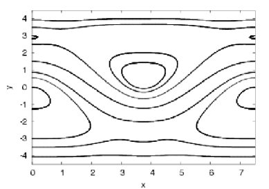
FIG. 1.: Stationary $(\epsilon=0)$ meandering jet streamlines.

The time dependence of the stream function is sufficient to produce Lagrangian chaos. The “chaoticity degree” is controlled by the two parameters $\epsilon$ and $\omega$. Specifically, there exists a threshold value $\epsilon_{c}(\omega)$ determining a transition from local to large-scale chaos, in agreement with Chirikov’s overlap of the resonances criterion [16, 17]. In the first case $(\epsilon<\epsilon_{c})$ chaos is confined to the stochastic layers around the separatrices, while in the second one $(\epsilon>\epsilon_{c})$ a large part of the phase space is visited by a chaotic trajectory, indicating the disappearance of any dynamical barriers to cross-stream transport [10]. In the plane $(\omega,\epsilon)$ the relation $\epsilon_{c}=\epsilon_{c}(\omega)$ defines a curve (Fig. 2) which separates regions with different dynamical properties, allowing one to discriminate between a nonoverlap (local chaos, i.e., chaos in a bounded region of $\Omega$) and an overlap (large scale-chaos) regime.

FIG. 2.: Overlap of the resonances: $\epsilon_{c}$ vs $\omega$. Here $\omega_{0}=0.25$ is the typical pulsation of recirculation.

In the following we will discuss transport in a non asymptotic situation, forcing the system to be in a small and closed basin, i.e., $0\leq x\leq 2\ell$. We use periodic boundary conditions along the $x$ axis; along the $y$ axis we set rigid boundary conditions in order to maintain trajectories in the strip $|y|<4$ even in the presence of a nonzero molecular diffusivity: particles reaching the horizontal lines $y=-4,4$ are reflected backward. We note here that, from a dynamical point of view, this system resembles the stratospheric polar vortex [2], once closed on itself in a circular geometry. This vortex models a current of isolated air in the high atmosphere, centered on the poles of the Earth, which has quite an important role in the dynamics of stratospheric ozone.

2 Stokes flow

This is a simple model of cellular flow, often used in the past because of its versatility, either from the experimental point of view or from the computational one [21, 22].
Its spatial structure in the stationary case is rather simple: there are only recirculation regions. Once periodic time dependence is switched on, stretching and folding of the streamlines can be seen and classic “coffee and cream” pathways take place. The flux is essentially driven from an upper ($V_{top}$) and a lower ($V_{bot}$) velocity; we choose to insert here time dependence in order to have Lagrangian chaos, setting $V_{top}=\cos{[\phi(t)]}$, $V_{bot}=\sin{[\phi(t)]}$. The stream function is

$$\psi(x,y,t)={1\over 2}\left\{(y+1)\cos[\phi(t)]+(y-1)\sin[\phi(t)]\right\}(1-x^{2})(1-y^{2})$$ (16)

where $\phi(t)=2\pi t/T$, and $T$ is the control parameter. At varying $T$ the dynamical properties of the system change from regular to chaotic. The first Lyapunov exponent reaches its maximum for $T$ comparable to the typical time of the unperturbed flow.

The constraint $V_{top}^{2}+V_{bot}^{2}=1$ can be looked at as a limited energy supply to the system.

Numerical results

We show here the numerical results for inert transport under the stirring of the above flows. In order to simulate more realistic dispersion processes, we integrate Eq.(5), including the effect of a nonzero molecular diffusivity $D_{0}$.

The study is carried out following the time evolution of a cloud of ${\mathcal{N}}\gg 1$ test particles, initially located in a small square of linear size $\delta_{\mbox{0}}\ll L$ (see Fig. 3).

           

           

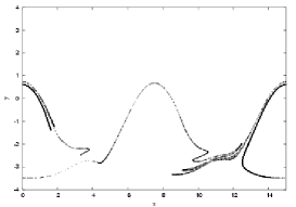
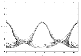
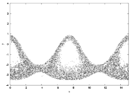
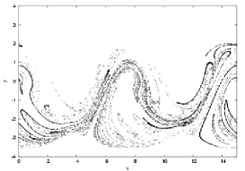
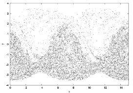
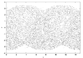
FIG. 3.: Meandering jet: dispersion of $10000$ particles at times (from the left to the right): $t=15,30,200$, in units of $T=2\pi/\omega=2\pi/0.625$ (perturbation’s period); top: $\epsilon=0.03$ (local chaos regime), bottom: $\epsilon=0.24$ (large-scale chaos regime).

We show the behavior of the two systems in the local chaos and large-scale chaos regime. We present mainly the result for the meandering jet; similar behaviors have been observed also in the Stokes flow. The role of the two different dynamical regimes is clearly seen in Fig. 4, where the fraction of occupied area is shown. The curves related to local chaos are always lower than the ones related to large-scale chaos, and the saturation times needed to invade the whole domain’s area are significantly different in the two cases.

For small values of the molecular diffusion coefficient, in the non overlap situation for system (15) it is possible to see a slowing down of the process, around half of the total area, due to the diffusive crossing of the jet. Let us incidentally note that, for $D_{0}=0$, no crossing of the jet would be possible for $\epsilon<\epsilon_{c}$. This can be seen in Fig. 3, where the dispersion of a cloud of test particles is plotted for the two dynamical regimes. Anyway, the presence of the noisy term (i.e., $D_{\mbox{0}}>0$) does not change the scenario if $D_{\mbox{0}}$ is small. See Fig. 4.

The differences in the saturation times progressively diminish for growing values of $D_{0}$ (left and right part of Fig. 4). Indeed, molecular diffusivity helps the dispersion process, acting itself as a mixing mechanism, though stochastic and not deterministic. For sufficiently large $D_{0}$ $[{\mathcal{O}}(10^{-2})$ - not shown here$]$, no difference is observable, due to the more relevant weight of the stochastic term with respect to the deterministic one in the Langevin equation (5).

     

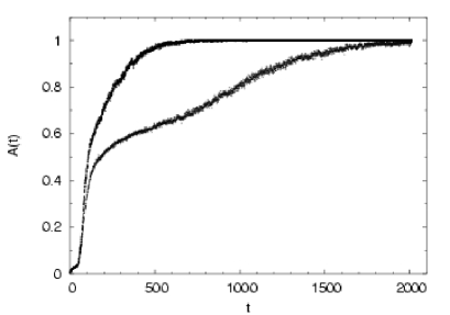
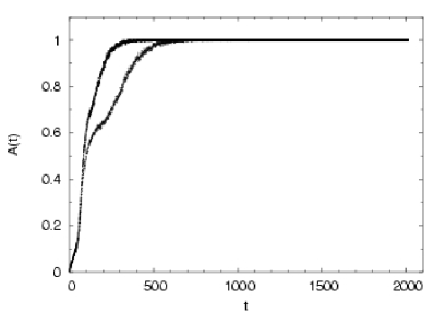
FIG. 4.: Meandering jet: occupied area vs $t$, on the left $D_{0}=0.001$, on the right $D_{0}=0.004$. Top curve shows the case with overlap of resonances $(\epsilon=0.24,\omega=0.625)$ (large scale chaos regime), bottom curve shows the case with nonoverlap of resonances $(\epsilon=0.03,\omega=0.625)$ (local chaos regime).

The behaviors of $t_{\alpha}$ as function of $t$ (Fig. 5) allow a more extensive analysis. With the same set of parameters as before, a wider scan in the values of chaos control parameters ($\epsilon$ for meandering jet, $T$ for Stokes flow) has been carried out for $\alpha=0.9$ and various values of $D_{0}$. As expected, these times slowly vary with the molecular diffusion coefficient in a strongly chaotic dynamical regime generated only by the flow. The dependence on $D_{0}$ becomes stronger when the dynamics only due to ${\mathbf{u}}$ is almost regular. In fact, our results show the great relevance of the details of the velocity field on mixing efficiency (see Fig. 5).

Moreover, we show mixing times for the Stokes flow together with an entropy graph. We plotted the quantity $c/h_{KS}$ versus $T$: $1/h_{KS}$ has dimensions of time and $c$ is a dimensionless parameter. Let us note that both $t_{\alpha}$ and $1/h_{KS}$ have minima for those values of $T$ which give the most chaotic dynamics.

We also remark that numerical values of our observables can depend on initial positions of test particles, but qualitative behaviors are general.

Let us observe that in the purely diffusive case (${\mathbf{u}}=0$) $t_{\alpha}$ is nothing but the ”bare” diffusive time needed to invade the whole domain. In that case we recovered the inverse proportionality relation $t_{\alpha}\sim L^{2}/D_{0}$.

     

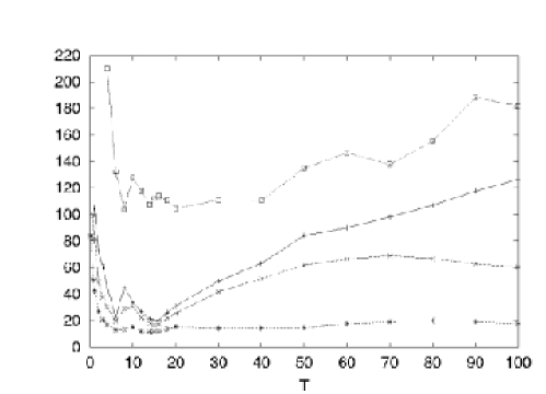
FIG. 5.: On the left, mixing times in the meandering jet: $t_{\alpha}$ vs $\epsilon$ at $\omega=0.625$. From the top to the bottom: $D_{\mbox{0}}=0.001,\>0.002,\>0.004$. On the right, Stokes flow: mixing times and inverse of Kolmogorov-Sinai entropy ($c/h_{KS}$) vs $T$. The time $c/h_{KS}$ (on top) is computed for $D_{0}=0$, mixing time curve are, from top to bottom $D_{\mbox{0}}=0.0005,\>0.001,\>0.004$.

III Reactive Case

Now we deal with the complete equation (1) studying an ARD system confined in a closed domain. As an initial condition we consider a small quantity of active material, i.e., $\theta=1$ in a small region of $\Omega$ with linear size $\delta_{\mbox{0}}$, elsewhere $\theta=0$. We numerically compute the time needed for a given percentage of the total area to be filled by the reaction (called, in the following, the reacting or burning time). A natural and important question is how the burning time depends on the transport properties of the flow.

The velocity fields are the already-presented meandering jet and Stokes flow. Our main result, obtained in both flows, is that the burning time is not strictly related to the transport properties of the flow.

As for the case of inert transport, the principal observable under investigation is the time needed for a given percentage of the total area to be burnt. We define

$$S(t)=\frac{1}{|\Omega|}\int_{\Omega}{\mathrm{d}}x{\mathrm{d}}y\theta(x,y,t),$$ (17)

as the percentage of area burnt at time $t$, where $|\Omega|$ is the area of the domain $\Omega$. In our case, we choose an appropriate localized initial condition such that the initial burnt material is $S(0)=0.005$. The reacting or burning time $t_{\alpha}$ is defined as the time needed for the percentage $\alpha$ of the total area of the recipient to be burnt, i.e.,

$$S(t_{\alpha})=\alpha\,\,.$$ (18)

           

           

FIG. 6.: Meandering jet ($2\ell$): Snapshots of the field $\theta(x,y,t)$ at times (from the left to the right): $t=4,5,7$, in units of $T=2\pi/\omega=2\pi/0.625$ (perturbation’s period); top row: $\epsilon=0.03$ (local chaos regime), bottom row $\epsilon=0.24$ (large-scale chaos regime); $D_{\mbox{0}}=0.001$. Black corresponds to $\theta=1$; white indicates $\theta=0$.

To numerically integrate Eq. (1) we followed a pseudo-Lagrangian approach. This algorithm uses a path integral formulation for $\theta(x,y,t)$: the field evolution is computed using the Lagrangian propagator plus a Monte Carlo integration for the diffusive term; then, the reaction propagator accounts for the reacting term (for details see Ref. [23]).

We impose a rigid wall condition in the boundaries, in order to avoid any fluid particle leaving the container, which could happen due to the noise term added to the velocity field in the Lagrangian approach.

Figure 6 shows some snapshots of the concentration field in the meandering jet flow for two different values of the control parameter. Comparing this figure with the analogous Fig. 3 in the inert case (using the same set of parameter), it is possible to have a clear insight of the different behavior of the system when reaction is present.

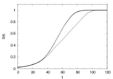
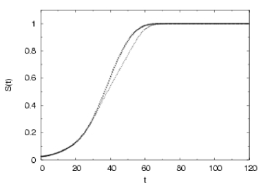
FIG. 7.: Meandering jet. Burnt area vs $t$, on the left $D_{\mbox{0}}=0.001$, on the right $D_{\mbox{0}}=0.004$, $\tau=2$, top curve $(\epsilon=0.24,\omega=0.625)$ (large-scale chaos regime), bottom curve $(\epsilon=0.03,\omega=0.625)$ (local chaos regime).

Figure 7, which shows the burnt area as a function of time in the case of local and large-scale chaos, has to be compared to the analogous Fig. 4 regarding the occupied area. It is apparent that, passing from local to large-scale chaotic dynamics, while the mixing efficiency changes greatly, the burning efficiency varies only slightly. This is a first evidence of the regularization properties of the reaction term. A further confirmation of such a feature comes from Fig. 8, where the burning efficiency is shown for different control parameters of the flows. In fact, it is possible to see that, at varying the control parameters, the burning efficiency changes only slightly. Such a behavior is very different from that observed for the mixing efficiency (see Fig. 5). Let us note that for the Stokes flow different values of the control parameter $T$ give similar mixing time, but different burning time (compare the right part of Figs. 5 and  8). Therefore, the burning efficiency is not so strictly related to the mixing properties of the flow. From Fig. 8 the presence of a plateau (and a consequent lower bound for the burning time) appears in the burning efficiency. As shown in Ref. [11] this plateau depends mainly on the reaction characteristic time.

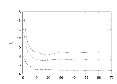
FIG. 8.: Burning times vs $t$. On the left meandering jet. $t_{\alpha}\>(\alpha=0.9)$ vs $\epsilon$, $\omega=0.625$ from the top to the bottom: $D_{\mbox{0}}=0.001,\>0.002,\>0.004$. On the right, Stokes flow. From top to bottom $D_{0}=\>0.0005,\>0.001,\>0.004$. In both cases the time scale of the chemistry is $\tau=2$.

The above results confirm the subtle and intriguing combined effect due to Lagrangian chaos, diffusion, and reaction. This issue is important to many different fields including the classical limit of quantum mechanics [14]. In Ref. [13] it is shown that, at variance with the inert transport [24], for the asymptotic front propagation properties, the role of the Lagrangian chaos is marginal if diffusion and reaction are present. In this preasymptotic problem we have that, independently of the details of ${\mathbf{u}}$ (in the presence or not of large-scale chaos) the dependence of $t_{\alpha}$ on $D_{\mbox{0}}$ is rather weak. In Fig. 9 we show $t_{\alpha}$ at varying $D_{0}$ in the plateau region for the Stokes flow and the meandering Jet. We have fair evidence that $t_{\alpha}\sim D_{\mbox{0}}^{-1/4}$, which is rather different from the result in absence of ${\mathbf{u}}$, i.e., $t_{\alpha}\sim L/v_{\mbox{f}}\sim D_{\mbox{0}}^{-1/2}$. In other words, in the reacting case, the combined effect of the advection reaction and diffusion allows an efficient non trivial “crossing of the dynamical barriers”.

FIG. 9.: Burning times vs $D_{\mbox{0}}$ for the meandering jet ($\circ$) and the Stokes flow ($\Box$) in the plateau region. The dotted lines show the behavior $t_{\alpha}\sim D_{\mbox{0}}^{-1/4}$; the dashed line shows the behavior $t_{\alpha}\sim D_{\mbox{0}}^{-1/2}$.

It is rather natural to wonder about the generality of the above results if one changes the term $f(\theta)$ using a non FKPP-type reaction term. The interesting case is when $f^{\prime}(0)=0$, for which the lower bound for the propagation velocity is 0. In this case, situations exist in which the presence of a velocity field can suppress front propagation [25]. However, if the reaction takes place in a closed domain, the reaction term is not pathological [we use the Arrhenius term $f(\theta)=(1-\theta)e^{-\theta_{c}/\theta}$] and the initial size of the active spot $\delta_{\mbox{0}}$ is not too small, the qualitative scenario showed above does not change. Figure 10 gives clear evidence of this.

FIG. 10.: Burning times for the meandering jet with an Arrhenius reaction term, $t_{\alpha}\>(\alpha=0.9)$ vs $\epsilon$, $\omega=0.625$ from the top to the bottom: $D_{\mbox{0}}=0.001,\>0.002,\>0.004$. The Arrhenius parameters are $\tau=2$ and $\theta_{c}=0.5$.

The behavior $t_{\alpha}\sim D_{\mbox{0}}^{-1/4}$ in the plateau region (see Fig. 9) is confirmed also in the Arrhenius case.

IV Conclusion

We have performed a numerical study of advection-reaction-diffusion systems confined in a closed domain and stirred by two different laminar velocities. Both the velocity fields can generate a regular or a chaotic Lagrangian dynamics, at varying control parameters. For the mixing properties of inert particles we observed that, when the dynamics is strongly chaotic, mixing times weakly depend on molecular diffusion; this feature becomes much more notable when the velocity field u is not strong enough to avoid the creation of recirculation regions.

Then, switching on the reaction term, we analyze the burning time of a reactive scalar in the same flows. The principal result of our study is that, while the mixing properties of the flows can change very much with varying dynamical properties, on the contrary the burning efficiency does not vary so much. We have also shown cases exist in which the burning efficiency is not strictly related to the mixing properties of the flows. Moreover, all the previous results are quite independent from the shape of the reaction term, $f(\theta)$.

We thank Massimo Cencini for a careful reading of the manuscript.

REFERENCES

-
[1]
E.R. Abraham, Nature 391, 577 (1998).
C. López, Z. Neufeld, E. Hernández-García and P.H. Haynes, Phys. Chem. Earth, B 26, 313 (2001). - [2] M. R. Schoeberl and D. L. Hartmann, Science, 251, 46 (1991).
-
[3]
Ya. B. Zeldovich and D.A. Frank-Kamenetskii,
Acta Physicochimica USSR, 9, 341-350 (1938).
N. Peters, Turbulent combustion, Cambridge University Press, Cambridge (2000). -
[4]
M. Leconte, J. Martin, N. Rakotomalala, and D. Salin,
Phys. Rev. Lett. 90, 128302 (2003).
M. S. Paoletti and T. H. Solomon, Europhys. Lett. 69, 819 (2005). -
[5]
A.N. Kolmogorov, I. Petrovskii and N. Piskunov,
Bull. Univ. Moscow, Ser. Int. A, 1, 1 (1937).
R.A. Fisher, Ann. Eugenics, 7, 353 (1937). -
[6]
J.D. Murray, Mathematical biology,
Springer-Verlag, Berlin (1993).
D.G. Aronson and H.F. Weinberger, Adv. Math., 30, 33 (1978). - [7] G. Boffetta, A. Celani, M. Cencini, G. Lacorata and A. Vulpiani, Chaos, 10, 50 (2000).
- [8] A. J. Majda, and P. R. Kramer, Phys. Rep., 314, 237 (1999).
- [9] P. Constantin, A. Kiselev, A. Oberman and L. Ryzhik, Arch. Rational Mechanics, 154, 53 (2000).
- [10] G. Boffetta, G. Lacorata, G. Redaelli and A. Vulpiani Physica, D 159, 59 (2001).
- [11] C. López, D. Vergni and A. Vulpiani, Eur. Phys. J. B 29, 117 (2002).
- [12] H. Aref. J. Fluid Mech. 143, 1 (1984).
- [13] M. Cencini, A. Torcini, D. Vergni and A. Vulpiani, Phys. of Fluids 15, 679 (2003).
- [14] M. Falcioni, A. Vulpiani, G. Mantica and S. Pigolotti, Phys. Rev. Lett. 91, 044101 (2003).
- [15] A. K. Pattanayak, Physica, D 148, 1 (2001).
- [16] B. V. Chirikov, Phys. Rep. 52, 263 (1979).
- [17] A. J. Lichtenberg and M. A. Lieberman, Regular and chaotic dynamics Springer-Verlag, 2nd edition (1993).
- [18] S. Cerbelli, A. Adrover and M. Giona, Phys. Lett. A 312, 355 (2003).
- [19] A. S. Bower, J. Phys. Oceanogr. 21, 173 (1991).
- [20] M. Cencini, G. Lacorata, A. Vulpiani and E. Zambianchi J. Phys. Oceanogr. 29, 2578 (1999).
- [21] A. Vikhansky, Phys. of Fluids 14, 2752 (2002).
- [22] C.W. Leong and J.M. Ottino, J. Fluid Mech. 209, 463 (1989).
- [23] M. Abel, A. Celani, D. Vergni and A. Vulpiani, Phys. Rev. E 64, 046307 (2001).
- [24] P. Castiglione, A. Mazzino, P. Muratore-Ginanneschi and A. Vulpiani, Physica D 134, 75 (1999).
- [25] N. Vladimirova, P. Constantin, A. Kiselev, O. Ruchayskiy and L. Ryzhik, Comb. Theory and Modelling, 154, 53 (2000).