The method of moments for Nonlinear Schrödinger Equations: Theory and Applications.

Abstract

The method of moments in the context of Nonlinear Schrödinger Equations relies on defining a set of integral quantities, which characterize the solution of this partial differential equation and whose evolution can be obtained from a set of ordinary differential equations. In this paper we find all cases in which the method of moments leads to closed evolution equations, thus extending and unifying previous works in the field of applications. For some cases in which the method fails to provide rigorous information we also develop approximate methods based on it, which allow to get some approximate information on the dynamics of the solutions of the Nonlinear Schrödinger equation.

1 Introduction

Nonlinear Schrödinger (NLS) equations appear in a great array of contexts [1] as for example in semiconductor electronics [2, 3], optics in nonlinear media [4], photonics [5], plasmas [6], fundamentation of quantum mechanics [7], dynamics of accelerators [8], mean-field theory of Bose-Einstein condensates [9] or in biomolecule dynamics [10]. In some of these fields and many others, the NLS equation appears as an asymptotic limit for a slowly varying dispersive wave envelope propagating in a nonlinear medium [11].

The study of these equations has served as the catalyzer of the development of new ideas or even mathematical concepts such as solitons [12] or singularities in EDPs [13, 14].

One of the most general ways to express a nonlinear Schrödinger equation, is

$$i\frac{\partial u}{\partial t}=-\frac{1}{2}\Delta u+V(x,t)u+g(|u|^{2},t)u-i\sigma(t)u$$ (1)

where $\Delta=\partial^{2}/\partial x_{1}^{2}+\cdots+\partial^{2}/\partial x_{n}^{2}$ and $u$ is a complex function which describes some physical wave. We shall consider here the solution of (1) on $\mathbb{R}^{n}$ and therefore $u:\mathbb{R}^{n}\times[0,T]\rightarrow\mathbb{C}$, with initial values $u(x,0)=u_{0}(x)\in X$, $X$ being an appropriate functional space ensuring finiteness of certain integral quantities to be defined later.

The family of nonlinear Schrödinger equations (1) contains many particular cases, depending on the specific choices of the nonlinear terms $g(|u|^{2},t)$, the potentials $V(x,t)$, the dissipation $\sigma(t)$ and the dimension of the space $n$. The best known cases are those of power-type $g(|u|^{2})=\alpha|u|^{p}$ or polinomial $g(|u|^{2})=\alpha_{1}|u|^{p_{1}}+\alpha_{2}|u|^{p_{2}}$ nonlinearities.

The potential term $V(x,t)$ models the action of an external force acting upon the system and may have many forms. Finally, we include in Eq. (1) a simple loss term arising in different applications [15, 16]. In many cases these losses are negligible, i. e. $\sigma=0$.

The description of the dynamics of initial data ruled by this equation is of great interest for applications. Nevertheless, gathering information about the solutions of a partial differential equation that is nonlinear like (1) constitutes a problem that is a priori nearly unapproachable. For this reason, most studies about the dynamics of this type of equation are exclusively numerical. The rigorous studies carried out to date concentrate on (i) properties of stationary solutions [17], (ii) particular results on the existence of solutions [18, 19], and (iii) asymptotic properties [13, 14].

Only when $n=1,g(\lvert u\rvert^{2},t)=\lvert u\rvert^{2},V(x,t)=0,\sigma=0$ it is possible to arrive at a solution of the initial value problem by using the inverse scattering transform method [12]. In this paper we develop the so-called method of moments, which tries to provide qualitative information about the behavior of the solutions of nonlinear Schrödinger equations. Instead of tackling the Cauchy problem (1) directly, the method studies the evolution of several integral quantities (the so-called moments) of the solution $u(x,t)$. In some cases the method allows to reduce the problem to the study of systems of coupled ordinary nonlinear differential equations. In other cases the method provides a foundation for making approximations in a more systematic (and simpler) way than other procedures used in physics, such as those involving finite-dimensional reductions of the original problem: namely the averaged Lagrangian, collective coordinates or variational methods [20, 21]. In any case the method of moments provides an information which is very useful for the applied scientist, who is usually interested in obtaining as much information as possible characterizing the dynamics of the solutions of the problem.

It seems that the first application of the method of moments was performed by Talanov [22] in order to find a formal condition of sufficiency for the blowup of solutions of the nonlinear Schrödinger equation with $g(|u|^{2})=-|u|^{2}$ and $n=2$. Since then, the method has been applied to different particular cases (mainly solutions of radial symmetry in two spatial dimensions), especially in the context of optics where many equations of NLS type arise [23].

In previous researchs, the method of moments has been studied in a range of specific situations but in all the cases the success of the method is unrelated to a more general study. In this paper we try to consider the method systematically and solve a number of open questions: (i) to find the most general type of nonlinear term and potentials in Eq. (1) for which the method of moments allows to get conclusions and (ii) to develop approximate methods based on it for situations in which the moment equations do not allow to obtain exact results.

2 Preliminary considerations

Let us define the functional space $Q(H)$ as the space of functions for which the so called energy functional

$$E(u)=(u,Hu)_{L^{2}(\mathbb{R}^{n})}+\int_{\mathbb{R}^{n}}G(|u|^{2},t)dx$$ (2)

is finite, $G$ being a function such that $\partial G(|u|^{2},t)/\partial|u|^{2}=g(|u|^{2},t)$, $(\cdot,\cdot)_{L^{2}(\mathbb{R}^{n})}$ denoting the usual scalar product in $L^{2}(\mathbb{R}^{n})$ and $H=-\frac{1}{2}\Delta+V(x,t)$. For the case $V(x,t)=0$ and $g$ independent of time, several results on existence and unicity were given by Ginibre and Velo [18].

As regards the case $V\neq 0$, which is the one we are mainly interested in our work, the best documented case in the literature is that of potentials with $|D^{\alpha}V|$ bounded in $\mathbb{R}^{n}$ for every $|\alpha|\geq 2$; that is, potentials with at most quadratic growth. Y. Oh [24] proved the local existence of solutions in $L^{2}(\mathbb{R}^{n})$ and in $Q(H)$ for nonlinearities of the type $g(u)=-|u|^{p},0\leq p<4/n$. However the procedure used allows to substitute this nonlinearity with other more general ones. It seems also posible to extend the results to the case in which the potential depends on $t$.

Therefore, from now on we shall suppose that the nonlinear term satisfies the conditions set by Ginibre and Velo and that $|D^{\alpha}V|$ is bounded in space for all $|\alpha|\geq 2$. Under these conditions it is posible to guarantee at least local existence of solutions of Eq. (1) in appropriate functional spaces.

2.1 Formal elimination of the loss term

In the first place we carry out the transformation [15]

$$\hat{u}(x,t)=u(x,t)e^{\int_{0}^{t}\sigma(\tau)d\tau},$$ (3)

which is well defined for any bounded function $\sigma(t)$ (this includes all known realistic cases arising in the applications). The equation satisfied by $\hat{u}(x,t)$ is obtained from the following direct calculation:

$$i\frac{\partial\hat{u}}{\partial t} = i\frac{\partial u}{\partial t}e^{\int_{0}^{t}\sigma(\tau)d\tau}+i\sigma(t)ue^{\int_{0}^{t}\sigma(\tau)d\tau}$$

$$= \left[-\frac{1}{2}\Delta u+V(x,t)u+g(|u|^{2},t)u-i\sigma(t)u\right]e^{\int_{0}^{t}\sigma(\tau)d\tau}+i\sigma(t)ue^{\int_{0}^{t}\sigma(\tau)d\tau}$$

$$= -\frac{1}{2}\Delta\hat{u}+V(x,t)\hat{u}+\hat{g}(|\hat{u}|^{2},t)\hat{u}$$

where

$$\hat{g}(|\hat{u}|^{2},t)=g(|u|^{2},t)=g(e^{-2\int_{0}^{t}\sigma(\tau)d\tau}|\hat{u}|^{2},t).$$ (4)

From here on we shall consider, with no loss of generality, that $\sigma(t)=0$ in Eq. (1) assuming that this choice might add an extra time-dependence to the nonlinear term.

3 The method of moments: Generalities

3.1 Definition of the moments

Let us define the following quantities:

$$I_{k,j}(t) = \int x_{j}^{k}|u(x,t)|^{2}dx=\left\|x_{j}^{k/2}u\right\|^{2}_{L^{2}(\mathbb{R}^{n})},$$ (5a)

$$V_{k,j}(t) = 2^{k-1}i\int x_{j}^{k}\left(u(x,t)\frac{\partial\bar{u(x,t)}}{\partial x_{j}}-\bar{u}\frac{\partial u(x,t)}{\partial x_{j}}\right)dx,$$ (5b)

$$K_{j}(t) = \frac{1}{2}\int\left|\frac{\partial u(x,t)}{\partial x_{j}}\right|^{2}dx=\frac{1}{2}\left\|\frac{\partial u}{\partial x_{j}}\right\|^{2}_{L^{2}(\mathbb{R}^{n})}$$ (5c)

$$J(t) = \int G(|u(x,t)|^{2},t)dx,$$ (5d)

with $j=1,...,n$ and $k=0,1,2,...$, which we will call moments of $u(x,t)$ in analogy with the moments of a distribution. From now on and also in Eqs. (5) it is understood that all integrals and norms refer to the spatial variables $x\in\mathbb{R}^{n}$ unless otherwise stated. In Eqs. (5) we denote by $\bar{u}$ the complex conjugate of $u$.

In some cases we will make specific reference to which solution $u$ of Eq. (1) is used to calculate the moments by means of the notation: $I^{u}_{k,j}$, etc.

The moments are quantities that have to do with intuitive properties of the solution $u(x,t)$. For example, the moment $I_{0,0}$ is the squared $L^{2}(\mathbb{R}^{n})$-norm of the solution and therefore measures the magnitude, quantity or mass thereof. Depending on the particular context of application, this moment is denominated mass, charge, intensity, energy, number of particles, etc. The moments $I_{1,j}(t)$ are the coordinates of the center of the distribution $u$, giving us an idea of the overall position thereof. The quantities $I_{2,j}$ are related with the width of the distribution defined as $W_{j}=(\int_{\mathbb{R}^{n}}(x_{j}-I_{1,j})^{2}|u|^{2}dx)^{1/2}=(I_{2,j}+I_{1,j}^{2}I_{0,0}-2I_{1,j}^{2})^{1/2}$, which is also a quantity with an evident meaning.

The evolution of the moments is determined by that of the function $u(x,t)$. From now on we will assume that the initial datum $u_{0}(x)$ and the properties of the equation guarantee that the moments are well defined for all time.

3.2 First conservation law

It is easy to prove formally that the moment $I_{0,0}$ is invariant during the temporal evolution by just calculating

$$\frac{d}{dt}I_{0,0}(t) = \int_{\mathbb{R}^{n}}\left(\frac{d}{dt}|u|^{2}\right)dx=\int_{\mathbb{R}^{n}}\left(\bar{u}\frac{\partial}{\partial t}u+u\frac{\partial}{\partial t}\bar{u}\right)dx$$ (6)

$$= \int_{\mathbb{R}^{n}}i\left(\frac{1}{2}\bar{u}\Delta u-V(x,t)|u|^{2}-g(|u|^{2},t)|u|^{2}\right)dx$$

$$+\int_{\mathbb{R}^{n}}i\left(-\frac{1}{2}u\Delta\bar{u}+V(x,t)|u|^{2}+g(|u|^{2},t)|u|^{2}\right)dx$$

$$= \int_{\mathbb{R}^{n}}\frac{i}{2}\left(\bar{u}\Delta u-u\Delta\bar{u}\right)dx$$

$$= \frac{i}{2}\left(\int_{\mathbb{R}^{n}}|\nabla u|^{2}dx-\int_{\mathbb{R}^{n}}|\nabla u|^{2}dx\right)=0,$$

where we have performed integration by parts and used that the function $u$ and its derivatives vanish at infinity.

Obviously the above demonstration is formal in the sense that a regularity which we do not know for certain has been used for $u$. Nevertheless, this type of proof can be formalized by making a convolution of the function $u$ with a regularizing function. The details of these methodologies can be seen in [18] or [24]. In this paper we will limit ourselves to formal calculations.

4 General results for harmonic potentials

4.1 Introduction

From this point onward we will focus on the particular case of interest for this study when $V(x,t)$ is a harmonic potential of the type $V(x,t)=\frac{1}{2}(x,\Lambda(t)x)$, where $\Lambda$ is a real matrix of the form $\Lambda_{ij}(t)=\lambda_{i}^{2}(t)\delta_{ij}$, with $\lambda_{i}\geq 0$ for $i=1,...,n$ and $\delta_{ij}$ is the Kronecker delta. Bearing in mind the results of Section 2.1, the NLS equation under study is then

$$i\frac{\partial u}{\partial t}=-\frac{1}{2}\Delta u+\frac{1}{2}\left(\sum_{j=1}^{n}\lambda_{j}^{2}x_{j}^{2}\right)u+g(|u|^{2},t)u.$$ (7)

This equation appears in a wide variety of applications such as propagation of waves optical transmission lines with online modulators [26, 27, 28, 29], propagation of light beams in nonlinear media with a gradient of the refraction index [30, 31], or dynamics of Bose-Einstein condensates [9]. Generically it can provide a model for studying some properties of the solutions of nonlinear Schrödinger equations localized near a minimum of a general potential $V(x)$.

4.2 First moment equations

If we differentiate the definitions of the moments $I_{1,j}$ and $V_{0,j}$, we obtain, after some calculations, the evolution equations

$$\frac{dI_{1,j}}{dt} = V_{0,j},$$ (8a)

$$\frac{dV_{0,j}}{dt} = -\lambda_{j}^{2}I_{1,j},$$ (8b)

so that $I_{1,j},j=1,...,n$ satisfy

$$\frac{d^{2}I_{1,j}}{dt^{2}}+\lambda_{j}^{2}I_{1,j}=0$$ (9)

with inital data $I_{1,j}(0),\dot{I}_{1,j}(0)=V_{0,j}(0)$. These expressions are a generalization of the Ehrenfest theorem of linear quantum mechanics to the nonlinear Schrödinger equation and particularized for the potential that concerns us [24, 32].

This result has been discussed previously in many papers and is physically very interesting. It indicates that the evolution of the center of the solution is independent of the nonlinear effects and of the evolution of the rest of the moments and depends only on the potential parameters.

4.3 Reduction of the general problem to the case $\boldsymbol{I_{1,j}=V_{0,j}=0}$

We shall begin by stating the following lemma [33]:

Lemma 1.

Let $u(x,t)$ be a solution of (7) with the initial datum $u(x,0)=u_{0}(x)$. Then, the functions

$$u_{R}(x,t)=u(x-R(t),t)e^{i\theta(x,t)}$$ (10a)

where

$$\theta(x,t)=\left(x,\dot{R}\right)+\int_{0}^{t}\left[(\dot{R}(t^{\prime}),\dot{R}(t^{\prime}))-(R(t^{\prime}),\Lambda(t^{\prime})R(t^{\prime}))\right]dt^{\prime}$$ (10b)

and

$$\frac{d^{2}R}{dt^{2}}+\Lambda R=0$$ (10c)

for any set of initial data $$R(0),\dot{R}(0)\in\mathbb{R}^{n}$$ are also solutions of (7).

Proof.

All we have to do is substitute (10a), (10b) and (10c) in (7). ∎

One noteworthy conclusion is that given a solution of Eq. (7) we can translate it initially by a constant vector and obtain another solution. In the case of stationary states, defined as solutions of the form

$$u(x,t)=\varphi_{\mu}(x)e^{i\mu t}$$ (11)

which exist in the autonomous case (i.e. $d\lambda/dt=0$) and whose dynamics are trivial, this result implies that under displacements the only dynamics acquired are those of the movement of the center given by Eq. (10c). The coincidence of the evolution laws (9) and (10c) allows us to state the following theorem which is an immediate consequence of the above lemma.

Theorem 2.

If $\psi(x,t)$ is a solution of (7) with non-zero $I^{\psi}_{1,j}$ or $V^{\psi}_{0,j}$, then there exists a unique solution $u(x,t)=\psi(x+\{I^{\psi}_{1,j}(t)\}_{j},t)e^{i\theta(x,t)}$ with

$$\theta(x,t)=-\sum_{j}x_{j}V^{\psi}_{0,j}+\sum_{j}\left[\int_{0}^{t}V^{\psi}_{0,j}(t^{\prime})^{2}-\lambda_{j}(t^{\prime})^{2}I_{1,j}^{\psi}(t^{\prime})^{2}\right]dt^{\prime}$$

such that $I^{u}_{1,j}=0$ and $V^{u}_{0,j}=0$

The important conclusion of this theorem is that it suffices to study solutions with $I_{1,j}$ and $V_{0,j}$ equal to zero, as those that have one of these coefficients different from zero can be obtained from previous ones, by means of translation and multiplication by a linear phase in $x$. From a practical standpoint, what is most important is that $I_{1,j}$ be null without any loss of generality, as then we can establish a direct link between the widths and the moments $I_{2,j}$ (see the discussion in the third paragraph of Section 3).

4.4 Moment Equations

Assuming that all of the moments can be defined at any time $t$, we can calculate their evolution equations by means of direct differentiation. The results are gathered in the next theorem.

Theorem 3.

Let $u_{0}(x)$ be an initial datum such that the moments $I_{2,j},V_{1,j},K_{j}$ and $J$ are well defined at $t=0$. Then

$$\frac{dI_{2,j}}{dt} = V_{1,j},$$ (12a)

$$\frac{dV_{1,j}}{dt} = 4K_{j}-2\lambda_{j}^{2}I_{2,j}-2\int_{\mathbb{R}^{n}}D(\rho,t)dx,$$ (12b)

$$\frac{dK_{j}}{dt} = -\frac{1}{2}\lambda_{j}^{2}V_{1,j}-\int_{\mathbb{R}^{n}}D(\rho,t)\frac{\partial^{2}\phi}{\partial x_{j}^{2}}\,dx,$$ (12c)

$$\frac{dJ}{dt} = \int_{\mathbb{R}^{n}}D(\rho,t)\Delta\phi\,dx+\int_{\mathbb{R}^{n}}\frac{\partial G(\rho,t)}{\partial t}dx.$$ (12d)

where $D(\rho,t)=G(\rho,t)-\rho g(\rho,t)$, $\rho=|u(x,t)|^{2}$.

Proof.

The demonstration of the validity of Eqs. (12) can be carried out from direct calculations, performing integration by parts, and using the decay of $u$ and $\nabla u$ at infinity.

To demonstrate (12a) it is easier to work with the modulus-phase representation of $u$, $u=\rho^{1/2}e^{i\phi}$ (with $\rho>0$). Then

$$\frac{dI_{2,j}}{dt} = \int x_{j}^{2}\dot{\rho}=-\int x_{j}^{2}(\nabla\rho\cdot\nabla\phi+\rho\Delta\cdot\phi)$$

$$= -\int x_{j}^{2}\nabla\rho\cdot\nabla\phi+\int\nabla(x_{j}^{2}\rho)\cdot\nabla\phi$$

$$= -\int x_{j}^{2}\nabla\rho\cdot\nabla\phi+\int x_{j}^{2}\nabla\rho\cdot\nabla\phi+\int\nabla(x_{j}^{2})\rho\cdot\nabla\phi$$

$$= 2\int x_{j}\rho\frac{\partial\phi}{\partial x_{j}}=V_{1,j}.$$

We can also prove (12b) as follows

$$\frac{dV_{1,j}}{dt} = i\int x_{j}\left(u_{t}\frac{\partial\bar{u}}{\partial x_{j}}+u\frac{\partial\bar{u_{t}}}{\partial x_{j}}-\bar{u_{t}}\frac{\partial u}{\partial x_{j}}-\bar{u}\frac{\partial u_{t}}{\partial x_{j}}\right)$$ (13)

$$= \int x_{j}\left[-\frac{1}{2}\Delta u\frac{\partial\bar{u}}{\partial x_{j}}+\frac{1}{2}\left(\sum\lambda_{k}^{2}x_{k}^{2}\right)u\frac{\partial\bar{u}}{\partial x_{j}}+gu\frac{\partial\bar{u}}{\partial x_{j}}+u\frac{1}{2}\frac{\partial\Delta\bar{u}}{\partial x_{j}}\right.$$

$$\left.-\lambda_{j}^{2}x_{j}|u|^{2}-\frac{1}{2}\left(\sum\lambda_{k}^{2}x_{k}^{2}\right)u\frac{\partial\bar{u}}{\partial x_{j}}-\frac{\partial g}{\partial x_{j}}|u|^{2}-gu\frac{\partial\bar{u}}{\partial x_{j}}+\mbox{c.c.}\right]$$

$$= -2\lambda_{j}^{2}\int x_{j}^{2}|u|^{2}-2\int x_{j}|u|^{2}\frac{\partial g}{\partial x_{j}}$$

$$-\frac{1}{2}\int x_{j}\left(\Delta u\frac{\partial\bar{u}}{\partial x_{j}}+\Delta\bar{u}\frac{\partial u}{\partial x_{j}}-u\frac{\partial\Delta\bar{u}}{\partial x_{j}}+\bar{u}\frac{\partial\Delta u}{\partial x_{j}}\right),$$

where c.c. indicates the complex conjugate. Operating on the above integrals we have

$$\int x_{j}\left(\Delta u\frac{\partial\bar{u}}{\partial x_{j}}+\Delta\bar{u}\frac{\partial u}{\partial x_{j}}-u\frac{\partial\Delta\bar{u}}{\partial x_{j}}-\bar{u}\frac{\partial\Delta u}{\partial x_{j}}\right)$$

$$=-2\int x_{j}\left(\nabla u\cdot\frac{\partial\nabla\bar{u}}{\partial x_{j}}+\nabla\bar{u}\cdot\frac{\partial\nabla u}{\partial x_{j}}\right)-4\int\left|\frac{\partial u}{\partial x_{j}}\right|^{2}-2\int|\nabla u|^{2}$$

$$=2\int|\nabla u|^{2}-4\int\left|\frac{\partial u}{\partial x_{j}}\right|^{2}-2\int|\nabla u|^{2}=-4\int\left|\frac{\partial u}{\partial x_{j}}\right|^{2},$$

and

$$\int x_{j}\frac{\partial g}{\partial x_{j}}\rho=-\int g\rho-\int x_{j}\frac{\partial G}{\partial x_{j}}=-\int g\rho+\int G=\int D.$$

By substitution in (13) we arrive at the desired result.

$$\frac{dV_{1,j}}{dt} = -2\lambda_{j}^{2}\int x_{j}^{2}|u|^{2}+2\int\left|\frac{\partial u}{\partial x_{j}}\right|^{2}-2\int D$$

$$= -2\lambda_{j}^{2}I_{2,j}+4K_{j}-2\int D.$$

Let us now prove (12c)

$$\frac{dK_{j}}{dt} = \frac{1}{2}\int\frac{d}{dt}\left(\frac{\partial u}{\partial x_{j}}\frac{\partial\bar{u}}{\partial x_{j}}\right)=\frac{1}{2}\int\left(\frac{\partial u_{t}}{\partial x_{j}}\frac{\partial\bar{u}}{\partial x_{j}}+\frac{\partial u}{\partial x_{j}}\frac{\partial\bar{u_{t}}}{\partial x_{j}}\right)$$

$$= \frac{1}{2}\int\frac{\partial}{\partial x_{j}}\left[\frac{i}{2}\Delta u-\frac{i}{2}\left(\sum_{k=1}^{n}\lambda_{k}^{2}x_{k}^{2}\right)u-igu\right]\frac{\partial\bar{u}}{\partial x_{j}}+\mbox{c.c.},$$

then

$$\frac{dK_{j}}{dt} = -\frac{i}{2}\lambda_{j}^{2}\int x_{j}\left(u\frac{\partial\bar{u}}{\partial x_{j}}-\bar{u}\frac{\partial u}{\partial x_{j}}\right)-\frac{i}{2}\int\frac{\partial g}{\partial x_{j}}\left(u\frac{\partial\bar{u}}{\partial x_{j}}-\bar{u}\frac{\partial u}{\partial x_{j}}\right)$$

$$+\frac{i}{4}\int\left(\frac{\partial\Delta u}{\partial x_{j}}\frac{\partial\bar{u}}{\partial x_{j}}-\frac{\partial u}{\partial x_{j}}\frac{\partial\Delta\bar{u}}{\partial x_{j}}\right)=-\frac{1}{2}\lambda_{j}^{2}V_{1,j}+\int g\frac{\partial}{\partial x_{j}}\left(\rho\frac{\partial\phi}{\partial x_{j}}\right)$$

$$= -\frac{1}{2}\lambda_{j}^{2}V_{1,j}+\int g\left(\rho\frac{\partial^{2}\phi}{\partial x_{j}^{2}}+\frac{\partial\rho}{\partial x_{j}}\frac{\partial\phi}{\partial x_{j}}\right),$$

and using the definition of $G$ we obtain

$$\frac{dK_{j}}{dt} = -\frac{1}{2}\lambda_{j}^{2}V_{1,j}+\int g\rho\frac{\partial^{2}\phi}{\partial x_{j}^{2}}+\int\frac{\partial G}{\partial x_{j}}\frac{\partial\phi}{\partial x_{j}}$$

$$= -\frac{1}{2}\lambda_{j}^{2}V_{1,j}+\int g\rho\frac{\partial^{2}\phi}{\partial x_{j}^{2}}-\int G\frac{\partial^{2}\phi}{\partial x_{j}^{2}}$$

$$= -\frac{1}{2}\lambda_{j}^{2}V_{1,j}-\int(G-\rho g)\frac{\partial^{2}\phi}{\partial x_{j}^{2}}=-\frac{1}{2}\lambda_{j}^{2}V_{1,j}-\int D\frac{\partial^{2}\phi}{\partial x_{j}^{2}}.$$

Finally, to demonstrate (12d) we proceed

$$\frac{dJ}{dt} = \int\frac{dG(\rho,t)}{dt}=\int\left[\frac{\partial G}{\partial\rho}\left(\frac{\partial\rho}{\partial u}u_{t}+\frac{\partial\rho}{\partial\bar{u}}\bar{u}_{t}\right)+\frac{\partial G}{\partial t}\right]$$

$$= \int\left[\frac{\partial G}{\partial\rho}\left(\bar{u}u_{t}+u\bar{u}_{t}\right)+\frac{\partial G}{\partial t}\right]=\frac{i}{2}\int\left[g\left(\bar{u}\Delta u-u\Delta\bar{u}\right)+\frac{\partial G}{\partial t}\right]$$

$$= \int\left[-g\nabla\cdot(\rho\nabla\phi)+\frac{\partial G}{\partial t}\right]=\int\left[-g\nabla\rho\cdot\nabla\phi-g\rho\Delta\phi+\frac{\partial G}{\partial t}\right]$$

$$= \int\left[-\nabla G\cdot\nabla\phi-g\rho\Delta\phi+\frac{\partial G}{\partial t}\right]=\int\left(G-g\rho\right)\Delta\phi+\int\frac{\partial G}{\partial t}$$

$$= \int D\Delta\phi+\int\frac{\partial G}{\partial t}.$$

∎

A direct consequence of the theorem is

Corollary 4.

Let $u(x,t)$ be a stationary solution of (7). Then,

$$K_{j}=\frac{1}{2}\lambda_{j}^{2}I_{2,j}+\frac{1}{2}\int D(\rho)dx.$$ (14)

5 Solvable cases of the method of moments

In this section we will study several particular situations of practical relevance in which the method of moments thoroughly provides exact results.

5.1 The linear case $\boldsymbol{g(\rho,t)=0}$

In this case, Eqs. (5d) and (12d) tells us that $J(t)=0$, for all $t$, and then the moment equations (12) become

$$\frac{dI_{2,j}}{dt} = V_{1,j},$$ (15a)

$$\frac{dV_{1,j}}{dt} = 4K_{j}-2\lambda_{j}^{2}I_{2,j},$$ (15b)

$$\frac{dK_{j}}{dt} = -\frac{1}{2}\lambda_{j}^{2}V_{1,j}.$$ (15c)

That is, in the linear case the equations for the moments along each direction $j$ of the physical space $\mathbb{R}^{n}$ are uncoupled. This property was known in the context of optics for $n=2$ and constant $\lambda_{j}$ [34]. Here we see that this property holds for any number of spatial dimensions, time dependence $\lambda(t)$ and even for nonsymmetric initial data.

5.2 Condition of closure of the moment equations in the general case

Equations (12) do not form a closed set and therefore to obtain, in general, their evolution we would need to continue obtaining moments of a higher order, which would provide us with an infinite hierarchy of differential equations. Given the similarity among the terms that involve second derivatives of the phase of the solution in Eqs. (12), it is natural to wonder whether it would be possible to somehow close the system and thus obtain information about the solutions.

From this point on, and for the rest of the section, we will limit ourselves to the case $\lambda_{j}(t)=\lambda(t),j=1,\ldots,n$, which is the most realistic one, and which includes as a particular case the situation without external potentials $\lambda_{j}=0$. Let us define the following quantities

$$\mathcal{I}=\sum_{j=1}^{n}I_{2,j},\ \mathcal{V}=\sum_{j=1}^{n}V_{1,j},\ \mathcal{K}=\sum_{j=1}^{n}K_{j}.$$ (16)

Differentiating equations (16) and using (12), we have

$$\frac{d\mathcal{I}}{dt} = \mathcal{V},$$ (17a)

$$\frac{d\mathcal{V}}{dt} = 4\mathcal{K}-2\lambda^{2}\mathcal{I}-2n\int_{\mathbb{R}^{n}}D(\rho,t)dx,$$ (17b)

$$\frac{d\mathcal{K}}{dt} = -\frac{1}{2}\lambda^{2}\mathcal{V}-\int_{\mathbb{R}^{n}}D(\rho,t)\Delta\phi dx,$$ (17c)

$$\frac{dJ}{dt} = \int_{\mathbb{R}^{n}}D(\rho,t)\Delta\phi+\int_{\mathbb{R}^{n}}\frac{\partial G(\rho,t)}{\partial t}dx.$$ (17d)

If we add up equations (17c) and (17d) we arrive at

$$\frac{d\mathcal{I}}{dt} = \mathcal{V},$$ (18a)

$$\frac{d\mathcal{V}}{dt} = 4\left[\mathcal{K}-\frac{n}{2}\int_{\mathbb{R}^{n}}D(\rho,t)dx\right]-2\lambda^{2}\mathcal{I},$$ (18b)

$$\frac{d\left(\mathcal{K}+J\right)}{dt} = -\frac{1}{2}\lambda^{2}\mathcal{V}+\int_{\mathbb{R}^{n}}\frac{\partial G}{\partial t}dx.$$ (18c)

In order that equations (18) form a closed system, they must fulfill that $-\tfrac{n}{2}\int_{\mathbb{R}^{n}}D(\rho,t)dx=J=\int_{\mathbb{R}^{n}}G(\rho,t)dx$ and that $\int_{\mathbb{R}^{n}}\frac{\partial G(\rho,t)}{\partial t}dx$ can be expressed in terms of the other known quantities. The former condition requires that

$$0=\int_{\mathbb{R}^{n}}\left[\frac{n}{2}D(\rho,t)+G(\rho,t)\right]dx=\int_{\mathbb{R}^{n}}\left[\left(1+\frac{n}{2}\right)G(\rho,t)-\frac{n}{2}\frac{\partial G(\rho,t}{\partial\rho}\rho\right]dx.$$

As $G(\rho,t)$ does not depend explicitly on $x$, this condition is verified when

$$\frac{\partial G(\rho,t)}{\partial\rho}=\left(1+\frac{2}{n}\right)\frac{G(\rho,t)}{\rho},$$ (19)

that is, if

$$G(\rho,t)=g_{0}(t)\rho^{1+2/n},$$ (20)

or, equivalently, if

$$g(\rho,t)=g_{0}(t)\rho^{2/n},$$ (21)

where $g_{0}(t)$ is an arbitrary function that indicates the temporal variation of the nonlinear term. Then

$$\int_{\mathbb{R}^{n}}\frac{\partial G(\rho,t)}{\partial t}dx=\frac{1}{g_{0}}\frac{dg_{0}}{dt}\int_{\mathbb{R}^{n}}G(\rho,t)dx=\frac{1}{g_{0}}\frac{dg_{0}}{dt}J(t).$$ (22)

To close the equations it is necessary that $g_{0}(t)$ be constant in order to cancel the last term of this expression. Then, the nonlinearities for which it is possible to find closed results are

$$g(\rho)=g_{0}\rho^{2/n}=g_{0}|u|^{4/n},$$ (23)

with $g_{0}\in\mathbb{R}$, remembering that in the case $g_{0}<0$ there may be problems of blowup in finite time. Fortunately, these nonlinearities for $n=1,2,3$ correspond to cases of practical interest. For instance, the case $n=1$ with quintic nonlinearity has been studied in Refs. [35, 36, 37] and the case $n=2$, with cubic nonlinearity, corresponds probably to the most relevant instance of NLS equation, i.e. the cubic one in two spatial dimensions [30, 31]. For $n=3$ the nonlinearity given by Eq. (23) appears in the context of the Hartree-Fock theory of atoms.

5.3 Simplification of the moment equations

Defining a new quantity $\mathcal{E}=\mathcal{K}+J$, Eqs. (18) become

$$\frac{d\mathcal{I}}{dt} = \mathcal{V},$$ (24a)

$$\frac{d\mathcal{V}}{dt} = 4\mathcal{E}-2\lambda^{2}(t)\mathcal{I},$$ (24b)

$$\frac{d\mathcal{E}}{dt} = -\frac{1}{2}\lambda^{2}(t)\mathcal{V}.$$ (24c)

These equations form a set of non-autonomous linear equations for the three averaged moments: $\mathcal{E}(t),\mathcal{V}(t)$ and $\mathcal{I}(t)$. To continue our analysis, we note that

$$\mathcal{Q}=2\mathcal{E}\mathcal{I}-\frac{1}{4}\mathcal{V}^{2},$$ (25)

is a dynamical invariant of Eqs. (24). We finally define $X=\left|\mathcal{Q}\right|^{-1/4}\mathcal{I}^{1/2}$, which is proportional to the mean width of $u$. A simple calculation allows us to corroborate that the equation that $X(t)$ satisfies is

$$\frac{d^{2}X}{dt^{2}}+\lambda^{2}(t)X=\frac{\text{sgn}(\mathcal{Q})}{X^{3}}.$$ (26)

Solving (26) allows to calculate $\mathcal{V}$ and $\mathcal{E}$ by simple substitution in (24). This equation is similar to that obtained in [30] for solutions of radial symmetry in the case $n=2$ and $g(u)=|u|^{2}$. Here we find that it is possible to obtain a more general result for solutions without specific symmetry requirements, and for any combination of dimension and nonlinearity $g(u)=|u|^{p}$ satisfying the condition $np=4$. The case with $\text{sgn}(\mathcal{Q})=-1$ corresponds to collapsing situations [13, 38]. In what follows we consider mostly the case $\mathcal{Q}>0$.

Equation (26) was studied by Ermakov in 1880 [39], although since then it has been rediscovered many times (see e.g. [40]). It is a particular case of the so-called Ermakov systems [41, 42, 43], for which it is possible to give fairly complete results. Especially easy, though tedious to demonstrate is

Theorem 5 (Ermakov, 1880).

Let $X(t)$ be the solution of (26) with initial data $X(0)=X_{0},\dot{X}(0)=\dot{X}_{0}$. Then, if $\chi_{1}(t)$ and $\chi_{2}(t)$ are solutions of the differential equation

$$\frac{d^{2}\chi}{dt^{2}}+\lambda^{2}(t)\chi=0$$ (27a)

satisfying the initial data $$\chi_{1}(0)=X_{0},\dot{\chi}_{1}(0)=\dot{X}_{0} \chi_{2}(0)=0,\dot{\chi}_{2}(0)\neq 0$$ and then

$$X(t)=\sqrt{\chi^{2}_{1}(t)+\frac{1}{w^{2}}\chi_{2}^{2}(t)}$$ (27b)

where $w$ is the constant $w=\chi_{1}\dot{\chi}_{2}-\chi_{2}\dot{\chi}_{1}$.

Equation (27b) is often called the principle of nonlinear superposition. Equation (27a) is the well known Hill’s equation [44] which modelizes a parametrically forced oscillator, and which has been studied in depth. In the following, we shall study a couple of special situations in view of their physical interest.

It is remarkable that the complex dynamics of a family of nonlinear partial differential equations can be understood in terms of a simple equation such as Hill’s.

If we suppose that the function $\lambda^{2}(t)$ depends on a parameter $\varepsilon$ in the way $\lambda^{2}(t)=1+\tilde{\lambda}_{\varepsilon}(t)$, $\tilde{\lambda}_{\varepsilon}(t)$ being a periodic function with maximum value $\varepsilon$ (not necessarily small), there exists a complete theory that describes the intervals of values of $\varepsilon$ for which the solutions of Eq. (27a) are bounded (intervals of stability) and the intervals for which the solutions are unbounded (intervals of instability) [44].

6 Applications

6.1 Dynamics of laser beams in GRIN media

When a laser beam propagates in a medium with a gradex refraction index (GRIN medium) with an specific profile quadratic in the transverse coordinates, the distribution of intensity $u(x,y,z)$ in permanent regime is ruled by Eq. (7) with $g(\rho)=\rho$ and $n=2$ (in the optical version of the equation $t\leftrightarrow z$), so that we are dealing with the critical case that we know how to solve. Although in principle it would be possible to design fibers with arbitrary profiles, technically the simplest way is to join fibers with different uniform indexes in each section.

In this case, the modelization of the phenomenon is given by

$$\lambda^{2}(t)=\begin{cases}a^{2}&t\in[0,T_{a}]\\ b^{2}&t\in(T_{a},T_{a}+T_{b}=T]\end{cases}$$ (28)

Equation (27a) with $\lambda(t)$ given by (28) is known as the Meissner equation whose solution is trivial, given in each segment by a combination of trigonometric functions.

The solutions to the Meissner equation can be bounded (periodical or quasiperiodical) or unbounded (resonant oscillations). In figure 1 the two types of solutions are shown for a particular choice of parameters.

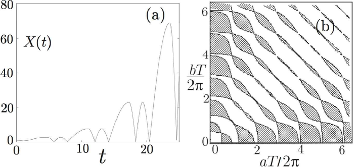
Fig. 1: Solutions of equation (27a) with $\lambda(t)$ given by (28). (a) Resonant solution for $T_{a}=10\pi,T=20\pi,a=0.05,b=0.15$ and (b) Regions of resonance for $T_{a}=T_{b}=T/2$.

As far as the regions of stability in the space of parameters are concerned, they can be obtained by studying the discriminant of equation (27a), defined as the trace of the monodromy matrix, that is

$$D(a,b,T_{a},T_{b}):=\phi_{1}(T)+\phi_{2}^{\prime}(T).$$ (29)

where $\phi_{1},\phi_{2}$ are the solutions of (27a) satisfying the initial data $\phi_{1}(0)=1,\phi_{1}^{\prime}(0)=0$ and $\phi_{2}(0)=0,\phi_{2}^{\prime}(0)=1$ respectively.

In our case it is easy to arrive at

$$\phi_{1}(T) = \cos(aT_{a})\cos(bT_{b})-\frac{a}{b}\mathop{\rm sen}\nolimits(aT_{a})\mathop{\rm sen}\nolimits(bT_{b}),$$ (30a)

$$\phi_{2}^{\prime}(T) = \cos(aT_{a})\cos(bT_{b})-\frac{b}{a}\mathop{\rm sen}\nolimits(aT_{a})\mathop{\rm sen}\nolimits(bT_{b}).$$ (30b)

Finally, the form of the discriminant is

$$D(a,b,T_{a},T_{b})=2\cos(aT_{a}+bT_{b})-\frac{(a-b)^{2}}{ab}\mathop{\rm sen}\nolimits(aT_{a})\mathop{\rm sen}\nolimits(bT_{b})$$ (31)

The Floquet theory for linear equations with periodical coefficients connects the stability of the solutions of (27a) with the value of the discriminant. The regions of resonance correspond to values of the parameters for which $|D|>2$, whereas if $|D|<2$ the solutions are bounded [44]. The equations $D(a,b,T_{a},T_{b})=2$ and $D(a,b,T_{a},T_{b})=-2$ are the manifolds that limit the regions of stability in the 4-dimensional space of parameters. In reality, defining $\alpha=aT,\beta=bT,T_{a}=\gamma T,T_{b}=(1-\gamma)T$ the number of parameters is reduced to three

$$D(\gamma,\alpha,\beta)=2\cos(\alpha\gamma+\beta(1-\gamma))-\frac{(\alpha-\beta)^{2}}{\alpha\beta}\mathop{\rm sen}\nolimits(\alpha\gamma)\mathop{\rm sen}\nolimits(\beta(1-\gamma)),$$ (32)

Therefore, the isosurfaces $D(\gamma,\alpha,\beta)=2$ and $D(\gamma,\alpha,\beta)=-2$ can be visualized in three dimensions as is shown in figure 2.

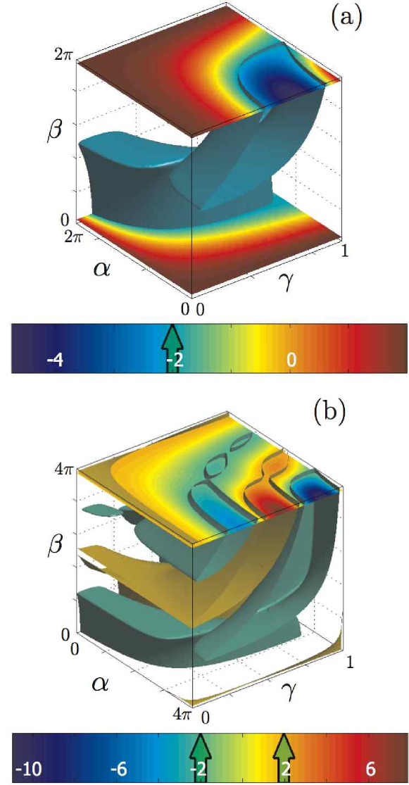
Fig. 2: (a) Isosurfaces corresponding to $D=-2$ (in this range of values $D\leq 2$) for a limited range of parameters. The regions between the gray surface and the planes limiting the drawing are regions of resonance. Sections are shown for two particular values of $\beta$ where the bluish tones correspond to the regions of resonance. The color bar indicates the color corresponding to each level of $D(\gamma,\alpha,\beta)$ and the arrow indicates the color assigned to the isosurface $D=-2$. (b) The same as (a) but for a larger range of parameters. Isosurfaces $D=2$ and $D=-2$ are shown in brown and green respectively. A section is shown for a particular value of $\beta$ with bluish and reddish tones corresponding to regions of resonances with $D<-2$ and $D>2$, respectively. In this case the two values $D=2$ and $D=-2$ are indicated by arrows on the color bar.

The general study of the regions that appear in figure 2 is complex, which leads us to focus below on a few particular cases.

For example, in the case in which the two sections have the same length $T_{a}=T_{b}$, the discriminant depends only on $aT,bT$ and it is

$$D(a,b)=2\cos\left(\frac{(a+b)T}{2}\right)-\frac{(aT-bT)^{2}}{abT^{2}}\mathop{\rm sen}\nolimits\left(\frac{aT}{2}\right)\mathop{\rm sen}\nolimits\left(\frac{bT}{2}\right)$$ (33)

so that now the condition $|D|=2$ determines curves such as those of figure 1(b).

The structure of the regions of resonance can be explored in more detail fixing the relative values of the coefficients, for example taking $b=2a$.

$$D(a,T)=2\cos\left(\frac{3aT}{2}\right)-\frac{1}{2}\mathop{\rm sen}\nolimits\left(\frac{aT}{2}\right)\mathop{\rm sen}\nolimits(aT)$$ (34)

Defining the variable $y=aT/2$, the discriminant is a function $D(y)$ [Fig. 3]. The so-called characteristic curves are hyperboles of the form $2y_{\pm}^{(n)}=aT$ being $y_{+}^{(n)},y_{-}^{(n)}$ respectively the solutions of the algebraic equations $f_{\pm}(y)=2\cos 3y-\tfrac{1}{2}\mathop{\rm sen}\nolimits y\mathop{\rm sen}\nolimits 2y\mp 2=0.$ It is easy to demonstrate that the regions of resonance are contained between two consecutive zeros of $f_{+}$ or $f_{-}$ that can be obtained using any elementary numerical method. If we draw $a$ as a function of $1/T$, the regions of resonance are those marked in colors in figure 3(b). Obviously the image is repeated due to the periodicity 2$\pi$ of $D(y)$ and there are only four basic regions of resonance (together with its harmonics) contained in the intervals (roots of $f_{+}$ and $f_{-}$): $y\in[0.84,1.23]\cup[1.91,2.3]\cup[3.98,4.37]\cup[5.05,5.44]$ (see figure 3(a)).

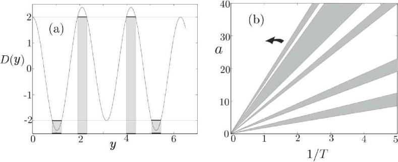
Fig. 3: (a) First four regions of resonance in $y$ (in color) for $T_{a}=T/2,b=2a$, as a function of $y=aT/2$. (b) First five regions of resonance in the plane $a-1/T$.

Another case of possible interest is that in which one of the fibers is not of GRIN type, that is, $b=0$. Then the discriminant is given by the limit of equation (31) when $b\rightarrow 0$.

$$D(a,T)=-aT\mathop{\rm sen}\nolimits{\left(\frac{aT}{2}\right)}+2\cos{\left(\frac{aT}{2}\right)}.$$ (35)

As in the previous case the only relevant parameter is $y=aT/2$, the regions of resonance on the plane $a-T$ are hyperboles and the relevant quantities are the zeroes of $f_{+}$ and $f_{-}$, which are given by

$$f_{\pm}(x)=-y\mathop{\rm sen}\nolimits y+2\cos y\mp 2=0.$$ (36)

Now there is no exact periodicity in the positions of the zeros any more, but at least it is possible to estimate the location of those of high order. To do this we must bear in mind that for $y$ big enough the dominating term in both cases is $f_{\pm}(y)\simeq-y\mathop{\rm sen}\nolimits y$, so that the zeros will be given by $y=n\pi$. It can be seen with a perturbative argument that the convergence ratio is of the order of $\mathcal{O}(1/n)$. Writing $y_{\pm}^{(n)}=n\pi+\varepsilon^{(n)}_{\pm}$ and substituting it in equations (36) it is found that

$$\varepsilon_{\pm}^{(n)}\simeq(-1)^{n+1}\frac{1\pm 2}{n\pi}.$$ (37)

This type of analysis can be extended to any restricted set of parameters.

6.2 Dynamics of Bose-Einstein condensates

In the case of Bose-Einstein condensates, there has recently been great interest in the study of the dynamics of these systems in a parametrically oscillating potential. Recent experiments (see e. g. [46, 47]) have motivated a series of qualitative theoretical analyses (the pioneer works on this subject can be seen in [48, 49, 50] although there is a great deal of posterior literature).

In the models to which we refer, the trap is modified harmonically in time, that is

$$\lambda^{2}(t)=1+\varepsilon\cos\omega t$$ (38)

with $\varepsilon>-1$. Equation (27a) with $\lambda(t)$ given by (38) is called the Mathieu equation. For this equation it is possible, as in the case of the Meissner equation, to carry out the study of the regions of the space of parameters in which resonances occur. In the first place, for any fixed $\varepsilon$, there exist two successions $\{\omega_{n}\},\,\{\omega_{n}^{\prime}\}$ with $\omega_{n},\omega^{\prime}_{n}\stackrel{{\scriptstyle n\rightarrow\infty}}{{\longrightarrow}}0$ such that if we take $\omega\in(\omega_{n},\omega_{n}^{\prime})$, equation (27a) possesses a resonance. In the second place, for fixed $\omega$, the resonances appear when $\varepsilon$ is large enough. The boundaries of those regions are the so-called characteristic curves that cannot be obtained explicitly but whose existence can be demonstrated analytically, as in the previous section, by using the discriminant. In the case of the Mathieu equation, it can be proven that the regions of instability begin in frequencies $\omega=2,1,1/2,\ldots,2/n^{2},\ldots$ [44].

As in the previous case, the resonant behavior depends only on the parameters, and not on the initial data. With respect to stability, the Massera theorem implies that if $(\varepsilon,\omega)$ is in a region of stability, then there exists a periodic solution of (27a), and by the nonlinear superposition principle such a solution is stable in the sense of Liapunov.

7 Approximate methods (I): Quadratic phase approximation (QPA)

7.1 Introduction and justification of the QPA

Up to now, the results we have shown for the evolution of the solution moments are exact and in some sense rigorous. Unfortunatelly, in many situations of practical interest it is not possible to obtain closed evolution equations for the moments. In this section we will deal with an approximate method which is based on the method of moments.

The idea of this method is to approximate the phase of the solution $u$ by a quadratic function of the coordinates, that is

$$u(x,t)=U(x,t)\exp\left(i\sum_{j=1}^{n}\beta_{j}x_{j}^{2}\right),$$ (39)

where $U(x,t)$ is a real function.

Why use a quadratic phase? Although there is not a formal justification and we do not know of any rigorous error bounds for the method to be presented here, there are several reasons which can heuristically support the use of this ansatz for the phase for situations where there are no essential shape changes of the solutions during the evolution. First of all, when Eq. (7) has self-similar solutions, they have exactly a quadratic phase [45]. Secondly, the dynamics of the phase close to stationary solutions of the classical cubic NLS equation in two spatial dimensions (critical case) is known to be approximated by quadratic phases [14, 16] Finally, to capture the dynamics of the phase of solutions close to the stationary ones, which have a constant phase, by means of a polynomial fit, the terms of lowest order are quadratic since the linear terms in the phase may be eliminated by using Theorem 2.

We would like to remark that a frequently used approach in the physical sciences to study the evolution of solutions of Eq. (1) is the so called collective coordinate method (also called averaged lagrangian method or variational method) where an specific ansatz for the solution is proposed depending on a finite number ($S$) of free parameters $u(x,t)=\varphi(x,p_{1}(t),...p_{S}(t))$. The equations for the evolution of the parameters are then sought from variational arguments [20, 21]. For NLS equations all commonly used ansatzs have a quadratic phase. Our systematic method provides a more general framework in which other methods can be systematized and understood.

As we will see in what follows, the choice (39) allows to obtain explicit evolution equations and solves the problem of calculating the integrals of the phase derivatives in the equations (12).

7.2 Modulated power-type nonlinear terms

Under the QPA, for modulated power-type nonlinearities $g(\rho,t)=g_{0}(t)\rho^{p/2}$, $p\in\mathbb{R}$ for which $\int_{\mathbb{R}^{n}}D(\rho)dx=-pJ/2$, the moment equations (12) are

$$\frac{dI_{2,j}}{dt} = V_{1,j},$$ (40a)

$$\frac{dV_{1,j}}{dt} = 4K_{j}-2\lambda_{j}^{2}I_{2,j}+pJ,$$ (40b)

$$\frac{dK_{j}}{dt} = -\frac{1}{2}\lambda_{j}^{2}V_{1,j}+p\beta_{j}J,$$ (40c)

$$\frac{dJ}{dt} = -p\left(\sum_{j=1}^{n}\beta_{j}\right)J+\frac{1}{g_{0}}\frac{dg_{0}}{dt}J.$$ (40d)

To these equations we must add the identity $V_{1,j}=4\beta_{j}I_{2,j}$, which is directly obtained by calculating $V_{1,j}$. Or, expressed otherwise

$$\beta_{j}=\frac{\dot{I}_{2,j}}{4I_{2,j}}.$$ (41)

Let us now consider the simplest case of solutions with spherical symmetry with $\lambda_{j}=\lambda(t)$, $j=1,\ldots,n$, for which $\phi(x_{1},...,x_{n})=\beta(t)\left(x_{1}^{2}+...+x_{n}^{2}\right)$. Using the same notation as in Eqs. (16) the moment equations become

$$\frac{d\mathcal{I}}{dt} = \mathcal{V},$$ (42a)

$$\frac{d\mathcal{V}}{dt} = 4\left(\mathcal{K}+\frac{np}{4}J\right)-2\lambda^{2}\mathcal{I},$$ (42b)

$$\frac{d\mathcal{K}}{dt} = -\frac{1}{2}\lambda^{2}\mathcal{V}+np\beta J,$$ (42c)

$$\frac{dJ}{dt} = -np\beta J+\frac{1}{g_{0}}\frac{dg_{0}}{dt}J$$ (42d)

with $\mathcal{V}=4\beta\mathcal{I}.$ Despite the complexity of the system of equations (42) it is possible to find two positive invariants

$$\mathcal{Q}_{1} = 2\mathcal{K}\mathcal{I}-\mathcal{V}^{2}/4,$$ (43a)

$$\mathcal{Q}_{2} = \frac{np}{2g_{0}}\mathcal{I}^{np/4}J.$$ (43b)

The existence of these invariants provides $J$ as a function of $\mathcal{I}$, which allows us to arrive at an equation for $X=\mathcal{I}^{1/2}$

$$\frac{d^{2}X}{dt^{2}}+\lambda^{2}(t)X=\frac{\mathcal{Q}_{1}}{X^{3}}+g_{0}(t)\frac{\mathcal{Q}_{2}}{X^{np/2+1}}.$$ (44)

Again we obtain a Hill’s equation with a singular term. Note that in the case $n=3,p=2$ we have a quartic term in the denominator, which corresponds with the type of powers that appear in the equations which are obtained in the framework of averaged Lagrangian methods [20].

The quadratic phase method provides reasonably precise results that at least desribe the qualitative behavior of the solutions of the partial differential equation. Using several numerical methods, we have carried out different tests especially in the most realistic case $np=6$ in (7). For example, in figure 4 the results of a simulation of (7) with $n=3$, $p=2$, $\lambda^{2}(t)=1+0.1\sin(2.8t)$ and $g_{0}=10$ are presented for an initial datum $u_{0}(x)=e^{-x^{2}/2}/\pi^{3/4}$. In this case the simplified equation (44) predicts quasi-periodic solutions which is what we obtain when resolving the complete problem.

In Fig. 5 we show the results for $\lambda^{2}(t)=1+0.1\sin(2.1t)$ for which (44) predicts resonant solutions. Again, the results of the two models are in good agreement.

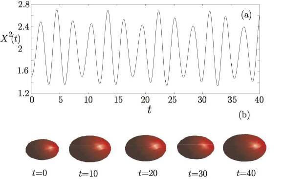
Fig. 4: Solutions of (7) in three dimensions with $p=2$, $\lambda^{2}(t)=1+0.1\sin(2.8t)$ and $g_{0}=10$ with initial data $u_{0}(x)=e^{-x^{2}/2}/\pi^{3/4}$. (a) $X^{2}(t)$ obtained numerically from the solutions on the 3D grid. (b) Isosurfaces for $|u|^{2}=0.02$ on the spatial region $[-3,3]\times[-3,3]\times[-3,3]$ and different instants of time showing the oscillations of the solution

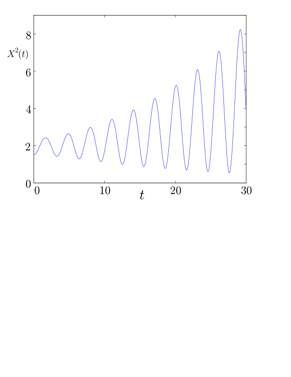
Fig. 5: Results of the simulation of (7) in three dimensions on a grid of $64\times 64\times 64$ with $\Delta t=0.005$ for $p=2$, $\lambda^{2}(t)=1+0.1\sin(2.1t)$. $X^{2}(t)$ obtained numerically from the solutions on the 3D grid is shown.

Another interesting application of the quadratic phase approximation method is the case of cubic nonlinearity, $g(\rho,t)=g_{0}(t)\rho=g_{0}(t)|u|^{2}$, without potential $\lambda(t)=0$. In that situation Eq. (44) becomes

$$\frac{d^{2}X}{dt^{2}}=\frac{\mathcal{Q}_{1}}{X^{3}}+g_{0}(t)\frac{\mathcal{Q}_{2}}{X^{n+1}}$$ (45)

where the conserved quantities are

$$\mathcal{Q}_{1} = 2\mathcal{K}\mathcal{I}-\mathcal{V}^{2}/4,$$ (46a)

$$\mathcal{Q}_{2} = \frac{n}{g_{0}}\mathcal{I}^{n/2}J.$$ (46b)

This model describes the propagation of light in nonlinear Kerr media as well as the dynamics of trapless Bose-Einstein condensates. In this situation the previous equations are used to study the possibility of stabilizing unstable solutions of the NLS equation by means of an appropriate temporal modulation of the nonlinear term, that is, by choosing a suitable function $g_{0}(t)$ thus providing an alternative to more heuristic treatments [51, 52, 53]. More details can be seen in Ref. [54].

7.3 Closure of the equations in other cases

We have just seen that the quadratic phase approximation method allows us to close the moment equations in the case of power-type nonlinear terms. Following those ideas we have managed to close the equations in more general cases.

We start from the evolution equations for the mean moments (18), that after performing the quadratic phase approximation become

$$\frac{d\mathcal{I}}{dt} = \mathcal{V},$$ (47a)

$$\frac{d\mathcal{V}}{dt} = 4\mathcal{K}-2\lambda^{2}\mathcal{I}-2n\int_{\mathbb{R}^{n}}D(\rho,t),$$ (47b)

$$\frac{d\mathcal{K}}{dt} = -\frac{1}{2}\lambda^{2}\mathcal{V}-2n\beta\int_{\mathbb{R}^{n}}D(\rho,t),$$ (47c)

$$\frac{dJ}{dt} = 2n\beta\int_{\mathbb{R}^{n}}D(\rho,t)+\int_{\mathbb{R}^{n}}\frac{\partial G(\rho,t)}{\partial t}.$$ (47d)

and $\mathcal{V}=4\beta\mathcal{I}$.

The idea to close the previous equations is to calculate the evolution of $\int_{\mathbb{R}^{n}}D(\rho,t)dx$, which is the term that prevent us from closing the equations, and try to write this evolution in terms of the moments. Let us define a new moment $\mathcal{F}$ as

$$\mathcal{F}(t)=\int_{\mathbb{R}^{n}}D(\rho,t)dx=J-\int_{\mathbb{R}^{n}}\rho\frac{\partial G(\rho,t)}{\partial\rho}dx.$$ (48)

Then, the evolution equations are

$$\frac{d\mathcal{I}}{dt} = \mathcal{V},$$ (49a)

$$\frac{d\mathcal{V}}{dt} = 4\mathcal{K}-2\lambda^{2}\mathcal{I}-2n\mathcal{F},$$ (49b)

$$\frac{d\mathcal{K}}{dt} = -\frac{1}{2}\lambda^{2}\mathcal{V}-2n\beta\mathcal{F},$$ (49c)

$$\frac{dJ}{dt} = 2n\beta\mathcal{F}+\int_{\mathbb{R}^{n}}\frac{\partial G}{\partial t}dx,$$ (49d)

together with the evolution of $\mathcal{F}$

$$\frac{d\mathcal{F}}{dt}=2n\beta F+2n\beta\int_{\mathbb{R}^{n}}\rho^{2}\frac{\partial^{2}G}{\partial\rho^{2}}dx+\int_{\mathbb{R}^{n}}\frac{\partial G}{\partial t}dx-\int_{\mathbb{R}^{n}}\rho\frac{\partial}{\partial t}\frac{\partial G}{\partial\rho}dx.$$ (50)

To try to close the system of equations (49)-(50) we impose that $\int_{\mathbb{R}^{n}}\rho^{2}\frac{\partial^{2}G}{\partial\rho^{2}}dx$ is a linear combination of $\mathcal{F}$ and $J$

$$\int_{\mathbb{R}^{n}}\rho^{2}\frac{\partial^{2}G}{\partial\rho^{2}}dx=a_{\mathcal{F}}\mathcal{F}+a_{J}J=(a_{\mathcal{F}}+a_{J})\int_{\mathbb{R}^{n}}Gdx-a_{\mathcal{F}}\int_{\mathbb{R}^{n}}\rho\frac{\partial G}{\partial\rho}dx,$$ (51)

where $a_{\mathcal{F}}$ and $a_{J}$ are two arbitrary constants. Then, $G$ must verify

$$\int_{\mathbb{R}^{n}}\left[\rho^{2}\frac{\partial^{2}G}{\partial\rho^{2}}+a_{\mathcal{F}}\rho\frac{\partial G}{\partial\rho}-(a_{\mathcal{F}}+a_{J})G\right]=0.$$

Therefore, if the nonlinear term $g(\rho)$ in the NLS equation is such that $G(\rho)$ verifies Euler’s equation

$$\rho^{2}\frac{\partial^{2}G}{\partial\rho^{2}}+a_{\mathcal{F}}\rho\frac{\partial G}{\partial\rho}-(a_{\mathcal{F}}+a_{J})G=0,$$ (52)

the evolution equations will close. In that case we can write $G(\rho,t)=g_{0}(t)G_{1}(\rho)$, where $g_{0}(t)$ is an arbitrary function which indicates the temporal variation of the nonlinear term and $G_{1}(\rho)$ satisfies Eq. (52). So

$$\int_{\mathbb{R}^{n}}\frac{\partial G}{\partial t}dx = \frac{dg_{0}}{dt}\int_{\mathbb{R}^{n}}G_{1}(\rho)dx=\frac{1}{g_{0}}\frac{dg_{0}}{dt}J(t),$$

$$\int_{\mathbb{R}^{n}}\rho\frac{\partial}{\partial t}\frac{\partial G}{\partial\rho}dx = \frac{dg_{0}}{dt}\int_{\mathbb{R}^{n}}\rho\frac{dG_{1}}{d\rho}=\frac{1}{g_{0}}\frac{dg_{0}}{dt}[J(t)-\mathcal{F}(t)],$$

and the moment equations are written as

$$\frac{d\mathcal{I}}{dt} = \mathcal{V},$$ (54a)

$$\frac{d\mathcal{V}}{dt} = 4\mathcal{K}-2\lambda^{2}\mathcal{I}-2n\mathcal{F},$$ (54b)

$$\frac{d\mathcal{K}}{dt} = -\frac{1}{2}\lambda^{2}\mathcal{V}-2n\beta\mathcal{F},$$ (54c)

$$\frac{dJ}{dt} = 2n\beta\mathcal{F}+\frac{1}{g_{0}}\frac{dg_{0}}{dt}J,$$ (54d)

$$\frac{d\mathcal{F}}{dt} = 2n\beta(1+a_{\mathcal{F}})\mathcal{F}+2n\beta a_{J}J+\frac{1}{g_{0}}\frac{dg_{0}}{dt}\mathcal{F}.$$ (54e)

By solving Eq. (52) we obtain specific nonlinear terms for which the quadratic phase approximation allows us to write closed equations for the moments. Depending on the parameter $\delta=(1+a_{\mathcal{F}})^{2}+4a_{J}$ there exist three families of solutions

$$G_{1}(\rho)=\begin{cases}C_{1}\rho^{p_{+}}+C_{2}\rho^{p_{-}},\ \delta>0,\\ C_{1}\rho^{R}+C_{2}\rho^{R}\log\rho,\ \delta=0,\\ C_{1}\rho^{R}\cos(I\log\rho)+C_{2}\rho^{R}\sin(I\log\rho),\ \delta<0,\end{cases}$$ (55)

where $p_{\pm}=\left((1-a_{\mathcal{F}})\pm\delta^{1/2}\right)/2,$ $R=\left(1-a_{\mathcal{F}}\right)/2$, $I=|\delta|^{\frac{1}{2}}/2$.

The most interesting case for applications is $\delta>0$ the nonlinear term being of the form

$$g_{1}(\rho)=k_{1}\rho^{p_{+}-1}+k_{2}\rho^{p_{-}-1},$$ (56)

where $k_{1}$ and $k_{2}$ are arbitrary constants and $p_{+}$ and $p_{-}$ are defined through the relations

$$a_{\mathcal{F}} = 1-p_{+}-p_{-},$$ (57a)

$$a_{J} = -(p_{+}-1)(p_{-}-1).$$ (57b)

Eq. (56) implies that the quadratic phase approximation allows to close the moment equations for nonlinear terms which can be written as a linear combination of two arbitrary powers of $|u|$.

As in the previous subsection it is possible to find some invariant quantities, namely

$$Q_{1} = 2\mathcal{K}\mathcal{I}-\mathcal{V}^{2}/4,$$ (58a)

$$Q_{+} = C\frac{n}{f_{+}}{\frac{\mathcal{I}^{a_{+}n}}{g_{0}}}(J+f_{+}\mathcal{F}),$$ (58b)

$$Q_{-} = C\frac{n}{f_{+}}{\frac{\mathcal{I}^{a_{-}n}}{g_{0}}}(J+f_{-}\mathcal{F}),$$ (58c)

where

$$a_{\pm}=\frac{p_{\pm}-1}{2},\ f_{\pm}=\frac{1}{p_{\mp}-1},\ C=\left(1-\frac{f_{-}}{f_{+}}\right)^{-1}=\left(1-\frac{p_{-}-1}{p_{+}-1}\right)^{-1}.$$ (59)

These conserved quantities allow us to write a differential equation for the dynamical width $X(t)=\mathcal{I}^{1/2}$

$$\frac{d^{2}X}{dt^{2}}+\lambda^{2}(t)X=\frac{\mathcal{Q}_{1}}{X^{3}}+g_{0}(t)\left(\frac{\mathcal{Q}_{-}}{X^{2a_{-}n+1}}-\frac{\mathcal{Q}_{+}}{X^{2a_{+}n+1}}\right).$$ (60)

The most interesting kind of nonlinearity in the form of Eq. (56) is the so-called cubic-quintic nonlinearity for which $g_{0}(t)=1,\ g_{1}(\rho)=k_{1}\rho+k_{2}\rho^{2}=k_{1}|u|^{2}+k_{2}|u|^{4}$. Then, we have $p_{+}-1=2$, $p_{-}-1=1$, $a_{\mathcal{F}}=-4$, $a_{J}=-2$, $a_{+}=1$, $f_{+}=1$, $a_{-}=1/2$, $f_{-}=1/2$, $C=2$. The invariant quantities are

$$\mathcal{Q}_{1} = 2\mathcal{K}\mathcal{I}-\mathcal{V}^{2}/4,$$ (61a)

$$\mathcal{Q}_{+} = 2n\mathcal{I}^{n}(J+\mathcal{F}),$$ (61b)

$$\mathcal{Q}_{-} = 2n\mathcal{I}^{n/2}(J+\mathcal{F}/2),$$ (61c)

and the equation for the width is

$$\frac{d^{2}X}{dt^{2}}+\lambda^{2}(t)X=\frac{\mathcal{Q}_{1}}{X^{3}}+\frac{\mathcal{Q}_{-}}{X^{n+1}}-\frac{\mathcal{Q}_{+}}{X^{2n+1}}$$ (62)

These equations contain a finite-dimensional description of the dynamics of localized solutions of the model and are similar to those found under specific assumptions for the profile $u(x,t)$ (see e.g. [55, 56, 57]). The main difference is that the method of moments allows to obtain the equations under minimal assumptions on the phase of the solutions and that depend on general integral quantities related to the initial data $\mathcal{Q}_{1},\mathcal{Q}_{+},\mathcal{Q}_{-}$. This is an essential advantage over the averaged Lagrangian methods used in the literature for which the specific shape of the solution must be chosen a priori (see also [20, 45]).

8 Approximate methods (II): Thomas-Fermi Limit

8.1 Concept

In the framework of the application of the NLS equations to Bose-Einstein condensation problems (thus for nonlinearities of the form $g(\rho)=g_{0}\rho$), the Thomas-Fermi limit corresponds to the case $g_{0}\gg 1$ (note that this is only one of the many different meanings of “Thomas-Fermi” limit in physics).

Usually, what is pursued in this context is to characterize the ground state, defined as the stationary solution of the NLS equation given by Eq. (11) with fixed $L^{2}$ norm having minimal energy $E$. It is also interesting to find the dynamics of the solutions under small perturbations of the ground state solution.

8.2 Physical treatment

Let us consider the problem of characterizing the ground state of (7). The usual “physical” way of dealing with this problem consists of assuming that if the nonlinear term is very large then it would be possible to neglect the Laplacian term in (7) (!) and to obtain the ground state solution as

$$\varphi_{TF}(x)=\sqrt{\left(\frac{\mu-\frac{1}{2}\sum\lambda_{j}^{2}x_{j}^{2}}{g_{0}}\right)_{+}}.$$ (63)

The value of $\mu$ is obtained from the condition of normalization $\left\|\varphi_{TF}\right\|_{2}=1$. This procedure provides a solution without nodes which is then argued to be an approximation to the ground state.

This method is used in many applied works, but unfortunately it is not even self-consistent. Near the zero of the radicand of (63) the approximation obtained has divergent derivatives, which contradicts the initial hypothesis of “smallness” of the Laplacian term. Although several numerical results can be obtained using this approximation, its foundation is very weak.

In order to understand the problem better, we rewrite (7) making the change of variables $\kappa=\mu/g_{0}$, $\eta=x/\sqrt{g_{0}}$, $\psi(\eta)=\varphi\left(x/\sqrt{g_{0}}\right)$, to give us the equation

$$-\frac{1}{2}\epsilon^{2}\Delta\psi+\frac{1}{2}\left(\sum_{j}\lambda_{j}^{2}\eta_{j}^{2}\right)\psi+|\psi|^{2}\psi=-\kappa\psi,$$ (64)

with $\epsilon=1/g_{0}$. It is evident that $\epsilon^{2}\Delta\psi$ is a singular perturbation whose effect may not be trivial.

8.3 The method of moments and the Thomas-Fermi limit

What can be said for the case of power-type nonlinearities in the limit $g\gg 1$ on the basis of the method of moments? Before making any approximations we write an evolution equation for $\mathcal{I}$ as follows. For the sake of simplicity, though it is not strictly necessary, we will consider the case of $\lambda_{j}=\lambda$ for $j=1,...,n$ and study the equations for the mean values (16).

First, we write Eqs. (17a) and (17b)

$$\frac{d\mathcal{I}}{dt} = \mathcal{V},$$ (65a)

$$\frac{d\mathcal{V}}{dt} = 4\left(\mathcal{K}+\frac{np}{4}J\right)-2\lambda^{2}\mathcal{I}=(4-np)\mathcal{K}+np\mathcal{H}-\left(2+\frac{np}{2}\right)\lambda^{2}\mathcal{I}.$$ (65b)

where $\mathcal{H}$ is the conserved energy. Combining (65a) and (65b) we arrive at

$$\frac{d^{2}\mathcal{I}}{dt^{2}}+\left(2+\frac{np}{2}\right)\lambda^{2}\mathcal{I}=(4-np)\mathcal{K}+np\mathcal{H}.$$ (66)

Equation (66) is exact.

The fact that the energy functional $E$ reaches a miminum over $\varphi_{0}$ implies, by Lyapunov stability, that initial data $u_{0}(x)=\varphi_{0}(x)+\varepsilon\delta(x)$ close to the ground state must remain proximal for sufficiently small values of $\varepsilon$.

The only approximation needed to complete our analysis is to assume that when $g\gg 1$ then $J\gg\mathcal{K}$ for the ground state. Notice that this is a much more reasonable assumption than the direct elimination of the second derivative in the evolution equation. Thus, the energy conservation and the previous considerations allow us to affirm that $J(t)\gg\mathcal{K}(t)$ for all times.

Although these facts can be used to write explicit bounds for $\mathcal{K}$, as a first approximation and just in order to show the power of these ideas we can simply take $\mathcal{K}\simeq 0$. Under this approximation we have

$$\frac{d^{2}\mathcal{I}}{dt^{2}}+\left(2+\frac{np}{2}\right)\lambda^{2}\mathcal{I}\approx np\mathcal{H}.$$ (67)

whose solutions can be obtained explicitly as

$$\mathcal{I}(t)\simeq\frac{np\mathcal{H}}{\lambda^{2}\left(2+\frac{np}{2}\right)}+A\cos\left(\lambda t\sqrt{2+\frac{np}{2}}\right)+B\mathop{\rm sen}\nolimits\left(\lambda t\sqrt{2+\frac{np}{2}}\right).$$ (68)

The equilibrium point of Eq. (66) (corresponding to $A=B=0$) gives us the “size” of the ground state as a function of the physical parameters. Also the frequency of the oscillations around the equilibrium point is immediately obtained from Eq. (68)

$$\Omega=\lambda\sqrt{2+\frac{np}{2}}.$$ (69)

We have performed numerical simulations of the partial differential equations (7) to verify this prediction. Specifically, taking $g=5000,20000$, $\lambda=1$ and initial data of the form $u_{0}(x)=\varphi_{0}((1+\varepsilon)x)/\sqrt{1+\varepsilon}$ for $\varepsilon=0.01$ and $\varepsilon=0.02$, we find a numerical frequency of $\Omega_{\text{num}}=2.26$ which is in excellent agreement with the value provided by our Thomas-Fermi formula $\Omega_{\text{TF}}=\sqrt{8}=2.24$.

9 Summary and Conclusions

In this paper we have developed the method of moments for Nonlinear Schödinger equations. First we have found the general expressions of the method and classified the nonlinearities for which it allows a closed explicit solution of the evolution of the moments. We have also discussed several applications of the method such as the dynamics of Kerr beams in nonlinear stratified media and the dynamics of parametrically forced Bose-Einstein condensates.

Approximate techniques based on the method of moments are also discussed in this paper. In particular, the quadratic phase approximation is also developed here and applied to different problems, such as the writing of simple equations describing the stabilization of solitonic structures by control of the nonlinear terms and the dynamics of localized structures in cubic-quintic media. Finally, we have also studied the moment equations in the so-called Thomas-Fermi limit.

References

- [1] L. Vázquez, L. Streit, V. M. Pérez-García, Eds., Nonlinear Klein-Gordon and Schrödinger systems: Theory and Applications, World Scientific, Singapur (1997).
- [2] F. Brezzi, P. A. Markowich, The three-dimensional Wigner-Poisson problem: existence, uniqueness and approximation, Math. Mod. Meth. Appl. Sci. 14 (1991) 35.
- [3] J. L. López, J. Soler, Asymptotic behaviour to the 3D Schrödinger/Hartree-Poisson and Wigner-Poisson systems, Math. Mod. Meth. in App. Sci., 10 (2000), 923-943.
- [4] Y. Kivshar, G. P. Agrawal, Optical Solitons: From fibers to Photonic crystals, Academic Press (2003).
- [5] A. Hasegawa, Optical Solitons in Fibers, Springer-Verlag, Berlin, (1989).
- [6] R.K. Dodd, J.C. Eilbeck, J.D. Gibbon, H.C. Morris, Solitons and nonlinear wave equations, Academic Press, New York (1982).
- [7] J. L . Rosales, J. L. Sánchez-Gómez, Nonlinear Schödinger equation coming from the action of the particles gravitational field on the quantum potential, Phys. Lett. A 66 (1992) 111-115.
- [8] R. Fedele, G. Miele, L. Palumbo, V. G. Vaccaro, Thermal wave model for nonlinear longitudinal dynamics in particle accelerators, Phys. Lett. A 173 (1993) 407-413.
- [9] F. Dalfovo, S. Giorgini , L. P. Pitaevskii , S. Stringari, Theory of Bose-Einstein condensation in trapped gases, Rev. Mod. Phys. 71:463-512 (1999).
- [10] A.S. Davydov, Solitons in Molecular Systems Reidel, Dordrecht (1985).
- [11] A. Scott, Nonlinear Science: Emergence and dynamics of coherent structures, Oxford Appl. and Eng. Mathematics, Vol. 1, Oxford (1999).
- [12] V. E. Zaharov, V. S. L’vov, S. S. Starobinets, Sov. Phys. Usp., 17 896 (1975).
- [13] C. Sulem, P. Sulem, The nonlinear Schrödinger equation: Self-focusing and wave collapse, Springer, Berlin (2000).
- [14] G. Fibich, G. Papanicolau, Self-focusing in the perturbed and unperturbed nonlinear Schrödinger equation in critical dimension, SIAM J. Appl. Math. 60 (1999) 183-240.
- [15] V. M. Pérez-García, M. A. Porras, L. Vázquez, The nonlinear Schrödinger equation with dissipation and the moment method, Phys. Lett. A 202, 176-182 (1995).
- [16] G. Fibich, Self-focusing in the damped nonlinear Schrödinger equation, SIAM J. Appl. Math. 61, 1680-1705 (2001).
- [17] Zhi-Qiang Wang, Existence and Symmetry of multibump solutions for Nonlinear Schrödinger equations, Jour. Diff. Eqn. 159, 102-137 (1999).
- [18] G. Velo, Mathematical aspects of the nonlinear Schrödinger equation, pp. 39-67 in Nonlinear Klein-Gordon and Schrödinger systems: Theory and Applications, L. Vázquez, L. Streit, V. M. Pérez-García, Eds., World Scientific, Singapore (1996).
- [19] D. G. de Figueiredo, Y. H. Ding, Solutions of a nonlinear Schrödinger equation, Discr. Cont. Dyn. Sys. B, 3, 563-584 (2002).
- [20] B. Malomed, Variational methods in nonlinear fiber optics and related fields, Progress in Optics 43, 70-191.
- [21] A. Sánchez, A. R. Bishop, Collective coordinates and length-scale competition in spatially inhomogeneous soliton-bearing equations, SIAM Rev. 40, 579-615 (1999).
- [22] V. I. Talanov, Focusing of light in cubic media, JETP Lett. 11, 199 (1970).
- [23] M. A. Porras, J. Alda, E. Bernabeu, Nonlinear propagation and trasformation of arbitrary laser beams by means of the generalized ABCD formalism, Appl. Opt. 32, 5885-5892 (1993).
- [24] Y. Oh, Cauchy problem and Ehrenfest’s law of Nonlinear Schrödinger equations with potentials, Jour. Diff. Eqn. 81, 255-274 (1989).
- [25] E. H. Lieb, M. Loss, Analysis, Graduate Studies in Mathematics, Vol. 14, American Mathematical Society (1996).
- [26] N. Smith, F. M. Knox, N. J. Doran, K. J. Blow, I. Bennion, Enhanced power solitons in optical fibres with periodic dispersion management, Electron. Lett. 32, 54-55 (1996).
- [27] I. Gabitov, E. Shapiro, S. Turitsyn, Asymptotic breathing pulse in optical transmission systems with dispersion compensation, Phys. Rev. E 55, 3624 (1997).
- [28] S. Kumar, A. Hasegawa, Quasi-soliton propagation in dispersion-managed optical fibers, Opt. Lett. 22, 372-374 (1997).
- [29] S. Turitsyn, Stability of an optical soliton with Gaussian tails, Phys. Rev. E 56, R3784-R3787 (1997).
- [30] J. J. García-Ripoll, V. M. Pérez-García, P. Torres, Extended parametric resonances in Nonlinear Schrödinger systems, Phys. Rev. Lett. 83, 1715-1718 (1999).
- [31] V. M. Pérez-García, P. Torres, J. J. García-Ripoll, H. Michinel, Moment analysis of paraxial propagation in a nonlinear graded index fiber, Jour. Opt. B: Quant. and Semiclass. Opt., 2, 353-358 (2000).
- [32] V. M. Pérez-García, H. Michinel, H. Herrero, Bose-Einstein solitons in highly asymmetric traps, Phys. Rev. A, 57, 3837-3842 (1998).
- [33] J. J. García-Ripoll, V. M. Pérez-García, V. Vekslerchik, Construction of exact solutions by spatial traslations in inhomogenous nonlinear Schrödinger equations, Phys. Rev. E, 64, 056602-1:6 (2001).
- [34] M. A. Porras, Ph. D Thesis, Universidad Complutense (1994).
- [35] A. Gammal, T. Frederico, L. Tomio, F. Kh. Abdullaev, Stability analysis of the dimensional nonlinear Schrödinger equation with trap and two- and three-body interactions, Phys. Lett. A 267, 305-311 (2000).
- [36] E. B. Kolomeisky, T. J. Newman, J. P. Straley, X. Qi, Low dimensional Bose Liquids: Beyond the Gross-Pitaevskii approximation, Phys. Rev. Lett. 85, 1146-1149 (2000).
- [37] Yu. B. Gaididei, J. Schjodt-Eriksen, P. Christiansen, Collapse arresting in an inhomogeneous quintic nonlinear Schrödinger model, Phys. Rev. E 60, 4877-4890 (1999).
- [38] M. I. Weinstein, On the structure and formation of singularities in solutions to nonlinear dispersive evolution equations, Commun. Part. Diff. Eqn., 11, 545-565 (1986).
- [39] V. P. Ermakov, Transformation of differential equations, Univ. Izv. Kiev. 20, 1-19 (1880).
- [40] E. Pinney, The nonlinear differential equation , Proc. Amer. Math. Soc. 1 681 (1950).
- [41] J. L. Reid, J. R. Ray, Ermakov systems, nonlinear superposition and solutions of nonlinear equations of motion, J. Math. Phys. 21, 1583-1587 (1980).
- [42] C. Rogers, W. K. Schief, Multi-component Ermakov systems: Structure and linearization, Jour. Math. Anal. Appl. 198, 194-220 (1990).
- [43] M. Plum, R. M. Redheffer, A class of second-order differential equations, Jour. Diff. Eqn. 154, 454-469 (1999).
- [44] W. Magnus, S. Winkler, Hill’s equation, Dover Publications, New York (1966).
- [45] V. M. Pérez-García, Self-similar solutions and collective coordinate methods for Nonlinear Schrödinger Equations, Physica D 191 (2004) 211 218.
- [46] D. S. Jin, J. R. Ensher, M. R. Matthews, C. E. Wieman, E. A. Cornell , Collective Excitations of a Bose-Einstein Condensate in a Dilute Gas, Phys. Rev. Lett. 77, 420-423 (1996).
- [47] M.-O. Mewes, M. R. Andrews, N. J. van Druten, D. M. Kurn, D. S. Durfee, C. G. Townsend, W. Ketterle, Collective Excitations of a Bose-Einstein Condensate in a Magnetic Trap, Phys. Rev. Lett., 77 988-991 (1996).
- [48] S. Stringari, Collective Excitations of a Trapped Bose-Condensed Gas, Phys. Rev. Lett. 77, 2360-2363 (1996).
- [49] V. M. Pérez-García, H. Michinel, J. I. Cirac, M. Lewenstein, P. Zoller, Low energy excitations of a Bose-Einstein Condensate: A time-dependent variational analysis, Phys. Rev. Lett. 77 5320-5323 (1996).
- [50] V. M. Pérez-García, H. Michinel, J. I. Cirac, M. Lewenstein, P. Zoller, Dynamics of Bose-Einstein condensates: Variational Solutions of the Gross-Pitaevskii equations, Phys. Rev. A 56 1424-1432 (1997).
- [51] H. Saito, M. Ueda, Dynamically stabilized bright solitons in a two-dimensional Bose-Einstein condensate, Phys. Rev. Lett. 90, 040403 (2003).
- [52] F. Abdullaev, J. G. Caputo, R. A. Kraenkel, B. A. Malomed, Controlling collapse in Bose-Einstein condensates by temporal modulation of the scattering length, Phys. Rev. A 67, 013605 (2003).
- [53] I. Towers, B. Malomed, Stable (2+1)-dimensional solitons in a layered medium with sign-alternating Kerr nonlinearity, J. Opt. Soc. Am. B 19, 537 (2002).
- [54] G. D. Montesinos, V. M. Pérez-García, P. Torres, Stabilization of solitons of the multidimensional nonlinear Schr dinger equation: matter-wave breathers, Physica D 191, 193 (2004).
- [55] F. Abdullaev, A. Gammal, L. Tomio, T. Frederico, Stability of trapped Bose-Einstein condensates, Phys. Rev. A 63, 043604 (2001).
- [56] Z. Jovanoski, Gaussian beam propagation in -dimensional cubic-quintic nonlinear medium, Journal of Nonlinear Optical Physics & Materials 10, (2001) 79-111.
- [57] H. Michinel, J. Campo-Taboas, R. García-Fernández, J. R. Salgueiro, M. L. Quiroga-Teixeiro, Liquid light condensates, Phys. Rev. E 65, 066604 (2002).