Incompressible Turbulence as Nonlocal Field Theory

Abstract

It is well known that incompressible turbulence is nonlocal in real space because sound speed is infinite in incompressible fluids. The equation in Fourier space indicates that it is nonlocal in Fourier space as well. Contrast this with Burgers equation which is local in real space. Note that the sound speed in Burgers equation is zero. In our presentation we will contrast these two equations using nonlocal field theory. Energy spectrum and renormalized parameters will be discussed.

I Introduction

Generic Equations in Physics, like Diffusion Equation, Schrodinger Equation are local in real space. Take Schrodinger’s equation for example:

$$-i\hbar\frac{\partial\psi}{\partial t}=-\frac{\hbar^{2}}{2m}\nabla\psi+V(\mathbf{x})\psi,$$

where $V(\mathbf{x})$ is the potential, and $\psi(\mathbf{x},t)$ is the wavefunction. Clearly, to compute $\psi(\mathbf{x},t+dt)$ given $\psi(\mathbf{x},t)$, we need the local function, and finite number of its derivatives. In this talk we investigate whether the equations for fluid flows is local or not.

Fluid flows are described by Navier-Stokes (NS) equation, continuity equation, and the equation of state given below:

$$\frac{\partial\mathbf{u}}{\partial t}+\left(\mathbf{u}\cdot\nabla\right)\mathbf{u} = -\frac{1}{\rho}\nabla p+\nu\nabla^{2}\mathbf{u},$$ (1)

$$\frac{\partial\rho}{\partial t}+\nabla\cdot\left(\rho\mathbf{u}\right) = 0,$$ (2)

$$p = p(\rho),$$ (3)

where $\mathbf{u},p,\rho$ are the velocity, pressure, and density field respectively. $\nu$is the kinematic viscosity of the fluid. We nondimensionalize the above equations by scaling the quantities appropriately, e. g., divide $\mathbf{u}$ by velocity scale $U$. Navier-Stokes equation gets modified to

$$\frac{\partial\mathbf{u}}{\partial t}+\left(\mathbf{u}\cdot\nabla\right)\mathbf{u} = -\frac{C_{s}^{2}}{U^{2}}\nabla\rho+\frac{\nu}{UL}\nabla^{2}\mathbf{u}$$ (4)

where $L$ is the length scale, and $C_{s}=\sqrt{{\frac{dp_{0}}{d\rho_{0}}}}$ is the Sound Speed. If the sound speed $C_{s}$ and $\frac{\nu}{UL}$ are finite, then we can find $\mathbf{u}(\mathbf{x},t+dt)$ and $\rho(\mathbf{x},t+dt)$ given $\mathbf{u}(\mathbf{x})$ and $\rho(\mathbf{x},t)$ ( assuming that $\mathbf{u}(\mathbf{x},t)$,$\rho(\mathbf{x},t)$, and their first and second derivatives are finite). For typical flows $\frac{\nu}{UL}$ is finite, so for finite $C_{s}$, Navier-Stokes equation is local in real space.

Note that the disturbances propagate with the sound speed. The larger the sound speed, larger the range of influence per unit time. Still the influence moves locally as long as the sound speed is finite. When the sound speed is infinite, then disturbances can propagate instantaneously, and all parts of the system starts interacting; hence the system becomes nonlocal. Hence, the equations for fluid flows become nonlocal when the sound speed is infinite, which is the case for incompressible fluids $(\delta\rho=0)$. The speed of propagation is infinite in Newton’s law of gravitation as well as in Coulomb’s interactions between the charged particles. These are some other examples of nonlocal interactions in physics.

We can abstract the above physics using a 2D mesh of spring-mass system. For finite spring constant, the disturbance propagates with a finite speed, and the physics is local. When the spring constant is very large, the physics is still local, but the range of propagation per unit time becomes quite large. Here mass is pulled-pushed by local spring only (4 of them). When the spring constant become infinite, then whole system behaves like a solid and the speed of propagation becomes infinite. This system has nonlocal interactions; the movement of the mass at a point is affected by masses and springs at large distances. In fact, in this nonlocal system, we can think of a mass connected by all other masses, like in Coulomb’s interactions or in Calegaro-Sutherland model.

Any real fluid has finite sound speed however large it may be. In practice, the fluid is considered incompressible if $C_{s}/U\gg 1$. The properties of this fluid is expected to match with the ideal incompressible fluid. This is based on an assumption that the properties of fluid with $C_{s}\rightarrow\infty$ matches with $C_{s}=\infty$, or $(C_{s}\rightarrow\infty)=(C_{s}=\infty)$. This assumption seems reasonable, but we are not aware of any strict mathematical result showing this. Note that $(\nu\rightarrow 0)\neq(\nu=0)$.

In the next section we discuss incompressible Navier-Stokes equation.

II Incompressible Navier-Stokes

Before we proceed further, we remark that for incompressible fluids the normalized $-\nabla p=-\frac{C_{s}^{2}}{U^{2}}\nabla\rho$ is finite even though $C_{s}$ is infinite. Also note that the normalized term $\frac{\nu}{UL}\nabla^{2}\mathbf{u}$ is finite.

The continuity equation yields a constraint equation

$$\nabla\cdot\mathbf{u}=0,$$

the substitution of which in NS equation gives Poission’s equation for $p$,

$$\nabla^{2}p=-\nabla\cdot\left\{\mathbf{u}\cdot\nabla\mathbf{u}\right\}$$

Therefore,

$$p(\mathbf{x},t)=\int\frac{-\nabla\cdot\left\{\mathbf{u}\cdot\nabla\mathbf{u}\right\}}{\left|\mathbf{x}-\mathbf{x}^{\prime}\right|},$$

which is the Coulomb’s operator (nonlocal). Clearly the computation of $p(\mathbf{x},t)$ and consequently that of $\mathbf{u}(\mathbf{x},t+dt)$ requires knowledge of $\mathbf{u}(\mathbf{x}^{\prime})$ at all positions. This is another way to infer that incompressible NS is nonlocal in real space. Landau Landau and Lifsitz (1987), Frisch Frisch (1995), and others reached the above conclusion.

It is customary to study NS in Fourier space. Let us investigate whether NS is local or nonlocal in Fourier space. NS equation in Fourier space is

$$\frac{\partial u_{i}(\mathbf{k},t)}{\partial t}=-ik_{j}\int u_{j}(\mathbf{q})u_{i}(\mathbf{p})+ik_{i}\frac{k_{j}k_{m}}{k^{2}}\int u_{j}(\mathbf{q})u_{m}(\mathbf{p})$$

with $\mathbf{k=p+q}$. Note that the second term arises due to pressure.

Since $u_{i}(\mathbf{k},t)$ requires knowledge of $u_{j}(\mathbf{q})u_{i}(\mathbf{p})$ where $\mathbf{p}$ and $\mathbf{q}$ could be very different from $\mathbf{k}$, hence NS is nonlocal interactions in Fourier Space. If we interpret NS in terms of energy transfer, we find that the energy is exchanged between the all the three modes of the triad. Kraichnan Kraichnan (1959) and Dar et al. Dar et al. (2001) devised formulas to measure the strength of interactions in fluid turbulence. In this paper we will use Dar et al.’s mode-to-mode formalism Dar et al. (2001) in which the energy transfer rate from Fourier mode $\mathbf{p}$ to Fourier mode $\mathbf{k}$ with Fourier mode $\mathbf{q}$ acting as a mediator is given by

$$S(\mathbf{k|p|q)}=Im[\mathbf{k}\cdot\mathbf{u}(\mathbf{q})\mathbf{u}(\mathbf{p})\cdot\mathbf{u}(\mathbf{k})].$$ (5)

The above quantity can be computed using numerical simulation or using analytic tools. Earlier, Domaradzki and Rogallo Domaradzki and Rogallo (1990) and Waleffe Waleffe (1992) calculated the above using EDQNM approximation. Recently Verma et al. Verma et al. (2004) calculated the above using field-theoretic technique. In this paper we will report analytical result obtained using first-order field-theoretic calculation. In this scheme, under the assumption of homogeneity and isotropy we obtain

$$\left\langle S(k^{\prime}|p|q))\right\rangle=\frac{T_{1}(k,p,q)C(p)C(q)+T_{2}(k,p,q)C(k)C(q)+T_{3}(k,p,q)C(k)C(p)}{\nu(k)k^{2}+\nu(p)p^{2}+\nu(q)q^{2}},$$ (6)

where $T_{i}$’s are functions of $k,p$ and $q$. To save space, we have skipped all the details for which the reader is referred to Verma et al. Verma et al. (2004).

We focus our attention on the inertial range where the interactions are self-similar. Therefore, it is sufficient to analyze $S(k^{\prime}|p|q)$ for triangles $(1,p/k,q/k)=(1,v,w)$. Since, $|k-p|\leq q\leq k+p$, $|1-v|\leq w\leq 1+v$, hence any interacting triad $(1,v,w)$ is represented by a point $(v,w)$ in the hatched region of Fig. 1 Leslie (1973).

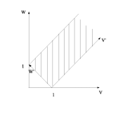
Figure 1: The interacting triad $(\mathbf{k,p,q})/k=(1,v,w)$ under the condition $\mathbf{k}=\mathbf{p+q}$ is represented by a point $(v,w)$ in the hatched region. The axis $(v^{\prime},w^{\prime})$ are inclined to axis $(v,w)$ by 45 degrees. Note that the local wavenumbers are $v\approx 1,w\approx 1$ or $v^{\prime}\approx w^{\prime}\approx 1/\sqrt{{2}}$.

For convenience, $\left\langle S(v^{\prime},w^{\prime})\right\rangle$ are represented in terms of new variables $(v^{\prime},w^{\prime})$ measured from the rotated axis shown in the figure 1. It is easy to show that $v=1+(v^{\prime}-w^{\prime})/\sqrt{{2}},w=(v^{\prime}+w^{\prime})/\sqrt{{2}}$.

The local wavenumbers are $v\approx 1,w\approx 1$, while the rest are called nonlocal wavenumbers. We substitute $C(k)$ and $\nu(k)$ in Eq. (6) and rewrite $S(k|p|q)$ in terms of $v^{\prime},w^{\prime}$. For details refer to Verma et al. Verma et al. (2004). Fig. 2 illustrates the density plots of $\left\langle S(v^{\prime},w^{\prime})\right\rangle$. Fig. (a) shows the plot for 3D, while Fig. (b) shows the one for 2D.

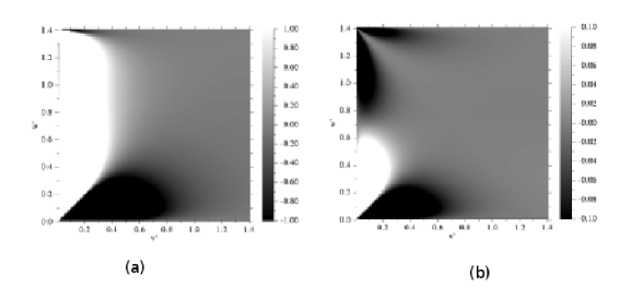
Figure 2: Density plot of $\left\langle S(v^{\prime},w^{\prime})\right\rangle$ of Eq. (6) without the bracketed factor for (a) 3D (b) 2D.

We can draw the following conclusions from the plots.

1. When $v^{\prime}\rightarrow 1$ or $v\rightarrow 0$, we find that $S(k|p|q)$ is large positive for 3D and large negative for 3D. This shows that the nonlocal interactions are strong.

2. The value of $S$ at $(v,w)=(1,1)$, or $(v^{\prime},w^{\prime})=(1/\sqrt{{2}},1/\sqrt{{2}})$ is zero in both 2D and 3D. When $v\approx w\approx 1$, $S$ is small indicating that local interactions are small.

3. When $v\rightarrow 0$, $S>0$ for 3D and $S<0$ for 2D. This is reminiscent of forward cascade in 3D, and backward cascade in 2D.

Hence, we find that the interactions in the incompressible fluid turbulence is nonlocal. This result appears to contradict Kolmogorov’s phenomenology which predicts local energy transfer in Fourier space. We will show below that the shell-to-shell energy transfer rates are local even though the interactions are nonlocal.

III Shell-to-shell energy transfers in turbulence.

The wavenumber space is divided into shells $(k_{0}s^{n},k_{0}s^{n+1})$, where $s>1$, and $n$ can take both positive and negative values. The energy transfer rate from $m$th shell $(k_{0}s^{m},k_{0}s^{m+1})$ to $n$th shell $(k_{0}s^{n},k_{0}s^{n+1})$ is given by Dar et al. (2001)

$$T_{nm}=\sum_{k_{0}s^{n}\leq k\leq k_{0}s^{n+1}}\sum_{k_{0}s^{m}\leq p\leq k_{0}s^{m+1}}\left\langle S(k|p|q)\right\rangle.$$ (7)

If the shell-to-Shell energy transfer rate is maximum for the nearest neighbours, and decreases monotonically with the increase of $|n-m|$, then the shell-to-shell energy transfer is said to be local.

$T_{nm}$ can be computed using numerical simulations or using analytical tools. Zhou Zhou (1993) calculated similar quantity. In the following we plot $T_{nm}$ obtained using numerical simulation Verma et al. (2004). Clearly, shell-to-shell energy transfer is local as envisaged by Kolmogorov.

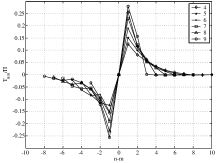
Figure 3: Plots of normalized shell-to-shell energy transfer $T_{nm}/\Pi$ vs. $n-m$ for $m=4..9$. The plots collapse on each other indicating self-similarity.

We Verma et al. (2004) have also computed the shell-to-shell energy transfer rates using field-theoretic method. The reader is referred to the original paper for the details. The plots of $T_{nm}$ for both 3D and 2D fluid turbulence given below.

Figure 4: Plot of normalized shell-to-shell energy transfer $T_{nm}/\Pi$ vs $n-m$ for $d=3$. The $n$th shell is $(k_{0}s^{n},k_{0}s^{n+1})$ with $s=2^{1/4}$. The energy transfer is maximum for $n=m\pm 1$, hence the energy transfer is local. The energy transfer is also forward.

From the above plot we can clearly deduce that energy transfer in 3D fluid turbulence is local. In fact, the values obtained from analytical calculations match very well with the numerical values shown in Fig. 3.

We have done similar analysis for 2D fluid turbulence. The result is shown below:

Figure 5: Plot of normalized shell-to-shell energy transfer $T_{nm}/\left|\Pi\right|$ vs $n-m$ for $d=2$ in the inertial range. The energy transfer rate from the shell $m$ to the shells $m+1,$ $m+2$, $m+3$ is forward, but $m+4$ onward it is negative. The net effect of all these transfer is the inverse energy flux $\Pi$.

The shell-to-shell energy transfer rates to the nearby shells are forward, whereas the transfer rates to the far off shells are backward. The net effect is a negative energy flux. This theoretical result is consistent with Dar et al.’s numerical finding Dar et al. (2001). The inverse cascade of energy is consistent with the backward nonlocal energy transfer in mode-to-mode picture [$S(k|p|q)$] (see Fig. 2). Verma et al. Verma et al. (2004) have shown that the transition from backward energy transfer to forward transfer takes place at $d_{c}\approx 2.25$.

To summarize, the triad interactions in incompressible fluids is nonlocal both in real and Fourier space. However, the shell-to-shell energy transfer is local in Fourier space. Verma et al. Verma et al. (2004) attribute this behaviour to the fact that the nonlocal triads occupy much less Fourier space volume than the local ones.

IV Fully compressible limit: Burgers equation

Let us go back to Eq. (4) and take the limit $C_{s}=0$. This is the fully compressible limit, and the resulting equation was first studied by Burgers. This equation, given below, is known as Burgers equation (strictly speaking in 1D).

$$\frac{\partial\mathbf{u}}{\partial t}+\left(\mathbf{u}\cdot\nabla\right)\mathbf{u} = \nu\nabla^{2}\mathbf{u}.$$

Clearly this equation is local in real space. What about in Fourier space?

In Fourier space, the above equation is given by

$$\frac{\partial u_{i}(\mathbf{k},t)}{\partial t}=-i\int u_{j}(\mathbf{q})p_{j}u_{i}(\mathbf{k-q})-\nu k^{2}u_{i}(\mathbf{k}),$$

which implies that the interactions are nonlocal in Fourier space. Note that the pressure term is absent in the above equation.

The field-theoretic treatment of the above equation is rather complex for arbitrary dimension. Here we attempt the self-consistent field-theoretic treatment of one-dimensional Burgers equation for 1D Burgers equation. In 1D, the energy spectrum of Burgers equation is given by

$$C(k)=A\frac{\mu^{2}}{L}k^{-2},$$ (8)

where $L$ is the length of the system, $\mu$ is the shock strength, and $A$ is a constant. Using dimensional arguments, we write the renormalized viscosity of the following form McComb (1990); Verma (2001):

$$\nu(k_{n}k^{\prime}) = \nu_{*}(k^{\prime})\mu\sqrt{{\frac{A}{L}}}k_{n}^{-3/2}.$$ (9)

Unfortunately straight-forward application of self-consistent Renormalization Group (RG) procedure of McComb McComb (1990); Verma (2001) does not work. The contributions of $<u^{>}(p)u^{>}(q)>$ is negligible; one needs to come up with a cleverer renormalization scheme to obtain the renormalized viscosity.

To make a connection with Kolmogorov’s theory of fluid turbulence, we rewrite Eq. (8) as

$$C(k)=A[\Pi(k)]^{2/3}k^{-5/3}$$

with the flux function $\Pi(k)$ as

$$\Pi(k)=\frac{\mu^{3}}{L^{3/2}}k^{-1/2}.$$ (10)

Note that the flux $\Pi$ has become $k$-dependent. Verma Verma (2000) and Frisch Frisch (1995) have shown that the flux function follows a multifractal distribution.

Question is whether we can compute the flux using field-theoretic method. Since Burgers equation is compressible, the formula $S(K|p|q)$ is not applicable Verma (2004). However we can still write the flux using Kraichnan’s combined energy transfer formula Kraichnan (1959). The energy flux crossing a wavenumber $k_{0}$ is given by

$$\Pi(k_{0}) = \int_{k>k_{0}}dk\int_{p<k_{0}}\frac{1}{2}\Im\left[-ku(p)u(q)u(k)\right],$$

with $k+p+q=0$. We apply first-order perturbative method assuming $u(k)$ to be quasi-normal as in fluid turbulence. We also make a change of variable to

$$k=\frac{k_{0}}{u};\,\,\,p=\frac{k_{0}v}{u};\,\,\,q=\frac{k_{0}w}{u}.$$

To first order,

$$\Pi(k_{0}) = \frac{k_{0}^{2}}{2}\int_{-1}^{1}du\int_{-u}^{u}(k)\frac{kC(p)C(q)+pC(k)C(q)+qC(k)C(p)}{\nu(p)p^{2}+\nu(q)q^{2}+\nu(k)k^{2}}$$

$$= \frac{A^{3/2}}{\nu_{*}}\Pi(k_{0})\int_{-1}^{1}dv\,2(1-v^{1/2})\frac{w^{-2}+v^{-2}-(vw)^{-2}}{1+v^{1/2}+w^{1/2}},$$

with $w=1-v$. We find that the above integral converges and is equal to 2.45. Hence,

$$1=\frac{A^{3/2}}{\nu_{*}}2.45.$$

Thus we show that $C(k),\nu(k),\Pi(k)$ given by Eqs. (8, 9, 10) are consistent solution of 1D Burgers equation. Note however that the renormalization group analysis of Burgers equation is somewhat uncertain.

The spectral index of Burgers equation ($-2$) is very different from the the spectral index of incompressible fluid turbulence ($-5/3$). The difference arises due to the neglect of $-\nabla p$ term in Burgers equation. The compressible effects are different in these two equations. Burgers equation is local real space, while incompressible NS is nonlocal in real space.

It is interesting to compare the above results with Noncommutative field theory, where the nonlocal interactions are included using parameter $\theta$. Burgers equation is local, while incompressible NS is nonlocal due to $-\nabla p$ term. Note that the $\nabla p$ term is nonlocal in Coulomb’s operator sense $(V\sim 1/r)$. We are not aware of field-theoretic ideas applied to Coulomb;s operator, which is one of the most important operator in physics. We hope this investigation and its connection with fluid turbulence will be carried out in future.