Links between dissipation, intermittency, and helicity in the GOY model revisited

Abstract

High-resolution simulations within the GOY shell model are used to study various scaling relations for turbulence. A power-law relation between the second-order intermittency correction and the crossover from the inertial to the dissipation range is confirmed. Evidence is found for the intermediate viscous dissipation range proposed by Frisch and Vergassola. It is emphasized that insufficient dissipation-range resolution systematically drives the energy spectrum towards statistical-mechanical equipartition. In fully resolved simulations the inertial-range scaling exponents depend on both model parameters; in particular, there is no evidence that the conservation of a helicity-like quantity leads to universal exponents.

1 Introduction

One of the most challenging aspects of turbulent fluid flow is the rapid rise in the number of active degrees of freedom as the Reynolds number increases. Given present day computational resources, this renders direct numerical simulation of the asymptotic high-Reynolds-number regime of fully developed turbulence intractable. Various reduced models of the dynamics have therefore been developed to capture the essential features of the turbulent cascade of energy from large to small scales [22, 47, 48, 49, 40, 46, 16, 17, 10, 4]. These models reflect many of the statistical features expected to influence the energy transfer in realistic flows [46, 23, 24, 25]. They have been used to study intermittency, multifractal behavior, and the scaling of energy and dissipation (see also [7, 8]). They have also been extended to include passive scalars [30], magnetic fields [6], and even polymers [2].

In this note we focus on the GOY shell model, so named after its initial proponents Gledzer [22] and Ohkitani and Yamada [47, 48, 49] (see also [10, 4] for reviews). We consider within high-resolution, fully resolved, and converged numerical simulations four related issues: the Reynolds number dependence of the crossover to the dissipation scale; the existence of an intermediate dissipation range; the effect of modal truncation in the viscous range on inertial-range scaling; and the relation between inertial-range scaling and the presence of a second conserved helicity-like quantity. Some of these aspects have been discussed for shell models in isolation before (e.g. [35, 19, 36, 37]). Key observations of the present paper are: the crossover from inertial to dissipative scales takes place at a length much smaller than the Kolmogorov estimate; these scales must be properly resolved to avoid contaminating the inertial range; and, finally, the high-resolution, fully converged simulations presented here do not support the conjecture [31] that inertial-range exponents in the helicity-preserving GOY model are universal.

The usual estimate for the scale on which dissipation begins to dominate, based on the energy dissipation density $\epsilon$ and the kinematic viscosity $\nu$, is the Kolmogorov scale

$$\eta=\left(\frac{\nu^{3}}{\epsilon}\right)^{1/4}.$$ (1)

However, numerical simulations of passive scalars show that in order to recover small-scale fluctuations, gradients, and dissipation accurately, one has to go well below this scale [43]. A straightforward line of reasoning expanded on in Sect. 3 shows that in the presence of intermittency corrections, as reflected in the energy density scaling like $k^{-5/3-\delta}$ with $0<\delta<4/3$, the dissipative range sets in at a scale $\eta_{d}$ that is a fraction of $\eta$ that decreases as the Reynolds number increases (i.e. as the viscosity decreases):

$$\eta_{d}=\eta\left(\frac{\eta}{L}\right)^{3\delta/(4-3\delta)}\sim\nu^{1/(\frac{4}{3}-\delta)}.$$ (2)

The integral or outer scale $L$ appearing here is the characteristic scale of the external stirring force. A more detailed argument for the variation of the energy density in the transition between the inertial and viscous ranges, based on the multifractal model of intermittency, shows that an intermediate dissipation range develops that widens with increasing Reynolds number [21]. In Sect. 4, we present high-resolution numerical evidence for the existence of an intermediate dissipation range in the GOY model. However, this part of the spectrum is so steep that it contributes negligibly to the energy balances used in Sect. 3 to determine the dissipation wavenumber.

As part of these studies we also considered the influence of modal truncations on spectra. If the modes are truncated very far in the viscous range, it is reasonable to expect that the behavior will not change. However, as the cutoff moves closer and closer to the dissipation scale, it begins to inhibit sufficient dissipation. As a consequence, the pileup of energy close to the transition between the inertial- and viscous-dominated regimes (the bottleneck effect, which also occurs in simulations of the Navier–Stokes equation [19, 36, 37]) is enhanced to the point where the system tends towards a weakly damped equilibrium: the distribution of energy approaches a $1/k$ scaling, corresponding to an equipartition of the energy contents of the geometrically spaced shells. A similar kind of effect has been noted in models with hyperviscosity, where the rapid quenching of high-wave number modes also effects the inertial-range scaling [35].

In Sect. 5, using fully resolved simulations, we revisit the studies of Kadanoff et al. [31, 42]. These authors considered different parameters for the GOY model and reported that the intermittency corrections fall into two categories, depending on whether or not the model preserves a helicity-like quadratic quantity. On revisiting these studies with higher-resolution simulations, we do not find such a correspondence, but rather a persistent dependence of the intermittency corrections on all parameters of the model.

Before addressing these issues, it is helpful to describe in the next section the underlying model and some related technical details.

2 Preliminaries

The GOY model has, as primary dynamical variables, complex velocities $u_{n}$ representing the velocity field in shell number $n$, where $n=0,1,\ldots,N-1$. They evolve according to

$$\left(\frac{d}{dt}+\nu k_{n}^{2}\right)u_{n}={\mathcal{S}}_{n}+F_{n},$$ (3)

where

$${\mathcal{S}}_{n}=ik_{n}\left(\alpha u_{n+1}^{*}u_{n+2}^{*}+\frac{\beta}{\lambda}u_{n-1}^{*}u_{n+1}^{*}+\frac{\gamma}{\lambda^{2}}u_{n-1}^{*}u_{n-2}^{*}\right),$$ (4)

given the boundary conditions $u_{-2}=u_{-1}=u_{N}=u_{N+1}=0$. The wavenumbers $k_{n}=k_{0}\lambda^{n}$ scale geometrically. It is customary to rescale time so that $\alpha=1$ and require that $\alpha+\beta+\gamma=0$, so that the nonlinear terms in $S_{n}$ conserve the energy $\frac{1}{2}\sum_{n}|u_{n}|^{2}$. A second invariant $\frac{1}{2}\sum_{n}k_{n}^{p}|u_{n}|^{2}$ is also conserved, where $p=-\log_{\lambda}(-\beta-1)$. Of particular interest is the case where $\lambda=1/(1+\beta)$, when this invariant takes the form of a quantity $H=\frac{1}{2}\sum_{n}(-1)^{n}k_{n}|u_{n}|^{2}$ with the same dimensions and sign indefiniteness as the helicity invariant of three-dimensional Navier Stokes turbulence.

For the standard case considered by Kadanoff et al. [31, 42], $k_{0}=2^{-3}$, $\lambda=2$, $\beta=\gamma=-1/2$, $\nu=10^{-7}$, $N=22$ and the forcing is confined to shell $3$:

$$F_{n}=f\delta_{n,3}.$$ (5)

The amplitude of the external forcing is constant: $f=5(1+i)\times 10^{-3}$. In these models, one observes an inertial-range power-law scaling of the mean shell energy $\frac{1}{2}\langle|u_{n}|^{2}\rangle\sim k_{n}^{-2/3}$, corresponding to the energy spectrum $E(k_{n})=\frac{1}{2}\langle|u_{n}|^{2}\rangle/(k_{n+1}-k_{n})\sim k_{n}^{-5/3}$ and reminiscent of the “K41” scaling predicted by the Kolmogorov theory [32]. Here $\langle\rangle$ denotes an ensemble average. At higher shell indices one observes an exponential decrease of the shell amplitudes, corresponding to a viscous range [1].

On multiplying (3) by $u_{n}^{*}$ and summing over shells $m$ to $N-1$, one arrives at the energy balance

$$\frac{d}{dt}\sum_{n=m}^{N-1}\left|\langle u_{n}\rangle\right|^{2}=\Pi_{m}-\epsilon_{m},$$ (6)

where $\Pi_{m}=2\mathop{\rm Re}\nolimits\sum_{n=m}^{N-1}\langle{\mathcal{S}}_{n}u_{n}^{*}\rangle$ represents the transfer of energy by the nonlinear terms into shells $m$ to $N-1$ and

$$\epsilon_{m}=2\nu\sum_{n=m}^{N-1}k_{n}^{2}\langle\left|u_{n}\right|^{2}\rangle-2\mathop{\rm Re}\nolimits\sum_{n=m}^{N-1}\langle F_{n}u_{n}^{*}\rangle,$$ (7)

is the total transfer, via dissipation and forcing, out of this range of shells. A positive value for $\Pi_{m}$ represents a flow of energy to shells $m$ and higher. When $\nu=0$ and $F=0$, energy conservation implies that

$$\Pi_{m}=-2\sum_{n=0}^{m-1}\langle S_{n}u_{n}^{*}\rangle,$$ (8)

so that $\Pi_{0}=\Pi_{N}=0$. In a statistical steady state, the left-hand side of (6) vanishes and $\Pi_{m}=\epsilon_{m}$. This condition serves as an excellent numerical diagnostic for discerning when a steady state has been reached. In practice, appealing to the ergodic theorem, running time averages (say from $T/2$ to the final time $T$) are used to approximate the required ensemble averages.

As pointed out in [41], it is highly advantageous to use an exponential integrator to solve (3) exactly on the linear time scale. Exponential integrators [13, 28, 3, 15, 29] are well suited to linearly stiff systems that exhibit dynamics on a wide range of time scales. They allow for much larger time steps than either classical nonstiff methods or simple integrator factor (Rosenbrock) methods [26]. However, instead of using the second-order exponential Adams–Bashforth scheme used by Pisarenko et al. [41] or the fixed time step schemes of Cox and Matthews [15], we used the exponential version [11] of the adaptive third-order Bogacki–Shampine [9] Runge–Kutta integrator described in Appendix A. With a nonstochastic forcing, this scheme can reuse the final source evaluation from the previous time step.

Instead of a constant forcing, it is also possible to apply a central white-noise stochastic forcing, where $f$ is delta-correlated in time. The advantage of this forcing is that it yields a prescribed mean energy injection $\epsilon=\frac{1}{2}\langle\left|f\right|^{2}\rangle$, independent of the lattice size and forcing [39].

The fully resolved spectra and cumulative energy transfers $\Pi_{n}$ and $\epsilon_{n}$ corresponding to a series of decreasing values of $\nu$ are shown in Fig. 1. Here we set $k_{0}=1$ and used the standard values $(\beta,\lambda)=(-1/2,2)$ with a complex-valued white-noise random forcing restricted to the first shell, such that the total energy injection $\epsilon$ is $1$. Initially all shells were assigned the same nonzero real amplitude (a statistical mechanical equipartition of energy); the complex forcing and nonlinearity then cause them to develop imaginary parts. The dashed vertical lines in Fig. 1 separate regions of equal energy dissipation, providing a convenient definition for the dissipation wavenumber $k_{d}$; namely, $2\nu\int_{0}^{k_{d}}k^{2}E(k)\,dk=\epsilon/2$. As seen by the near coincidence of $k_{d}$ with the maxima of the energy dissipation, this definition of $k_{d}$ closely approximates a point of inflection, with respect to shell number, of the cumulative energy transfer [34].

The highest resolution case was run $1.2\times 10^{9}$ adaptive time steps for a total of $9756$ time units, or roughly $4000$ large-eddy turnover times. In Fig. 2, we illustrate the power-law behavior of $k_{d}$ vs. $\nu$ evident in Fig. 1; using a least-squares fit, we find that

$$k_{d}\sim\nu^{-0.7855},$$ (9)

with the exponent determined to within a statistical error of $0.0005$. Thus, instead of the K41 value $-0.75$ arising from (1), we obtain an exponent much closer to the anomalous value $-0.775$ deduced from (2), using the second-order intermittency correction $\delta=0.0438$ measured in section 3.

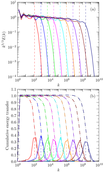
Figure 1: (a) Compensated energy densities for the GOY model driven by a white-noise random forcing, normalized by the $K41$ law, for $\nu=10^{-3}$, $10^{-4}$, $10^{-5}$, $10^{-6}$, $10^{-7}$, $10^{-8}$, $10^{-9}$, $10^{-10}$, and $10^{-11}$. (b) Cumulative energy transfer functions: the dashed (dotted) curves indicate the value of $\Pi_{n}$ ($\epsilon_{n}$) at the wavenumbers $k_{n}$. The energy dissipation $\nu k^{2}\langle\left|u_{n}\right|^{2}\rangle$ (solid curves) is maximal very near $k_{d}$ (vertical dashed lines).

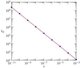
Figure 2: Scaling of $k_{d}$ vs. $\nu$ for the simulations in Fig. 1. The line joining the data points is a least-squares fit.

The slow decrease with wavenumber of the energy spectra compensated by the simple algebraic scaling indicates an intermittency correction to the exponent. The relationship between this intermittency correction and the dissipation wavenumber $k_{d}$ will be considered in the next section.

3 Intermittency-length scale paradox

Deviations of the $p$-th order structure function scaling exponents from the Kolmogorov value $p/3$ require the presence of a length scale $\ell$ for dimensional correctness:

$$S_{p}(k_{n})=\left<\left|u_{n}\right|^{p}\right>\sim\left(\frac{\epsilon}{k_{n}}\right)^{p/3}(k_{n}\ell)^{-\delta_{p}}\sim\epsilon^{p/3}k_{n}^{-\zeta_{p}}\ell^{-\delta_{p}},$$ (10)

where $\zeta_{p}=p/3+\delta_{p}$. Two natural choices for this length scale are the external, stirring scale $L$ and the small scale $\eta_{d}$ at which dissipation terminates the inertial range. Concerning this choice, we now give two elementary arguments that at first glance lead to seemingly conflicting results.

The energy spectrum may be expressed in terms of the intermittency exponent $\delta=\delta_{2}$:

$$E(k)=C\epsilon^{2/3}k^{-5/3}(k\ell)^{-\delta}.$$ (11)

On balancing the energy injection $\epsilon$ and energy dissipation between the largest scale $L$ and some dissipation scale $\eta_{d}$, one finds

$$\epsilon = 2\nu\int_{2\pi/L}^{2\pi/\eta_{d}}k^{2}E(k)\,dk=2C\nu\epsilon^{2/3}\ell^{-\delta}\int_{2\pi/L}^{2\pi/\eta_{d}}k^{1/3-\delta}\,dk$$ (12)

$$\sim \nu\epsilon^{2/3}\ell^{-\delta}\left(\frac{1}{\eta_{d}}\right)^{4/3-\delta}\qquad(\eta_{d}\ll L),$$

where we have tacitly assumed that $\delta<4/3$, so that the upper integration limit dominates. If one takes $\eta_{d}$ to be the Kolmogorov scale $\eta=(\nu^{3}/\epsilon)^{1/4}$, then on comparing the left- and right-hand sides of (12), one obtains

$$\epsilon\sim\nu\epsilon^{2/3}\left(\frac{\eta}{\ell}\right)^{\delta}\frac{\epsilon^{1/3}}{\nu}.$$ (13)

For $\delta\neq 0$, such a balance is possible only if $\ell\sim\eta$; that is, the relevant choice for $\ell$ is the dissipation scale.

On the other hand, the Cauchy–Schwarz inequality implies that structure functions satisfy [20]

$$S_{\frac{p}{2}+\frac{q}{2}}\leq S_{p}^{1/2}S_{q}^{1/2}.$$ (14)

On expressing $S_{p}\sim(\epsilon r)^{p/3}(r/\ell)^{\delta_{p}}$, where $r=2\pi/k$, one obtains a convexity condition on $\delta_{p}$:

$$\left(\frac{r}{\ell}\right)^{\delta_{\frac{p+q}{2}}}\leq\left(\frac{r}{\ell}\right)^{\frac{\delta_{p}}{2}+\frac{\delta_{q}}{2}},$$ (15)

or

$$1\leq\left(\frac{r}{\ell}\right)^{\frac{\delta_{p}+\delta_{q}}{2}-\delta_{\frac{p+q}{2}}}.$$ (16)

So if $\ell$ is the smallest excited length scale ($\ell\sim\eta$), then $r/\ell>1$ for all $r$, which would imply that $\delta_{p}$ (and hence $\zeta_{p}$) is convex. Alternatively, if $\ell$ is the largest excited length scale ($\ell\sim L$), then $r/\ell<1$ for all $r$, and $\delta_{p}$ (and hence $\zeta_{p}$) is concave.

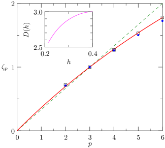
Figure 3: Concavity of structure functions exponents $\zeta_{p}$ vs. $p$ for $\beta=-0.5$ and $\lambda=2$. The circles represent numerical values obtained by a least-squares fit of the flux (21) between $k=10^{2}$ and $10^{6}$ for the case $\nu=10^{-11}$. The dashed line is the Kolmogorov prediction $\zeta_{p}=p/3$; the solid line indicates the She–Lévêque scaling $\zeta_{p}=p/9+2-2(2/3)^{p/3}$, and the squares represent the experimental values measured for 3D turbulence by van de Water & Herweijer [27]. In the inset we graph the dimension $D(h)$ determined from our numerical $\zeta_{p}$ values by inversion of the multifractal Legendre transformation.

$p$	$2$	$3$	$4$	$5$	$6$
$\zeta_{p}$	$\phantom{\pm}0.7105$	$\phantom{\pm}0.9999$	$\phantom{\pm}1.262$	$\phantom{\pm}1.503$	$\phantom{\pm}1.726$
$\Delta_{\zeta_{p}}$	$\pm 0.0005$	$\pm 0.0005$	$\pm 0.001$	$\pm 0.001$	$\pm 0.002$

Table 1: Numerically computed structure function exponents $\zeta_{p}$ and the statistical errors $\Delta_{\zeta_{p}}$ (from a least-squares fit between $k=10^{2}$ and $10^{6}$) for $\beta=-0.5$ and $\lambda=2$.

Both Navier–Stokes turbulence and the GOY model have concave exponents, as illustrated in Fig. 3 and tabulated in Table 1 for $(\beta=-1/2,\lambda=2)$. In fact, the curvature of $\zeta_{p}$ is very close to that observed experimentally for three-dimensional Navier–Stokes turbulence [27]. This supports $\ell=L$ (see also Ref. [18]), even though (13) appears to require that $\ell=\eta$. The above calculations assume spectra with a sharp cut-off at the dissipation scale, but the same analysis with the same conclusion can be performed for spectra with an exponential cut-off.

This apparent contradiction is easily resolved: a steeper-than-Kolmogorov spectrum necessitates integrating to scales smaller than $\eta$ to obtain sufficient dissipation [21]. If we set $\eta_{d}\sim\eta\left(\frac{\eta}{L}\right)^{\sigma}$, we obtain the energy balance

$$1\sim\left(\frac{\eta}{\ell}\right)^{\delta}\left(\frac{\eta}{L}\right)^{\sigma(\delta-4/3)}.$$ (17)

This is consistent with $\ell=L$ if $\delta+\sigma(\delta-4/3)=0$, that is, if

$$\sigma^{-1}=\frac{4}{3}\delta^{-1}-1.$$ (18)

For $0<\delta<4/3$, we see that $\sigma>0$. The conclusion is that the inertial range extends to a scale $\eta_{d}$ that is smaller than the Kolmogorov scale $\eta$:

$$\eta_{d}\sim\eta\left(\frac{\eta}{L}\right)^{\sigma}\sim\eta^{1+\sigma}=\left(\frac{\nu^{3}}{\epsilon}\right)^{\frac{(1+\sigma)}{4}},$$ (19)

for a fixed outer scale $L$. When the energy injection $\epsilon$ is also fixed, we thus have

$$\eta_{d}\sim\nu^{1/(\frac{4}{3}-\delta)}.$$ (20)

Equivalently, on setting $\ell=L$, one can obtain that this scaling directly from (12).

To verify this relation numerically, we followed Kadanoff et al. [42] and computed $\zeta_{p}$ via a least-squares fit of the time-averaged $p$th-order flux

$$\Sigma_{n,p}=\left<\left|\mathop{\rm Im}\nolimits\left(u_{n}u_{n+1}u_{n+2}+\frac{1+\beta}{\lambda}u_{n-1}u_{n}u_{n+1}\right)\right|^{p/3}\right>,$$ (21)

in order to filter out the well-known period-three oscillation in solutions of the GOY model [41]. We chose the interval $[10^{2},10^{6}]$ for doing the least-squares fit, as the logarithmic slopes of $\Sigma_{n,p}$ were nearly flat in this region and, in the case $n=3$, very close to the exact value of $-1$. From this fit, we obtained the value $\zeta_{2}=0.7105\pm 0.0005$ tabulated in Table 1. The error quoted here and elsewhere is the statistical error from the least-squares fit to the data. Other significant sources of error are the choice of wavenumber interval for the fit and the time-averaging window. By varying the fitting interval and time-averaging window, we confirmed that the error from these sources has roughly the same magnitude as the statistical fitting errors (cf. Fig. 12). On substituting the measured second-order intermittency correction $\delta_{2}=\zeta_{2}-2/3=0.0438$ into (20), we obtain

$$k_{d}\sim\nu^{-0.775},$$ (22)

in remarkable agreement with the observed dissipation wavenumber scaling (9). This result has implications for theoretical predictions of how the dissipation wavenumber should depend on Reynolds number. Practically, it suggests for numerical simulations how the maximum truncation wavenumber should scale as the viscosity is decreased. Our results in section 5 indicate, for the standard case of Ref. [31], that the upper truncation wavenumber must be chosen to be at least three times larger than the dissipation wavenumber $k_{d}$ in order to obtain reliable inertial-range dynamics.

4 Intermediate dissipation range

Fluctuations in the energy transport and dissipation were previously considered by Frisch and Vergassola within a multifractal model [21] and studied numerically by Nakayama [38]. Frisch and Vergassola noted that the inertial-range scaling exponent $h$ for velocity differences has an influence on the spectrum at the dissipative scale as well. Equating the viscous time and the turnover time, they found an $h$-dependent viscous cut-off,

$$\eta(h)\sim\nu^{1/(1+h)}.$$ (23)

This agrees with our equation (20) after the identification $h=1/3-\delta$. Frisch and Vergassola appealed to a geometric characterization of the sets of points that contribute to a certain velocity scaling exponent $h$ for a given separation scale and introduced the Hausdorff dimension $D(h)$ of these sets. In the present shell model, such an interpretation is not available; nevertheless, the spectrum can still be expressed in terms of an effective dimension

$$D(h)=\inf_{p}(ph+3-\zeta_{p})$$ (24)

calculated directly from the scaling exponents $\zeta_{p}$, as displayed in the inset of Fig. 3. The dominating scaling exponent $h$ is given by the slope of the graph of $\zeta_{p}$ at $p=2$ in Fig. 3. On fitting a Bezier cubic spline through the numerical data points, we find that $h=0.309$, which yields

$$k_{d}\sim\nu^{-0.764}.$$ (25)

In comparison with the measured scaling (9), this result is slightly less accurate than (22). If we use the She–Leveque expression [45] for $\zeta_{p}$ instead of our measured values, we find $h=0.317$, which yields the dissipation wavenumber scaling exponent $-0.759$.

We show in Fig. 4 that the rescaling function proposed by Frisch and Vergassola collapses all of the spectra in Fig. 1 to a single curve. In Fig. 5, we use our computed function $D(h)$ to provide explicit numerical evidence for the existence of intermediate dissipation ranges in these simulations. We compare the portion of each spectrum in Fig. 1 for $k\geq 1/\eta$ with the intermediate dissipation range spectrum proposed by Frisch and Vergassola [21]:

$$E(k)=Ak^{-4-2h(k)+D(h(k))}\qquad(k\geq 1/\eta),$$ (26)

where $h(k)=-1-\log\nu/\log k$. We set the constant of proportionality $A$ to $0.5$. For the lower resolution runs, one notices only a narrow intermediate range, with the numerical spectra quickly entering the full dissipation range. At the highest resolutions, the intermediate dissipation range appears to consist of all resolved wavenumbers above $1/\eta$. Since the energy in these intermediate dissipation ranges decays very rapidly beyond $k_{d}$, it contributes negligibly to the energy balance (17). In Fig. 6, we illustrate the rapid growth of intermittency in the intermediate dissipation range by plotting the flux kurtosis $\Sigma_{n,4}/\Sigma_{n,2}^{2}$ vs. $\lambda^{n}$, consistent with the findings of Ref. [14], although a direct comparison of our deterministic model with the random cascade model studied there is not available. Similar (but less-smooth, due to the period-three oscillation) results were obtained for the kurtosis of the shell velocities $u_{n}$.

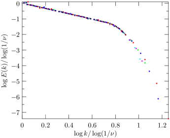
Figure 4: Collapse of the spectra in Fig. 1 with the rescaling proposed by Frisch and Vergassola.

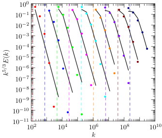
Figure 5: Intermediate dissipation ranges in the simulations of Fig. 1. For each case, the dots indicate the portion of the numerical spectrum for $k>1/\eta$, the solid line depicts the spectrum given by (26), and the vertical dashed line separates regions of equal energy dissipation.

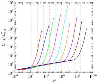
Figure 6: The rapid growth of the flux kurtosis for the simulations of Fig. 1 in each intermediate dissipation range, beginning at $k_{d}$ (denoted by a vertical dashed line).

In summary, we were able to determine the effective dimension $D(h)$ and study its effects on the dissipation-range energy spectrum. The steepening of the energy spectrum in the inertial range implies that the dissipation range sets in well after the Kolmogorov scale is reached, namely at the scale determined by (20) or (23). Frisch and Vergassola [21] note that this reduction in scale compared to the Kolmogorov scale is relatively small, but our numerical simulations are precise enough to resolve it.

5 Dissipation-scale effects on inertial-range dynamics

When the number of shells is kept fixed, and the viscosity is reduced, the viscous range will become narrower and narrower, until it finally disappears. Schörghofer et al. [42] call this the regime of strong interaction. However, as this happens, the effect of the lack of resolution no longer remains confined to the small scales: it begins to affect the inertial-range intermittency corrections as well. This effect is illustrated in Fig. 7 for simulations with fixed viscosity and varying $N$. In particular, we see on comparing the $N=18$ and $N=20$ spectra that it is necessary to resolve the small-scale dynamics well beyond the dissipation wavenumber $k_{d}$ (denoted by the vertical dashed line). The smallest number of shells for which the large-scale dynamics was adequately resolved was $N=20$, which requires a maximum wavenumber more than three times higher than $k_{d}$. For the case $N=14$, where the viscous range was completely resolved, it was necessary to use the conservative C–RK5 integrator described in Appendix B to discretize the nonlinear terms in a manner that respects exact energy conservation. Otherwise, as illustrated for the nonconservative solution in the transfer function inset, viscous dissipation will be insufficient to absorb the temporal energy discretization error, so that a global energy balance can never be reached. In Fig. 8, we use this conservative integrator to illustrate the eventual equipartition of shells energies and resulting $k^{-1}$ energy spectrum, in the extreme limit of zero dissipation, given an initial $k^{-2}$ spectrum.

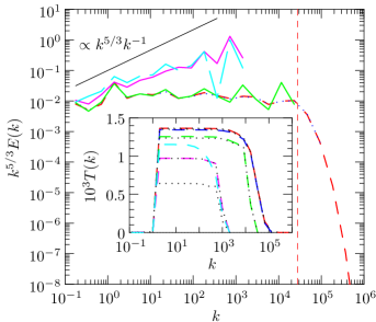
Figure 7: The effect of a finite number of shells on the spectrum for the standard case $(\beta=-1/2,\lambda=2)$ of Ref. [31]. For $N=26$ (dashed) and $N=20$ (dotted), there is no discernible difference between the energy spectra, showing that a sufficient number of shells in the viscous subrange is included. The vertical dashed line denotes the dissipation wavenumber $k_{d}$. For $N=18$ (solid), the dissipation range is barely resolved and the inertial range is contaminated. For $N=14$, the inertial range tends toward the statistical equipartition spectrum $k^{-1}$: the short solid curve indicates the spectrum obtained with a conservative integrator; the long-dashed curve indicates the spectrum obtained with a nonconservative exponential integrator that violates global energy balance.

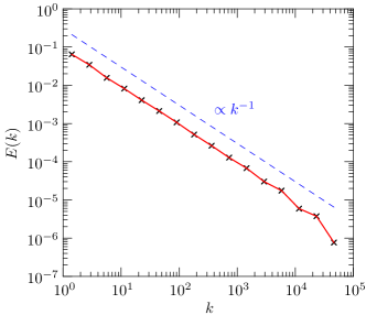
Figure 8: Equipartition spectrum for 16 shells obtained with the conservative C–RK5 integrator with $\epsilon=\nu=0$.

In view of these simulations, the conjecture in [42] on the role of preservation of the helicity $H$ has to be reconsidered. Kadanoff et al. noted that their simulations for the standard case $(\beta=-1/2,\lambda=2)$ closely reproduced experimentally measured intermittency exponents of three-dimensional turbulence (cf. Fig. 3). At the time, it had already been observed [5] that for fixed $\lambda$, the intermittency corrections strongly depend on the parameter $\beta$, as illustrated in Fig. 9. Kadanoff et al. then hypothesized that experimentally observed exponents should be obtained on the curve $\lambda=1/(1+\beta)$ along which the second conserved invariant of the GOY model is analogous to the helicity invariant of three-dimensional Navier–Stokes turbulence.

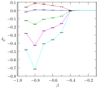
Figure 9: Scaling anomalies $\delta_{p}$, with $\lambda=2$, for $p=2$, $3$, $4$, $5$, and $6$ (from top to bottom) vs. $\beta$, as obtained by a least-squares fit between $k=500$ and $2\times 10^{6}$. The number of shells is $32$ and the viscosity $\nu$ is $10^{-11}$. The system is driven with a stochastic white-noise force on the first shell such that the energy injection $\epsilon=1$.

However, on repeating their simulation with a sufficient number of shells, (particularly the case with $\beta=-3/10$ and $\lambda=10/7$, which requires $44$ rather than $22$ shells), we find that the structure function exponents change dramatically. In particular, in view of Fig. 10, it appears that the distinction made between the cases with and without helicity conservation in Fig. 4 of Ref. [31] cannot be upheld: helicity preservation does not lead to unique intermittency corrections. This is further emphasized in Fig. 11, where the variation of the anomalies $\delta_{p}$ with $\beta$ along the helicity preserving curve is shown. Fig. 12 emphasizes that the computed slopes are well resolved, and independent of the fitting interval, particularly for small values of $\beta$ (corresponding to small $\lambda$ and large $N$), where the departure from the conjecture is seen to be most significant.

While Fig. 10 might appear to support the conjecture at least for $p=2$, we see that neither Fig. 11 nor the higher-resolution analog Fig. 13 of Fig. 10 generated using data from Figs. 9 and 11, agree with it. Our high-resolution numerical data set is sufficiently well resolved that we did not need to invoke extended self-similarity to obtain the results in Fig. 13.

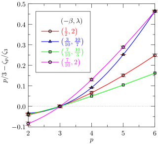
Figure 10: Recalculation of Fig. 4 from Kadanoff et al., fitting between $k=20$ and $200$. The first three $(-\beta,\lambda)$ pairs respect helicity conservation; the fourth does not. All four cases exhibit large anomalies, independent of whether helicity is preserved.

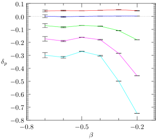
Figure 11: Scaling anomalies $\delta_{p}$ from top to bottom for $p=2$, $3$, $4$, $5$, and $6$ in the helicity-preserving case where $\lambda=1/(1+\beta)$ for the values of $\beta$ and number of shells $N$ listed in Table 2, as obtained by a least-squares fit between $k=500$ and $2\times 10^{6}$. The viscosity $\nu$ is $10^{-11}$. The system is driven with a stochastic white-noise force on the first shell such that the energy injection $\epsilon=1$.

Figure 12: Determination of $\delta_{6}$ from the logarithmic slope of $\Sigma_{n,6}$ for different values of $\beta$, with $\lambda=1/(1+\beta)$.

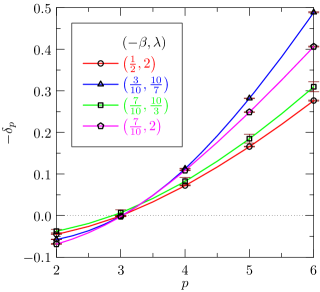
Figure 13: Analog of Fig. 10 generated from the high-resolution data in Figs. 9 and 11.

$\beta$	$-\frac{2}{10}$	$-\frac{3}{10}$	$-\frac{4}{10}$	$-\frac{1}{2}$	$-\frac{6}{10}$	$-\frac{7}{10}$
$\lambda$	$\frac{10}{8}$	$\frac{10}{7}$	$\frac{10}{6}$	$2$	$\frac{10}{4}$	$\frac{10}{3}$
$N$	$99$	$62$	$43$	$32$	$24$	$19$
$\delta_{2}$	$0.04$	$0.05$	$0.047$	$0.043$	$0.044$	$0.042$
$\delta_{4}$	$-0.18$	$-0.11$	$-0.08$	$-0.07$	$-0.08$	$-0.07$
$\delta_{6}$	$-0.75$	$-0.50$	$-0.30$	$-0.27$	$-0.32$	$-0.30$

Table 2: Values of $\beta$, $\lambda$, $N$, $\delta_{2}$, $\delta_{4}$, and $\delta_{6}$ for the helicity-preserving cases.

6 Conclusions

In this work, we exploited the numerical advantages of the GOY model, combined with efficient integration algorithms, to obtain fully converged spectra that allowed us to address links between dissipation, scaling, and conserved quantities.

We documented that the typical dissipation scale is much smaller than the Kolmogorov length, due to the inherent steepening of the spectrum by intermittency corrections. While the detailed form of the spectrum beyond this point is influenced by the probability distribution of the velocity scaling exponent, as discussed by Frisch and Vergassola [21], the delayed transition is not. Overall, the effect is relatively small, but easily identified in simulations of the GOY model.

The shell model simulations presented here also underscore the need to fully resolve the small scales. They demonstrate how insufficient resolution of the viscous subrange can affect inertial-range scaling exponents. In particular, when the viscous range is fully resolved, one observes significant variations in the spectral exponents even along the helicity preserving curve, thus disproving a previous conjecture [31]. For the standard case of Ref. [31], we found that the upper truncation wavenumber must be at least three times higher than the dissipation wavenumber $k_{d}$ in order to capture the proper inertial-range dynamics.

While current direct numerical simulations of three-dimensional Navier–Stokes turbulence barely reach into the inertial range, the implication of this relation between the second-order intermittency correction and the dissipation wavenumber is that, for future numerical simulations, it will become increasingly important to account properly for unresolved viscous scales.

Acknowledgements

We thank the Alexander von Humboldt Foundation, the Deutsche Forschungsgemeinschaft, the National Science and Engineering Research Council of Canada, the Pacific Institute for Mathematical Sciences, and the U.S. National Science Foundation for their generous support. This work was completed while BE was visiting the University of Maryland as Burgers Professor. It is a pleasure to thank the Burgers board and in particular Dan Lathrop for their hospitality at the University of Maryland. We also thank Sigfried Grossmann for discussions on the contents of section III and Andrew Hammerlindl and Tom Prince for their contributions to Asymptote (asymptote.sf.net), the descriptive vector graphics language used to draw the figures in this work.

Appendix A Exponential adaptive (3,2) Bogacki–Shampine Runge–Kutta integrator

The GOY model can be written as a set of ordinary differential equations for the components of the vector ${\bm{u}}=(u_{0},u_{1},\ldots,u_{N-1})$:

$$\frac{d{\bm{u}}}{dt}+{\bm{\nu}}{\bm{u}}=\bm{S}({\bm{u}}),$$ (27)

where ${\bm{\nu}}$ is a diagonal matrix with entries $(\nu k_{0}^{2},\nu k_{1}^{2},\ldots,\nu k_{N-1}^{2})$.

A general $s$-stage autonomous Runge–Kutta scheme that evolves an initial value ${\bm{u}}_{0}$ by a time step $\tau$ to a final value ${\bm{u}}_{s}$ may be written in the form

$${\bm{u}}_{i}={\bm{u}}_{0}+\tau\sum_{j=0}^{i-1}{\bm{a}}_{ij}\bm{S}({\bm{u}}_{j})\qquad(i=1,\ldots,s).$$ (28)

Letting ${\bm{x}}=-\tau{\bm{\nu}}$, the $4$-stage exponential Bogacki–Shampine Runge–Kutta order (3,2) embedded pair [11] uses the coefficients

$${\bm{a}}_{10} = \frac{1}{2}\varphi_{1}\left(\frac{1}{2}{\bm{x}}\right),$$

$${\bm{a}}_{20} = \frac{3}{4}\varphi_{1}\left(\frac{3}{4}{\bm{x}}\right)-a_{21},\ \ \ {\bm{a}}_{21}=\frac{9}{8}\varphi_{2}\left(\frac{3}{4}{\bm{x}}\right)+\frac{3}{8}\varphi_{2}\left(\frac{1}{2}{\bm{x}}\right),$$

$${\bm{a}}_{30} = \varphi_{1}({\bm{x}})-{\bm{a}}_{31}-{\bm{a}}_{32},\ {\bm{a}}_{31}=\frac{1}{3}\varphi_{1}({\bm{x}}),\ \ {\bm{a}}_{32}=\frac{4}{3}\varphi_{2}({\bm{x}})-\frac{2}{9}\varphi_{1}({\bm{x}}),$$

$${\bm{a}}_{40} = \varphi_{1}({\bm{x}})-\frac{17}{12}\varphi_{2}({\bm{x}}),\ \ {\bm{a}}_{41}=\frac{1}{2}\varphi_{2}({\bm{x}}),\ \ {\bm{a}}_{42}=\frac{2}{3}\varphi_{2}({\bm{x}}),\ \ {\bm{a}}_{43}=\frac{1}{4}\varphi_{2}({\bm{x}}),$$

where the (here diagonal) matrix functions $\varphi_{1}$ and $\varphi_{2}$ are given by $\varphi_{1}({\bm{x}})={\bm{x}}^{-1}(e^{\bm{x}}-\bm{1})$ and $\varphi_{2}({\bm{x}})={\bm{x}}^{-2}(e^{\bm{x}}-\bm{1}-{\bm{x}})$. The value ${\bm{u}}_{3}$ is the third-order solution, while the value ${\bm{u}}_{4}$ provides a second-order estimate that can be used to optimally adjust the time step. Since $\bm{S}({\bm{u}}_{3})$ is just the value of $\bm{S}$ at the initial ${\bm{u}}_{0}$ for the next time step, no additional source evaluation is actually required to compute ${\bm{u}}_{4}$ (unless an extra stochastic forcing term is added to ${\bm{u}}_{3}$ before proceeding to the next time step).

Care must be exercised when evaluating the diagonal components $\varphi_{1}(x)$ and $\varphi_{2}(x)$ near $0$; optimized double precision routines for evaluating these functions are available at www.math.ualberta.ca/$\sim$bowman/phi.h.

Appendix B Conservative adaptive (5,4) Runge–Kutta integrator

Here we describe a fifth-order conservative integrator (C–RK5) similar to the second-order conservative predictor–corrector algorithm introduced in [12, 44, 33]. We first consider the case where each component of ${\bm{u}}$ in (27) is real. The scheme shares the same first five stages as the classical $6$-stage Cash–Karp Fehlberg Runge–Kutta (4,5) embedded (RK5) pair. However, the final conservative stage is derived by applying the final conventional stage to the evolution equation for each (say, $r^{\rm th}$) component $u$ of ${\bm{u}}$:

$$\frac{du^{2}}{dt}=2\widetilde{S}({\bm{u}})u,$$ (29)

where $\widetilde{S}({\bm{u}})=\bm{S}_{r}({\bm{u}})-{\bm{\nu}}_{r}{\bm{u}}_{r}$. One then transforms the resulting estimate for the new value of $u^{2}$ back into an estimate for $u$. The conventional RK5 estimate can be used to resolve the appropriate branch of the square root:

$$u_{6}=\mathop{\rm sgn}\nolimits\Big{(}u_{0}+\tau\sum_{j=0}^{5}{\bm{a}}_{5j}\widetilde{S}({\bm{u}}_{j})\Big{)}\sqrt{u_{0}^{2}+2\tau\sum_{j=0}^{5}{\bm{a}}_{5j}\widetilde{S}({\bm{u}}_{j})u_{j}}.$$ (30)

In regions where the argument of the square root becomes negative, the time step needs to be temporarily reduced. The resulting solution is then compared with the conventional fourth-order estimate $u_{0}+\tau\sum_{j=0}^{5}{\bm{a}}^{\prime}_{5j}\widetilde{S}({\bm{u}}_{j})$ (for a second set of coefficients ${\bm{a}}^{\prime}_{5j}$) to adjust the time step appropriately. When $u$ is complex, one applies (30) separately to the real and imaginary parts of $u$.

The transfer function $\Pi_{M}$ is based on partial sums of the time averages of ${\mathcal{S}}_{n}u_{n}^{*}$ from time $t_{1}$ to $t_{2}$. We compute these time averages as $[T_{n}(t_{2})-T_{n}(t_{1})]/(t_{2}-t_{1})$, where

$$\frac{dT_{n}}{dt}={\mathcal{S}}_{n}u_{n}^{*}.$$ (31)

Energy conservation relies on the fact that $\sum_{n=0}^{N-1}T_{n}$ is invariant (since $\sum_{n=0}^{N-1}{\mathcal{S}}_{n}u_{n}^{*}=0$). Since integrators of the form (28) conserve such invariants that are linear in the evolved variable [33], one can use a conventional RK5 integrator to conservatively evolve (31).

We compute time averages of $u_{n}^{2}$ as $[M_{n}(t_{2})-M_{n}(t_{1})]/(t_{2}-t_{1})$, where

$$\frac{dM_{n}}{dt}=\left|u_{n}\right|^{2}.$$ (32)

Energy conservation implies that $\sum_{n=0}^{N-1}M_{n}$ should grow linearly with time; hence we must use conservative values of $u_{n}$ on the right-hand side of 32. Since we only compute conservative solutions $u_{n}$ at the beginning and the end of each time step, we are restricted to using a (second-order) trapezoidal rule to perform the integration of (32).

References

- [1] T. Bell and M. Nelkin, Nonlinear cascade models for fully developed turbulence, Phys. Fluids 20 (1977) 345–350.
- [2] R. Benzi, N. Horesh, and I. Procaccia, Shell model of two-dimensional turbulence in polymer solutions, Europhys. Lett. 68 (2004) 310–315.
- [3] G. Beylkin, J. M. Keiser, and L. Vozovoi, A new class of time discretization schemes for the solution of nonlinear PDEs, J. Comp. Phys. 147 (1998) 362–387.
- [4] L. Biferale, Shell models of energy cascade in turbulence, Annu. Rev. Fluid Mech. 35 (2003) 441–468.
- [5] L. Biferale, A. Lambert, R. Lima, and G. Paladin, Transition to chaos in a shell model of turbulence, Physica D 80 (1995) 105–119.
- [6] D. Biskamp, Cascade models for magnetohydrodynamic turbulence, Phys. Rev. E 50 (1994) 2702–2711.
- [7] G. Boffetta, A. Celani, and D. Roagna, Energy dissipation statistics in a shell model of turbulence, Phys. Rev. E 61 (2000) 3234–3236.
- [8] G. Boffetta and G. Romano, Structure functions and enery dissipation dependence on Reynolds number, Phys. Fluids 41 (2002) 3453–3458.
- [9] P. Bogacki and L. F. Shampine, A 3(2) pair of Runge-Kutta formulas, Appl. Math. Letters 2 (1989) 1–9.
- [10] T. Bohr, M. Jensen, G. Paladin, and A. Vulpiani, Dynamical systems approach to turbulence, Cambridge University Press, 1998.
- [11] J. C. Bowman and M. Roberts, An adaptive exponential integrator, J. Comp. Phys. (2006). to be submitted.
- [12] J. C. Bowman, B. A. Shadwick, and P. J. Morrison, Exactly conservative integrators, in 15th IMACS World Congress on Scientific Computation, Modelling and Applied Mathematics, A. Sydow, ed., vol. 2, Berlin, August 1997, Wissenschaft & Technik, 595–600.
- [13] J. Certaine, The solution of ordinary differential equations with large time constants, Math. Meth. Dig. Comp. (1960) 129–132.
- [14] L. Chevillard, B. Castaing, and E. Lévêque, On the rapid increase of intermittency in the near-dissipation range of fully developed turbulence, Eur. Phys. J. B 45 (2005) 561–567.
- [15] S. Cox and P. Matthews, Exponential time differencing for stiff systems, J. Comp. Phys. 176 (2002) 430–455.
- [16] J. Eggers and S. Grossmann, Does deterministic chaos imply intermittency in fully developed turbulence?, Phys. Fluids A 3 (1991) 1985.
- [17] J. Eggers and S. Grossmann, Effect of dissipation fluctuations on anomalous velocity scaling in turbulence, Phys. Rev. A 45 (1992) 2360.
- [18] A. Esser and S. Grossmann, Nonperturbative renormalization group approach to turbulence, Eur. Phys. J. B 7 (1999) 467–482.
- [19] G. Falkovich, Bottleneck phenomenon in developed turbulence, Phys. Fluids 6 (1994) 1411–1414.
- [20] U. Frisch, Turbulence: The legacy of A.N.Kolmogorov, Cambdridge University Press, 1995.
- [21] U. Frisch and M. Vergassola, A prediction of the multifractal model: the intermediate dissipation range, Europhys. Lett. 14 (1991) 439–444.
- [22] E. Gledzer, System of hydrodynamic type admitting two quadratic integrals of motion, Sov. Phys. Dokl. 18 (1973) 216.
- [23] S. Grossmann and D. Lohse, Scale resolved intermittency in turbulence, Phys. Fluids 6 (1994) 611.
- [24] S. Grossmann and D. Lohse, Universality in fully developed turbulence, Phys. Rev. E 50 (1994) 2784–2789.
- [25] S. Grossmann, D. Lohse, and A. Reeh, Developed turbulence: From full simulations to full mode reductions, Phys. Rev. Lett. 77 (1996) 5369–5372.
- [26] E. Hairer, S. Nørsett, and G. Wanner, Solving Ordinary Differential Equations II: Stiff and Differential-Algebraic Problems, vol. 14 of Springer Series in Comput. Math., Springer, Berlin, 1991.
- [27] J. Herweijer and W. van de Water, Universal shape of scaling functions in turbulence, Phys. Rev. Lett. 74 (1995) 4651–4654.
- [28] M. Hochbruck, C. Lubich, and H. Selfhofer, Explicit integrators for large systems of differential equations, SIAM J. Sci. Comput. 19 (1998) 1552–1574.
- [29] M. Hochbruck and A. Ostermann, Explicit exponential Runge-Kutta methods for semilinear parabolic problems, SIAM J. Numer. Anal. (2005). to appear.
- [30] M. Jensen, Shell model for turbulent advection of passive-scalar fields, Phys. Rev. A 45 (1992) 7214–7221.
- [31] L. P. Kadanoff, D. Lohse, J. Wang, and R. Benzi, Scaling and dissipation in the GOY shell model, Phys. Fluids 7 (1995) 617–629.
- [32] A. Kolmogorov, Local structure of turbulence in an incompressible viscous fluid at very large reynolds numbers, Dokl. Acad. Nauk SSSR 30 (1941) 299, reprinted in Proc. R. Soc. Lond. A (1991) 434, 9–13.
- [33] O. Kotovych and J. C. Bowman, An exactly conservative integrator for the -body problem, J. Phys. A.: Math. Gen. 35 (2002) 7849–7863.
- [34] E. Lévêque and C. R. Koudella, Finite-mode spectral model of homogeneous and isotropic Navier–Stokes turbulence: A rapidly depleted energy cascade, Phys. Rev. Lett. 86 (2001) 4033–4036.
- [35] E. Leveque and Z. She, Viscous effects on inertial range scaling in a dynamical model of turbulence, Phys. Rev. Lett. 75 (1995) 2690–2693.
- [36] D. Lohse and A. Müller-Groeling, Bottleneck effects in turbulence: scaling phenomena in r- versus p-space, Phys. Rev. Lett. 74 (1995) 1747–1750.
- [37] D. Lohse and A. Müller-Groeling, Anisotropy and scaling corrections in turbulence, Phys. Rev. E 54 (1996) 395–405.
- [38] Y. Nakayma, T. Watanabe, and H. Fujisaka, Self-similar fluctuation and large deviation statistics in the shell model of turbulence, Phys. Rev. E 64 (2001) 056304(1–13).
- [39] E. A. Novikov, Functionals and the random-force method in turbulence theory, J. Exptl. Theoret. Phys. (U.S.S.R) 47 (1964) 1919–1926.
- [40] K. Ohkitani and M. Yamada, Temporal intermittency in the energy cascade process and local Lyapunov analysis in fully developed model turbulence, Prog. Theor. Phys. 81 (1989) 329.
- [41] D. Pisarenko, L. Biferale, D. Courvoisier, U. Frisch, and M. Vergassola, Further results on multifractality in shell models, Phys. Fluids A 5 (1993) 2533–2538.
- [42] N. Schörghofer, L. P. Kadanoff, and D. Lohse, How the viscous subrange determines inertial range properties in turbulence shell models, Physica D 88 (1995) 40–54.
- [43] J. Schumacher, K. R. Sreenivasan, and P. K. Yeung, Very fine structures in scalar mixing, J. Fluid Mech. 531 (2005) 113–122.
- [44] B. A. Shadwick, J. C. Bowman, and P. J. Morrison, Exactly conservative integrators, SIAM J. Appl. Math. 59 (1999) 1112–1133.
- [45] Z. She and E. Leveque, Universal scaling laws in fully developed turbulence, Phys. Rev. Lett. 72 (1994) 336.
- [46] E. D. Siggia, Origin of intermittency in fully developed turbulence, Phys. Rev. A 15 (1977) 1730–1750.
- [47] M. Yamada and K. Ohkitani, Lyapunov spectrum of a chaotic model of three-dimensional turbulence, J. Phys. Soc. Jap. 56 (1987) 4210–4213.
- [48] M. Yamada and K. Ohkitani, The inertial subrange and non-positive Lyapunov exponents in fully developed turbulence, Prog. Theor. Phys. 79 (1988) 1265.
- [49] M. Yamada and K. Ohkitani, Lyapunov spectrum of a model of two-dimensional turbulence, Phys. Rev. Lett. 60 (1988) 983.