Effects of population mixing on the spread of SIR epidemics

Abstract

Abstract: - We study dynamics of spread of epidemics of SIR type in a realistic spatially-explicit geographical region, Southern and Central Ontario, using census data obtained from Statistics Canada, and examine the role of population mixing in epidemic processes. Our model incorporates the random nature of disease transmission, the discreteness and heterogeneity of distribution of host population.We find that introduction of a long-range interaction destroys spatial correlations very easily if neighbourhood sizes are homogeneous. For inhomogeneous neighbourhoods, very strong long-range coupling is required to achieve a similar effect. Our work applies to the spread of influenza during a single season.

I Introduction

Studies of some epidemics, for example, the spread of the Black Death in Europe from 1347–1350 Langer (1964), the past influenza pandemics Rvachev and Longini (1995), spread of fox rabies in Europe, or spread of rabies among raccoons in eastern United States and Canada Murray (2003), indicate that host and infective interactions and spatial distributions of their populations should play an important role in the dynamics of spread of many infectious diseases.

Until recently most mathematical models of spread of epidemics have described interactions of large number of individuals in aggregate form and often these models have neglected aspects of spatial distribution of populations, importance of which have been addressed in Durret and Levin (1994). Adopting methodologies like cellular automata, coupled map lattices, lattice gas cellular automata or agent based simulations, new classes of models have been proposed and studied Fukś and Lawniczak (2001); Di Stefano et al. (2000); Benyoussef et al. (1999); Fukś et al. (2005); Watts (2004); Barrett et al. (2005), to incorporate with various levels of abstraction and details: direct interactions among individuals; spatial distribution of population types (i.e., infective, susceptible, removed); individuals’ movement; effects of social networks on spread of epidemics.

The goal of our work is to study the effects of population interactions and mixing on the spatio-temporal dynamics of spread of epidemics of SIR (susceptible-infected-removed) type in a realistic population distribution. For the purpose of our study we developed a fully discrete individually-based simulation model that incorporates the random nature of disease transmission. The key feature of this model is the fact that for each individual the set of all individuals with whom he/she interacts may change with time. This results in time varying small world network structure.

As a case study we considerder census data obtained from Statistic Canada Statistics Canada (2001a, b) for Southern and Central Ontario. The data set specifies population of small areas composed of one or more neighbouring street blocks, called “dissemination areas”. Using these data, we study the effects of two types of interactions among individuals on the spread of epidemics. The first type of interaction is the one among individuals located only in adjacent dissemination areas. The second type of interaction is the one among individuals who in addition to being in contact with members of their own and adjacent dissemination areas may also be in contact with individuals located in remote, non adjacent, dissemination areas. This last case can be seen as a case of ”short-cuts” among multiple far away dissemination areas. We investigate spatial correlations in our model and how they can be destroyed by the ”short-cuts” in population contacts. Additionally, we derive a mean field description of our individually based simulation model and compare the results of the two models.

The presented work is continuation and expansion of our work in Fukś and Lawniczak (2001); Di Stefano et al. (2000); Fukś et al. (2005) and contributes to better understanding of spread of epidemics of SIR type, including influenza.

II SIR epidemic model description

In order to study how population interactions (”population mixing”) affects the spread of epidemics we construct an individually based model in which each individual is represented by a particle, as in our earlier work Fukś and Lawniczak (2001); Di Stefano et al. (2000). Models of this type take various forms, ranging from stochastic interacting particle systems Durret and Levin (1994) to models based on cellular automata or coupled map lattices Schönfisch (1993); Boccara and Cheong (1993); Duryea et al. (1999); Benyoussef et al. (1999).

In our model, we consider a set of $N$ individuals, labelled with consecutive integers $1,2\ldots,N$. This set of labels is denoted by $\mathcal{L}$. We assume that each individual, at any given time can be in one of three, mutually exclusive, distinct states: susceptible (S), infected (I) or removed (R). An individual can change state only in two ways: a susceptible individual who comes in direct contact with an infected individual can become infected with probability $p$; an infected individual can become removed with probability $q$. The precise description of the model is as follows.

The state of the $i$-th individual at the time step $k$ is described by a Boolean vector variable $\boldsymbol{\eta}(i,k)=\langle\eta_{S}(i,k),\eta_{I}(i,k),\eta_{R}(i,k)\rangle$, where $\eta_{\tau}(i,k)=1$ if the $i$-th individual is in the state $\tau$, where $\tau\in\{S,I,R\}$, and $\eta_{\tau}(i,k)=0$ otherwise. Thus,

$$\eta_{S}(i,k)\oplus\eta_{I}(i,k)\oplus\eta_{R}(i,k)=1.$$

We assume that $i=1,2,\ldots,N$ and $k\in\mathbb{N}$, that is, the time is discrete. Hence, the only allowed values of the vector $\boldsymbol{\eta}(i,k)$ are

$$\boldsymbol{\eta}(i,k)=\left\{\begin{array}[]{c}\langle 1,0,0\rangle,\text{ \ \ \ \ \ \ \ if the }i\text{\ -th individual's state }\in S\\ \langle 0,1,0\rangle,\text{ \ \ \ \ \ \ \ \ \ if the }i\text{\ -th individual's state }\in I\\ \langle 0,0,1\rangle,\text{ \ \ \ \ \ \ \ \ if the }i\text{\ -th individual's state }\in R\end{array}\right..$$

No other values of $\boldsymbol{\eta}(i,k)$ are possible in SIR epidemic model. In SIR model an individual can only be at one state at any give time and transitions occur only from susceptible to infected and from infected to removed. A removed individual does not become susceptible or infected again in SIR model. Therefore, SIR model is suitable for studying spread of influenza in the same season because the same type of influenza virus can infect an individual only once and once the individual is recovered from the flu it becomes immune to this type of virus.

We further assume that at time step $k$ the $i$-th individual can interact with individuals from a subset of $\mathcal{L}$, to be denoted by $C(i,k)$. Using this notation, after one time iteration the $\eta_{\tau}(i,k+1)$ becomes

$$\eta_{S}(i,k+1) = \eta_{S}(i,k)\prod_{j\in C(i,k)}(1-X_{i,j,k}\eta_{I}(j,k)),$$ (1)

$$\eta_{I}(i,k+1) = \eta_{S}(i,k)\left(1-\prod_{j\in C(i,k)}(1-X_{i,j,k}\eta_{I}(j,k))\right)+\eta_{I}(i,k)(1-Y_{i,k}),$$ (2)

$$\eta_{R}(i,k+1) = \eta_{R}(i,k)+\eta_{I}(i,k)Y_{i},$$ (3)

where $X=\{X_{i,j,k}:i,j=1,...,N$ and $k=1,2,....\}$ is a sequence of iid Boolean random variables such that $Pr(X_{i,j,k}=1)=p$, $Pr(X_{i,j,k}=0)=1-p$, and $Y=\{Y_{i,k}:i=1,...,N,$ and $k=1,2,...\}$ is a sequence  of iid Boolean variables such that $Pr(Y_{i}=1)=q$, $Pr(Y_{i}=0)=1-q$. We assume that the sequences $X$ and $Y$ of random variables are independent of each other and of the random variables $\eta_{\tau}(i,k).$

Observe that, if the $i$-th individual interacts with an infected $j$-th individual at time step $k$ and $X_{i,j,k}=1,$ then the infection is transmitted from the $j$-th individual to the $i$-th individual at this time step. Thus, if some product $X_{i,j,k}\eta_{I}(j,k)$ takes the value 1, then $\eta_{S}(i,k+1)=0$, meaning that the $i$-th individual has changed its state from susceptible to infected.

The key feature of this model is the set $C(i,k)$, representing all individuals with whom the $i$-th individual may have interacted at time step $k$. In a large human population, it is almost impossible to know $C(i,k)$ for each individual, so we make some simplifying assumptions. First of all, it is clear that the spatial distribution of individuals must be reflected in the structure of $C(i,k)$. We have decided to use realistic population distribution for Southern and Central Ontario using census data obtained from Statistic Canada Statistics Canada (2001a, b). The selected region is mostly surrounded by waters of Great Lakes, forming natural boundary conditions. The data set specifies population of so called “dissemination areas” , that is, small areas composed of one or more neighbouring street blocks. We had access to longitude and latitude data with accuracy of roughly $0.01^{\circ}$, hence some dissemination areas in densely populated regions have the same geographical coordinates. We combined these dissemination areas into larger units, to be called “modified dissemination areas” (MDA).

We now define the set $C(i,k)$ using the concept of MDAs. This set is characterized by two positive integers $n_{c}$ and $n_{f}$. Let us label all MDAs in the region we are considering by integers $m=1,2,\ldots,M$, where in our case $M=5069$. For the $i$-th individual belonging to the $m$-th MDA, the set $C(i,k)$ consists of all individuals belonging to the $m$-th MDA plus all individuals belonging to the $n_{c}$ MDAs nearest to the $m$-th MDA and the $n_{f}$ MDAs randomly selected among all remaining MDAs. While the “close neighbours”, that is, the $n_{c}$ nearest MDAs, will not change with time, the “far neighbours”, that is, the $n_{f}$ randomly selected MDAs, will be randomly reselected at each time step.

III Derivation of mean field equations

The model described in the previous section involves strong spatial coupling between individuals. Before we describe consequences of this fact, we first construct a set of equations which approximate dynamics of the model under the assumption of “perfect mixing”, in other words, neglecting the spatial coupling.

The state of the system described by eq. (1–3) at time step $k$ is determined by the states of all individuals and is described by the Boolean random field $\boldsymbol{\eta}(k)=\{\boldsymbol{\eta}(i,k):i=0,\ldots,N\}$. Under the assumptions of our model, the Boolean field $\{\boldsymbol{\eta}(k):i=0,1,2\ldots\}$ is a Markov stochastic process.

By taking the expectation $E_{\boldsymbol{\eta}(0)}$ of this Markov stochastic process when the initial configuration is $\boldsymbol{\eta}(0)$ we get the probabilities of the $i$-th individual being susceptible, or infected, or removed at time $k$, that is, $\rho_{\tau}(i,k)=E_{\boldsymbol{\eta}(0)}\left[\eta_{\tau}(i,k)\right]$ for $\tau\in\{S,I,R\}$.

Since the sequences of random variables $X$ and $Y$ are independent of each other and of the sequences of the random variables $\eta_{\tau}(i,k)$, assuming additionally independence of random variables $\eta_{\tau}(i,k)$, the expected value of a product of these variables is equal to the product of expected values. Under these mean field assumptions, taking expected values of both sides of equations (1–3) we obtain

$$\rho_{S}(i,k+1) = \rho_{S}(i,k)\prod_{j\in C(i,k)}(1-p\rho_{I}(j,k)),$$ (4)

$$\rho_{I}(i,k+1) = \rho_{S}(i,k)\Big{(}1-\prod_{j\in C(i,k)}(1-p\rho_{I}(j,k))\Big{)}+\rho_{I}(i,k)(1-q),$$ (5)

$$\rho_{R}(i,k+1) = \rho_{R}(i,k)+\rho_{I}(i,k)q.$$ (6)

Since mean field approximations neglect spatial correlations, we further assume that $\rho_{\tau}(i,k)$ is independent of $i$, that is $\rho_{\tau}(i,k)=\rho_{\tau}(k)$. Even though sets $C(i,k)$ have different number of elements for different $i$ and $k$, for the purpose of this approximate derivation we assume that they all have the same number of elements $(1+n_{c}+n_{f})D$, where $D$ is the average MDA population. All these assumptions lead to

$$\rho_{S}(k+1) =\rho_{S}(k)(1-p\rho_{I}(k))^{(1+n_{c}+n_{f})D},$$ (7)

$$\rho_{I}(k+1) =\rho_{I}(k)+\rho_{S}(k)-\rho_{S}(k)(1-p\rho_{I}(k))^{(1+n_{c}+n_{f})D}-q\rho_{I}(k),$$ (8)

$$\rho_{R}(k+1) =\rho_{R}(k)+q\rho_{I}(k).$$ (9)

The third equation in the above set is obviously redundant, since $\rho_{S}(k)+\rho_{I}(k)+\rho_{R}(k)=1$.

Similarly to the classical Kermack-McKendrick model, mean field equations (7)-(9) exhibit a threshold phenomenon. Depending on the choice of parameters, we can have $\rho_{I}(k)<\rho_{I}(0)$ for all $k$, meaning that the infection is not growing and eventually it will die out because in our model no new individuals are being born or arrive from outside the area under consideration during the time of the epidemic. Alternatively, we can have $\rho_{I}(k)>\rho_{I}(0)$ for some $k$, meaning that the epidemic is spreading. The intermediate scenario of constant $\rho_{I}(k)$ will occur when $\rho_{I}(k)=\rho_{I}(0)$, that is, when

$$\rho_{S}(0)-\rho_{S}(0)(1-p\rho_{I}(0))^{(1+n_{c}+n_{f})D}-q\rho_{I}(0)=0.$$ (10)

Assuming that initially the entire population consists only of susceptible and infective individuals, that is, there are no individuals in the removed group at $k=0,$we have $\rho_{S}(0)=1-\rho_{I}(0)$. Furthermore, if $(1+n_{c}+n_{f})D$ is large, we can assume $(1-p\rho_{I}(0))^{(1+n_{c}+n_{f})D}\approx 1-p(1+n_{c}+n_{f})D\rho_{I}(0)$. Solving eq. (10) for $q$ under these assumptions we obtain

$$q=\Big{(}1-\rho_{I}(0)\Big{)}(1+n_{c}+n_{f})Dp.$$ (11)

Thus, assuming the mean field approximation the epidemic can occur only if $q<\Big{(}1-\rho_{I}(0)\Big{)}(1+n_{c}+n_{f})Dp$.

IV Spatio-temporal dynamics of SIR epidemic model

The mean-field equations derived in the previous section depend only on the sum of $n_{c}$ and $n_{f}$. This means, for example, that the model with $n_{c}=12$, $n_{f}=0$ and the model with $n_{c}=11$, $n_{f}=1$ will have the same mean field equations. However, the actual dynamics in these two cases are very different, see Figure 2 and Figure 4. Depending on the relative size of $n_{f}$ and $n_{c}$, the epidemic may propagate or die out, as the following analysis shows. In order to make the subsequent analysis more convenient, we introduce parameter $\gamma$, defined as

$$\gamma=\frac{n_{f}}{n_{c}+n_{f}}.$$ (12)

Let $N_{\tau}(k)$ be the expected value of the total number of individuals belonging to class $\tau\in\{S,I,R\}$, that is,

$$N_{\tau}(k)=E_{\boldsymbol{\eta}(0)}\left(\sum_{i=1}^{N}\eta_{\tau}(i,k))\right)=\sum_{i=1}^{N}\rho_{\tau}(i,k).$$

We say that an epidemic occurs if there exists $k>0$ such that $N_{I}(k)>N_{I}(0)$. For fixed $p$, $n_{f}$ and $n_{c}$, there exists a threshold value of $q$ to be denoted by $q_{c}$, such that for each $q<q_{c}$ an epidemic occurs, and for $q>q_{c}$ it does not occur. Obviously $q_{c}$ depends on $p$, and this is illustrated in Figure 1, which shows graphs of $q_{c}$ as a function of $p$ for several different values of $\gamma$, where $n_{f}+n_{c}=12$. The graphs were obtained numerically by direct computer simulations of the model. The condition $n_{f}+n_{c}=12$ means that the size of the neighbourhood is kept constant, but the proportion of “far neighbours” (represented by $\gamma$) varies.

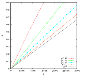
Figure 1: Graphs of critical lines for $\gamma=0.42,0.75,0.92$, and $1.0$. The first line from the bottom represents mean field approximation.

Figure 1 also shows the mean-field line given by eq. (11).

We observe that the parameter $\gamma$ controls dynamics of the epidemic process in a significant way, shifting the critical line up or down. When $\gamma=0$, that is, when there are no interactions with “far neighbours”, the epidemic process has a strictly local nature, and we can observe well defined epidemic fronts propagating in space, regardless at which MDA the epidemic starts at $k=0$. This is illustrated in Figure 2, where the epidemic starts at a single centrally located MDA with low population density (Figure 2a) and on Figure 3, where the epidemic starts in a MDA with high population density (Figure 3a). The simulations were done for the same parameters in both cases except for the different locations of the onsets of epidemics. The figures display MDAs that are represented by pixels colored according to the density of individuals of a given type. The red component of the color represents density of infected individuals, green density of susceptibles, and blue density of removed individuals. By density we mean the number of individuals of a given type divided by the size of the population of the MDA.

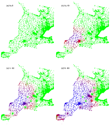
Figure 2: Example of a propagating epidemic front for $\gamma=0$, $p=0.00005$, $q=0.05$, with (a) $k=0$, (b) $k=40$, (c) $k=60$ and (d) $k=80$. The initial outbreak is located in an area with low population density. Modified dissemination areas are represented by pixels colored according to density of individuals of a given type, such that the red component represents density of infected, green density of susceptibles, and blue density of removed individuals.

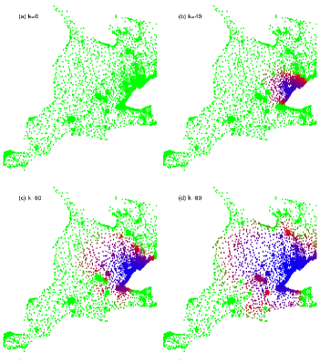
Figure 3: Example of a propagating epidemic front parameters identical as in Figure 2, except that the initial outbreak is now located in an area with high population density. Color coding like in the previous figure.

The epidemic waves propagating outwards can be clearly seen on Figure 2 and Figure 3, in the successive snapshots (b), (c) and (d). The fronts are mostly red. This means that the bulk of infected individuals is located at the fronts. After these individuals gradually recover the centers become blue.

Let us now consider slightly modified parameters, taking $\gamma=\frac{1}{12}$. This means that we now replace one “close” MDA by one “far” MDA. This does not seem to be a significant change, yet the effect of this change is truly noticeable.

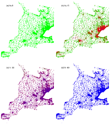
Figure 4: Development of the epidemic for $\gamma=\frac{1}{12}$, $p=0.00005$, $q=0.05$, with (a) $k=0$, (b) $k=15$, (c) $k=30$ and (d) $k=60$. Colour coding is the same as in the previous figure.

As we can see in Figure 4, the epidemic propagates much faster, and there are no visible fronts. The disease quickly spreads over the entire region and large metropolitan areas become red in a short time, as shown in Figure 4(b). This suggests that infected individuals are more likely to be found in densely populated regions, and their distribution is dictated by the population distribution – unlike in Figure 2 or Figure 3, where infected individuals are to be found mainly at the propagating front.

V Spatial correlations of SIR epidemic model

In order to quantify the observations of the previous section, we use a spatial correlation function for densities of infected individuals defined as

$$h(r,k)=\left\langle\eta_{I}(i,k)\eta_{I}(j,k)\right\rangle_{r\leq d(i,j)\leq r+\Delta r},$$

where $d(i,j)$ is the distance between $i$-th and $j$-th individual, and $<\cdot>$ represents averaging over all pairs $i$, $j$ satisfying condition $r\leq d(i,j)\leq r+\Delta r$. In the following considerations we take $\Delta r=1\,\mathrm{km}$. The distance between two individuals is defined as the distance between MDAs to which they belong.

Consider now a specific example of the epidemic process described by eq. (1-3), where $p=0.000015$, $q=0.2$, and $n_{c}+n_{f}=12$. For this choice of parameters epidemics always occur as long as $\gamma>0$. Figure 5 shows graphs of the correlation functions $h(r,k_{max})$ at the peak of each epidemic, so that $k_{max}$ is the time step at which the number of infected individuals achieves its maximum value.

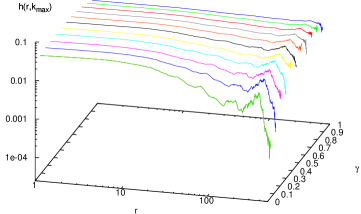
Figure 5: Graphs of the correlation function $h(r,k_{max})$ for different values of $\gamma$, where $p=0.000015$, $q=0.2$, and $n_{c}+n_{f}=12$.

An interesting phenomenon can be observed in the figure under consideration: while the increase of the proportion of “far” neighbours does destroy spatial correlations, one needs very high proportion of “far”neighbours to make the correlation curve completely flat. In Bonabeau et al. (1998) it is reported that for influenza epidemics $h(r,k_{max})\sim r^{0.04\pm 0.03}$. If we fit $h(r,k_{max})=Cr^{\alpha}$ curve to the correlation data shown in Figure 5, we obtain values of the exponent $\alpha$ as shown in Figure 6. In order to obtain $\alpha$ of comparably small magnitude as reported in Bonabeau et al. (1998), one would have to take $\gamma$ equal to at least $0.83$, meaning that vast majority of neighbours would have to be “far neighbours”.

Figure 6: Values of the exponent $\alpha$ for different values of the parameter $\gamma$. The exponent has been obtained by fitting $h(r,k_{max})=Cr^{\alpha}$ to simulation data.

In reality, this would require that the vast majority of all individuals one interacted with were not his/her neighbours, coworkers, etc., but individuals from randomly selected and possibly remote geographical regions. This is clearly at odds with our intuition regarding social interactions, especially outside large metropolitan areas. This prompted us to investigate further and to find out what is responsible for this effect.

Upon closer examination of spatial patterns generated in simulations of our individually-based model, we reach the conclusion that the inhomogeneity of population sizes in neighbourhoods $C(i,k)$ makes spatial correlations so persistent. Since different MDAs have different population sizes, we expect that some individuals will have larger neighbourhood populations than others, and as a result they will be more likely to get infected, even if the proportion of infected individuals is the same in all MDAs. This will build up clusters of infected individuals around populous MDAs.

To test if this is indeed the factor responsible for strong spatial correlations in our model, we replaced all MDA population sizes with a constant population size $D$, that is, the average MDA population size. As expected, graphs of the correlation functions obtained in this case were are all essentially flat, with the exponent $\alpha$ close to zero even in the case of $n_{f}=1$, when we obtained $\alpha=0.023\pm 0.002$.

VI Conclusions

We conclude that spatial correlations are difficult to destroy if neighbourhood sizes are inhomogeneous. Very significant amount of long-range interactions (i.e., very strong mixings) is required to obtain flat correlations curves. However, for homogeneous neighbourhood sizes, even relatively small long-range interaction immediately forces the process into the perfect-mixing regime, resulting in the lack of spatial correlations. The model that we developed can be applied to other realistic population distributions and geographical regions.

Acknowledgement

Henryk Fukś and Anna T. Lawniczak acknowledge partial financial support from the Natural Science and Engineering Research Council (NSERC) of Canada.

References

- Langer (1964) W. L. Langer, Scientific American pp. 114–121 (1964).
- Rvachev and Longini (1995) L. A. Rvachev and I. M. Longini, Mathematical Biosciences 75, 3 (1995).
- Murray (2003) J. D. Murray, Mathematical Biology II: Spatial Models and Biomedical Applications (Springer Verlag, New York, 2003).
- Durret and Levin (1994) R. Durret and S. Levin, Theoretical Population Biology 46, 363 (1994).
- Fukś and Lawniczak (2001) H. Fukś and A. T. Lawniczak, Discrete Dynamics Dynamics in Nature and Society 6, 191 (2001), eprint arXiv:nlin.CG/0207048.
- Di Stefano et al. (2000) B. Di Stefano, H. Fukś, and A. T. Lawniczak, in Proceedings of Canadian Conference on Electrical and Computer Engineering, Halifax, May 2000 (2000), pp. 26–31.
- Benyoussef et al. (1999) A. Benyoussef, N. Boccara, H. Chakib, and H. Ez-Zahraouy, Int. J. Mod. Phys. C 10, 1025 (1999).
- Fukś et al. (2005) H. Fukś, R. Duchesne, and A. Lawniczak, in Proceeding of 7th WSEAS International Conference on Applied Mathematics, Canun, Mexico, May 11-14 2005 (2005), pp. 108–113, eprint arXiv:nlin.CG/0505044.
- Watts (2004) D. J. Watts, Six Degrees: The Science of a Connected Age (W. W. Norton, 2004).
- Barrett et al. (2005) C. L. Barrett, S. G. Eubank, and J. P. Smith, Scientific American 292, 54 (2005).
- Statistics Canada (2001a) Statistics Canada, Dissemination area digital cartographic file, Statistics Canada, Geography Division, Ottawa, ON (2001a).
- Statistics Canada (2001b) Statistics Canada, Profile of age and sex, for Canada, provinces, territories, census divisions, census subdivisions, and dissemination areas, 2001 census, Industry Canada, Ottawa, ON (2001b).
- Schönfisch (1993) B. Schönfisch, Ph.D. thesis, Universität Tübingen (1993).
- Boccara and Cheong (1993) N. Boccara and K. Cheong, J.Phys. A: Math. Gen. 26, 3707 (1993).
- Duryea et al. (1999) M. Duryea, T. Caraco, G. Gardner, W. Maniatty, and B. K. Szymanski, Physica D 132, 511 (1999).
- Bonabeau et al. (1998) E. Bonabeau, L. Toubiana, and A. Flahault, J. Phys. A: Math. Gen. 31, L361 (1998).