Energy Transfer and Bottleneck Effect in Turbulence

Abstract

Past numerical simulations and experiments of turbulence exhibit a hump in the inertial range, called the bottleneck effect. In this paper we show that sufficiently large inertial range (four decades) is required for an effective energy cascade. We propose that the bottleneck effect is due to the insufficient inertial range available in the reported simulations and experiments. To facilitate the turbulent energy transfer, the spectrum near Kolmogorov’s dissipation wavenumber has a hump.

I Introduction

Energy spectrum of turbulent flow is an important quantity. In 1941, Kolmogorov K41a showed that the energy spectrum $E(k)$ of turbulent flow is

$$E(k)=K_{Ko}\Pi^{2/3}k^{-5/3}f(k/k_{d}),$$ (1)

where $\Pi$ is the energy flux, $K_{Ko}$ is Kolmogorov’s constant, $k_{d}$ is Kolmogorov’s wavenumber, and the function $f(x)\rightarrow 1$ in the inertial range ($x\ll 1$), and $f(x)\rightarrow 0$ as $x\gg 1$. Many experiments and numerical simulations verify this powerlaw apart from a very small intermittency correction. The compensated energy spectrum $E(k)k^{5/3}/K_{Ko}$ is flat in the inertial range, and decays in the dissipation range. A careful observation of energy spectrum obtained from recent high-resolution numerical simulations and experiments however show a small hump near Kolmogorov’s wavenumber $k_{d}$. The feature is called the bottleneck effect in literature. In this paper we propose an explanation for the bottleneck effect.

The bottleneck effect has been reported in many numerical simulations and experiments of fluid turbulence. Yeung and Zhou YeunZhou , Gotoh et al. Goto:VeloStat , Kaneda et al. Kane:Bottle , and Dobler et al. Bran:Bottle found the bottleneck effect (hump in the normalized energy spectrum) in their numerical simulations. Saddoughi and Veeravalli Veer:Bottle studied the energy spectrum of atmospheric turbulence and reported the bottleneck effect. They observed that the longitudinal spectra have a larger inertial range (around 1.5 decade) but smaller hump, while the transverse spectra have relatively smaller inertial range (around one decade), but a larger hump. Shen and Warhaft Shen , Pak et al. Pak:Bottle , She and Jackson She:Bottle , and other experimental groups also observed the bottleneck effect in fluid turbulence.

The bottleneck effect has been seen in other forms of turbulence as well. Watanabe and Gotoh and others Gotoh:Scalar_Bottle ; Yeung:JFM96 ; DonzKRS:Scalar reported the bottleneck effect in scalar turbulence, Haugen et al. Bran:Flux in three-dimensional magnetohydrodynamics, Biskamp et al. Bisk:Bottle_2D in two-dimensional magnetohydrodynamics, electron-magnetohydrodynamics, and thermal convection. Lamorgese et al. Pope:Hypervisc_Bottle , Biskamp et al. Bisk:Bottle_2D , and Dobler et al. Bran:Bottle observed that the bottleneck effect became more pronounced when hyperviscosity is increased.

There have been various attempts to explain bottleneck effect. Falkovich Falk:Bottleneck argued that the viscous suppression of small-scale modes removes some triads from nonlinear interactions, thus making it less effective, which leads to pileup of energy in the inertial interval of scales. Based on turbulent viscosity and the assumption of local energy transfer, Falkovich derived the following formula for the correction in Kolmogorov’s spectrum:

$$\delta E(k)=E(k)(k/k_{p})^{4/3}/\ln(k_{p}/k),$$ (2)

where $k_{p}$ is proportional to the dissipative wavenumber $k_{d}$, and $k\ll k_{p}$.

Yakhot and Zakharov YakhZakh:Cleb derived energy spectrum using Clebsch variables and showed that the energy spectrum is

$$E(k)=K_{Ko}\Pi^{2/3}k^{-5/3}f(k/k_{d})+Pk^{-1},$$ (3)

i.e., correction is of the form $k^{-1}$. Theoretical justification for $k^{-1}$ was argued by Orszag Orsz:Rev who analyzed the one-loop Dyson equation for the propagator $G$ and the velocity correlation function $U$; the spectrum $k^{-1}$ was obtained by assuming that the response function is dominated by viscous effects. She and Jackson She:Bottle reported an experimental result in which they observed the $k^{-1}$ bottleneck correction; they argued coherent vortex structures to be the reason for the bottleneck effect.

Kurien et al. Kuri:Bottle extended Kolmogorov’s phenomenology to include the effects of helicity. They found a shallower $k^{-4/3}$ energy spectrum at higher wavenumbers by assuming that the helicity transfer time-scales dominate at large wavenumbers. In the following discussion we will propose a new mechanism to explain the bottleneck effect. We argue that the bottleneck effect is seen when the length of inertial range is insufficient for the energy cascade process.

II The Reason for the Bottleneck Effect

The basic idea presented in our paper is as follows: In a fully-developed turbulence, a flux of energy is transferred from small wavenumbers to large wavenumbers. This process involves interactions of large number of modes—from small wavenumbers to large wavenumbers. The maximum energy transfer from a given wavenumber shell is to its nearest neighbour. Still significant amount of energy transfer takes place between somewhat distant wavenumber shells Krai:71 ; Zhou:Local ; Zhou:RevLocal ; Doma:Local2 ; Wale ; Ayye . Verma et al. Ayye showed using a theoretical arguments that if the inertial-range shells are divided in such a way that the $m$th shell is given by $k_{0}(2^{m/4}:2^{(m+1)/4})$, then in the inertial-range, the normalized shell-to-shell energy transfer rates from shell $m$ to shell $m+1,m+2,m+3$ are $18\%,6.7\%,$ and $3.6\%$ respectively. The remaining portion of energy flux, which is a huge fraction ($\sim$$70\%$), is transferred to the distant shells. This result is in agreement with earlier simulation results Zhou:Local .

The above arguments imply that for an effective cascade of energy, there must be a large enough range of wavenumbers. Ideally, when Kolmogorov’s wavenumber $k_{d}\rightarrow\infty$, Kolmogorov’s cascade is setup, and the energy spectrum is given by Eq. (1). However, if Kolmogorov’s wavenumber is not sufficiently large, the cascade process faces difficulty; at higher wavenumbers there are not enough number of modes to receive the energy transferred from the smaller wavenumbers. To compensate, the wavenumbers near Kolmogorov’s scale have a higher energy level. We propose this to be the main reason for the bottleneck effect. Note that the energy fed at small wavenumbers fixes the level of energy spectrum in the inertial range, and the energy input has to be dissipated at the higher wavenumbers. In the following discussion we will present a quantitative arguments to support the above idea.

II.1 Formalism

The average energy flux from a wavenumber sphere of radius $k_{0}$ is given by Lesi:book ; Lesl:book ; MKV:PR

$$\Pi(k_{0})=\int_{k>k_{0}}d\mathbf{k}\int_{p<k_{0}}d\mathbf{p}\left\langle S(k|p|q)\right\rangle$$ (4)

where $S(k|p|q)$ is the “mode-to-mode energy transfer rate” in a triad (p,q,k) with $\mathbf{k}=\mathbf{p+q}$, and $\left\langle\right\rangle$ represents the ensemble average. The term $S(k|p|q)$ represents the energy transfer rate from mode $\mathbf{p}$ to mode $\mathbf{k}$ with mode q acting as a mediator. The term $\left\langle S(k|p|q)\right\rangle$ has been computed earlier using standard field-theoretic technique Lesi:book ; Lesl:book ; McCoWatt ; McCo:book ; MKV:PR . The procedure to compute $\Pi(k_{0})$ is described in the above references, which yields

$$\Pi(k_{0})=K_{Ko}^{3/2}\Pi\left[\int_{k_{0}}^{\infty}dkk{}^{2}\int_{0}^{k_{0}}dp\int_{|k-p|}^{k+p}dq\frac{{pq}}{4k}\frac{{T_{1}C(p)C(q)+T_{2}C(q)C(k)+T_{3}C(p)C(k)}}{\nu^{*}(k^{2/3}+p^{2/3}+q^{2/3})}\right],$$ (5)

where $\nu^{*}$ is the renormalized parameter in the expression of renormalized viscosity McCoWatt ; McCo:book ; MKV:PR , and it has been found it to be between 0.35 to 0.40. In this paper we take $\nu^{*}=0.38$ MKV:PR . The correlation function $C(k)$ is related to the one-dimensional energy spectrum $E(k)$:

$$C(k)=\frac{{E(k)}}{4\pi k^{2}},$$ (6)

and $T_{i}^{\prime}$s are given in MKV:PR

$$T_{1} = kp(xy+2z^{3}+2xyz^{2}+x^{2}z),$$

$$T_{2} = -kp(xy+2z^{3}+2xyz^{2}+y^{2}z),$$

$$T_{3} = -kq(xz-2xy^{2}z-y^{2}z),$$

where $x,y,z$ are cosines defined as

$$\mathbf{p}\cdot\mathbf{q}=-pqx,\hskip 28.45274pt\mathbf{q}\cdot\mathbf{k}=qky,\hskip 28.45274pt\mathbf{p}\cdot\mathbf{k}=pkz.$$ (7)

The field-theoretic method mentioned above has certain similarities with the calculations based on the eddy-damped quasi-normal Markovian approximation (EDQNM). Both these methods use quasi-normal approximation, and eddy or renormalized viscosity.

In the subsequent subsections we will use the above formalism to compute energy fluxes using energy spectrum obtained from a model and direct numerical simulation. We also estimate the extent of the bottleneck effect using energy transfer ideas.

II.2 Bottleneck Effect in Energy Spectrum

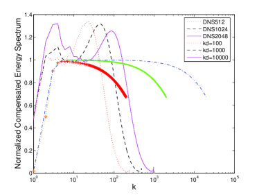
Figure 1: The normalized compensated energy spectra $\tilde{{E}}(k)=E(k)k^{5/3}/K_{Ko}$ vs. $k$ for a model energy spectrum [Eq. (8)] with $c=0.2$ and $k_{d}=100,1000,10000$, and from numerical simulations on $512^{3},1024^{3}$ and $2048^{3}$ grids at steady state. We take the energy flux $\Pi=1$ in the inertial range, so that $\tilde{{E}}(k)=1$ in the inertial range.

We compare our theoretical results with numerical simulation. The simulations have been performed for homogeneous, isotropic turbulence with stochastic forcing at low wavenumbers. These simulations were done at $512^{3}$, $1024^{3}$, and $2048^{3}$ grids. Taylor-based Reynolds numbers for these runs were approximately 240, 400 and 700 respectively. (see Yeung et al. DonzKRS:Scalar for details on simulation.) We multiply the numerical energy spectrum with $k^{5/3}/K_{Ko}$ $(K_{Ko}=1.58)$, then divide the resultant quantity by its maximum value in the inertial range, and obtain compensated energy spectrum $\tilde{{E}}(k)$. In the inertial range, $\tilde{{E}}(k)=1$. In Fig. 1 we plot $\tilde{{E}}(k)$ obtained from direct numerical simulations (DNS) done on $512^{3}$, $1024^{3}$, and $2048^{3}$ grids. A hump appears in all the DNS plots indicating the existence of the bottleneck effect in numerical simulations. These results are consistent with earlier numerical results showing the bottleneck effect.

Comparison of the normalized energy spectra for different grid resolutions reveals that the hump is most dominant for $512^{3}$, and it decreases as the grid size or Reynolds number is increased, a phenomenon observed in earlier numerical results as well Kane:Bottle ; Bran:Alpha ; Gotoh:Scalar_Bottle ; Yeung:JFM96 ; DonzKRS:Scalar . This result indicates that the bottleneck effect decreases with the increase of inertial range, thus reinforcing our hypothesis that the bottleneck effect may be due to nonavailability of sufficient range of wavenumbers to facilitate energy cascade. Please note that we have quantified the bottleneck effect by the size of the hump in the normalized energy spectrum. In individual energy spectrum the size of the hump could depend on the energy input rate etc. Also, we observe a hump at low wavenumbers which is due to the forcing at these scales. The focus of this paper is on the hump at $k\sim k_{d}$ and we will not analyze the one at the lowest waveumbers.

Let us compare the above energy spectra with a model energy spectrum for a turbulent flow Chan:RG ; Pope:book ; Pope:Hypervisc_Bottle

$$E(k)=K_{Ko}A(k/k_{f})\Pi^{2/3}k^{-5/3}\exp{(-ck/k_{d})},$$ (8)

where

$$A(x)=\frac{{x^{s+5/3}}}{1+x^{s+5/3}}$$ (9)

with forcing wavenumber $k_{f}=2$, $c=0.2$, and $s=4$. Throughout this paper we take $K_{Ko}=1.58$ Lesi:book ; McCoWatt . Clearly, $E(k)\propto k^{s}$ for $k<k_{f}$, $E(k)\propto k^{-5/3}$ for the intermediate range $(k_{f}<k<k_{d})$, and $E(k)\propto k^{-5/3}\exp(-ck/k_{d})$ for the dissipation range $(k>k_{d})$. The choice of $s=4$ is based on Batchelor’s spectra Davi:book for smaller wavenumbers. There is no hump in the model spectrum because of the choice of its functional form. Here we compare these spectra with spectra that show the bottleneck effect in order to see how the latter affects the spectral energy transport.

Without loss of generality we can take $\Pi=1$. In Fig. 1 we plot $\tilde{{E}}(k)$, which is given by

$$\tilde{{E}}(k)=E(k)k^{5/3}/K_{Ko}=A(k/k_{f})\exp{(-ck/k_{d})}$$ (10)

As expected, $\tilde{{E}}(k)$ with higher $k_{d}$ produces a larger inertial range.

In the following subsection we will compute energy flux by substituting the above energy spectra (DNS and model) in Eq. (5) and compare the results. They provide important clues for the bottleneck effect.

II.3 Bottleneck Effect in Energy Flux

First, we compute the flux $\Pi(k)$ by substituting the model energy spectrum [Eq. (8)] in Eq. (5) with $\Pi=1$. We compute the integral $I(k_{0})$ (the bracketed term of Eq. [5]) for various values of $k_{d}$. When $k_{d}=\infty$ and $A(x)=1$, the integral $I_{\infty}=0.50$ independent of $k_{0}$, implying that the flux is independent of $k_{0}$ for the Kolmogorov energy spectrum $(E(k)=K_{Ko}\Pi^{2/3}k^{-5/3})$. Using $I_{\infty}$ we find the Kolmogorov constant, $K_{Ko}=1.58$ (this is how $K_{Ko}$was computed in MKV:PR ). After this the integral $I(k_{0})$ is computed using the model spectrum with $s=4$, $c=0.2$, and $k_{d}=100,1000,10000$. The value of $I(k_{0})$ starts from 0 at $k_{0}=0$, reaches a peak, and then it decays.

The energy fluxes at various wavenumbers are

$$\Pi(k_{0})=K_{Ko}^{3/2}I(k_{0})$$ (11)

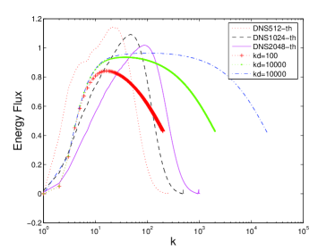
Figure 2: The computed flux $\Pi(k_{0})$ using Eq. (5) for a model energy spectrum [Eq. (8)] with $c=0.2$ and $k_{d}=100,1000,10000$, and from numerical simulations on $512^{3},1024^{3}$ and $2048^{3}$ grids at steady state.

with $K_{Ko}=1.58$. Fig. 2 contains plots of $\Pi(k_{0})$ vs. $k_{0}$ for different values of $(k_{d},c)$. The maximum values of $\Pi(k_{0})$ for these cases are listed in Table 1. They are all less than 1, but the difference from the actual value (1) is lower for larger $k_{d}$. Theoretically $max(\Pi(k_{0}))$ must be 1 because the energy input at small wavenumber is 1. The reason for the decrease in $max(\Pi(k_{0}))$ is the lack of modes in the inertial range. This is where the hump in the energy spectrum near dissipation wavenumber comes into play.

After the flux calculation for model spectrum, we compute the flux integral using $\tilde{{E}}(k)$ obtained from DNS at $512^{3}$, $1024^{3}$, and $2048^{3}$ grids, and obtain $max(\Pi_{DNS})$. These values are listed in Table 1. The value of $max(\Pi_{DNS})$ for $2048^{3}$ is very close to unity. Clearly the energy spectra obtained from numerical simulations provide a better handle on energy flux as compared to the model energy spectrum [Eq. (8)]. This is because of the higher level of energy spectrum (hump) near Kolmogorov’s wavenumber in the DNS (see Fig. 1), which makes up for the loss of large wavenumber modes. The overall effect is that the energy flux in high-resolution DNS is closer to what is expected in an idealized situation when $k_{d}\rightarrow\infty$. Thus consistency with Kolmogorov’s theory is achieved. The value $max(\Pi_{DNS})$ for $512^{3}$ is somewhat higher than 1, which may be to approximations made in our theoretical calculations.

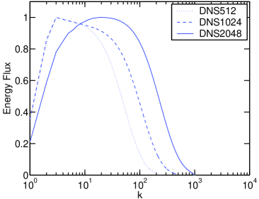
Figure 3: The normalized energy flux computed directly from DNS on $512^{3},1024^{3}$ and $2048^{3}$ grids under steady state.

The DNS plots of Fig. 2 are the fluxes computed by substituting the DNS energy spectra in Eq. (5). This exercise was done to examine the effects of the bottleneck correction in the flux. In Fig. 3 we plot the normalized energy flux computed directly from DNS data on $512^{3}$, $1024^{3}$, and $2048^{3}$ grids. The two figures match qualitatively, but not quantitatively because of the assumptions made in the field-theoretic calculation. The coupling of wavenumber modes in forced, inertial range, and dissipation range is not yet fully understood to be able to resolve $\Pi(k)$ completely from theory Alex:Imprint ; Oliv:Simulation ; Ayye ; Bras:Local .

In the present subsection we showed that the bottleneck correction near the dissipation range helps in the effective transfer of energy flux. In the next subsection we estimate the extent of the bottleneck effect to the mechanism proposed in our paper.

II.4 Estimation of the Bottleneck Effect

In this subsection we will attempt to estimate the extent of the bottleneck effect using semiquantitative arguments. Because of a lack of complete understanding of the coupling between the forced, inertial, and dissipative scales, this is the best we can do at present.

Verma et al. Ayye and Verma MKV:PR computed the shell-to-shell energy transfer rate from $m$th wavenumber shell to $n$th wavenumber shell ($T_{n}^{m}$) using

$$T_{n}^{m}=K_{Ko}^{3/2}\Pi\left[\int_{k\in s_{n}}dkk{}^{2}\int_{p\in s_{m}}dp\int_{|k-p|}^{k+p}dq\frac{{pq}}{4k}\frac{{T_{1}C(p)C(q)+T_{2}C(q)C(k)+T_{3}C(p)C(k)}}{\nu^{*}(k^{2/3}+p^{2/3}+q^{2/3})}\right],$$ (12)

where $s_{m,n}$ are the wavenumber range for the $m$th and $n$th shell respectively. The wavenumber space is divided into various shells logarithmically. In Verma et al. Ayye and Verma MKV:PR the $m$th shell is $(2^{m/4}:2^{(m+1)/4})$.

Verma et al. Ayye and Verma MKV:PR computed $T_{n}^{m}$ in the inertial range using a similar procedure as described in the previous subsection. Kolmogorov’s spectrum $k^{-5/3}$ was assumed through out the wavenumber space. They found that the energy transfer is maximal to the nearest neighbour, yet significant energy is transferred to other shells. For example, the energy transfer rates from $m$th shell the shells $m+1$, $m+2$, and $m+3$ are 18%, 6.7%, and 3.6% respectively. The transfer rate decreases monotonically for more distant shells.

Let us imagine a wavenumber sphere of radius $R$ somewhat in the middle of the inertial range. Using the shell-to-shell energy transfer rates we can compute the energy transfers from the above wavenumber sphere to $n$ shells adjacent to the sphere (wavenumber range $[R:R*2^{n/4}])$. Simple algebra shows that the above quantity is MKV:PR

$$\frac{{Q_{n}}}{\Pi}=\sum_{m=1}^{n}m\times T_{n}^{m}.$$ (13)

In Table 2 we list $Q_{n}$ for various values of $n$. The Table shows that 42.2% of the flux is transferred to the three adjacent shells. To transfer 99.1% energy we need 28 shells in the right of the sphere. Therefore, we require large number of wavenumber shells for effective energy transfer, and the bottleneck effect is expected if the inertial range is insufficient. In this theory, the bottleneck effect would disappear when there are sufficient wavenumber shells to enable the complete energy transfer.

The energy transfer among the wavenumber shells is antisymmetric, that is $T_{n}^{m}=-T_{m}^{n}$. If we assume the above mentioned waveumber sphere to be in the middle of the inertial range, we require approximately $28\times 2=56$ shells for an effective energy transfer. Hence, the inertial range $(k_{max}/k_{min})$ required must be around $2^{56/4}\approx 10^{4}$. Hence our estimate for the minimum length of the inertial range for no bottleneck effect is approximately four decades. The range of inertial range in all the experiments and simulations discussed in this paper is less than four decades, and the bottleneck effect is observed in all of them. Hence our theoretical estimate is consistent with the present experimental and numerical results. We remark that the above estimate of the required inertial range for zero bottleneck effect could be an overestimate. A realistic estimate requires a detailed study of energy transfer among modes in the whole range: forcing, inertial, and dissipation range.

After the above estimation of required inertial range to suppress the bottleneck, we move on to estimate the increase in the energy spectrum due to the bottleneck effect. Suppose the energy spectrum $E(k)$ till the dissipation wavenumber is

$$E(k)=K_{Ko}\Pi^{2/3}k^{-5/3}(1+e(k)),$$ (14)

where $e(k)=\delta E(k)/E(k)$ is the normalized bottleneck correction. There is a complex interaction between the wavenumbers in the forcing, inertial, and dissipation range, which is not yet completely understood. For time being we estimate the additional energy transfer due to the bottleneck correction to be of the order of $T_{bottleneck}\sim\Pi\times e(k_{d})$. Since the energy supplied at the large-scales has to reach the dissipation scale, and if the number of wavenumber shells to the right of above mentioned wavenumber sphere is $n$, then

$$\frac{{Q_{n}}}{\Pi}+\frac{{T_{bottleneck}}}{\Pi}\approx 1.$$ (15)

Therefore,

$$e(k_{d})=\frac{{\delta E(k_{d})}}{E_{Kolm}(k_{d})}\approx\left[1-\frac{{Q_{n}}}{\Pi}\right].$$ (16)

Using Zhou Zhou:Local and Verma et al.’s results Ayye that $T_{n}^{m}\approx|n-m|^{-4/3}$ for small $(n-m)$, we estimate

$$\frac{{Q_{n}}}{\Pi}\approx\alpha n^{2/3}$$ (17)

where $\alpha$ is a positive constant. Assuming that the we have equal number of wavenumber shells to the left and right of the wavenumber sphere $R$ discussed above, the ratio of Kolmogorov’s wavenumber and forcing wavenumbers is approximately

$$\frac{{k_{d}}}{k_{0}}\sim Re^{3/4}\sim(2^{n/4}\times 2^{n/4}),$$ (18)

which yields $n\sim 1.5\log_{2}Re$, where $Re$ is the Reynolds number based on Kolmogorov’s scale. Substituting this estimate of $n$ in Eq. (16) we obtain

$$e(k_{d})\sim 1-\alpha(1.5\log_{2}Re)^{2/3},$$ (19)

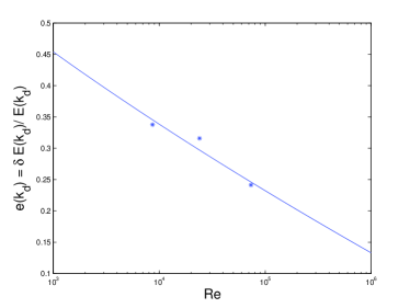
Figure 4: A plot of our estimated normalized bottleneck correction $e(k_{d})=\delta E(k_{d})/E(k_{d})$ [Eq. (19)] as a function of Reynold number $Re$. The three points ($*$) represent $[Re,e(k_{d})]$ for DNS on $512^{3},1024^{3}$ and $2048^{3}$ grids at steady state.

which is plotted in Fig. 4 for a reference with $\alpha=0.09$. The three points represent the $(Re,e(k_{d}))$ for three DNS discussed in the present paper. The choice of $\alpha=0.09$ fits best with the DNS values, and it is consistent with our $Q_{n}$equation [Eq. (17)]. The numerical values of DNS fit quite well with the theoretical predictions, however, we need more DNS results for a better test of our theoretical estimate of the bottleneck correction. Also, for $\alpha=0.09$, $e(k_{d})\approx 0$ for $n\approx 37$ and $Re\approx 10^{7}$. These estimates are in reasonable agreement with our earlier estimate of the length of the inertial range for zero bottleneck effect. Our prediction of $e(k_{d})$ is proportional to $1-\mbox{const}(\log Re)^{2/3}$, and it differs from the predictions of earlier theories.

Please note that the above expression for $e(k_{d})$ is only a crude approximation, and could be an overestimate. To better understand the bottleneck effect we need to understand the coupling among forcing, inertial, and dissipation scales, as well as other aspects like intermittency.

The dynamics at the dissipation rate is quite important in the study of the bottleneck effect. This is evident from the numerical observations of Lamorgese et al. Pope:Hypervisc_Bottle , Biskamp et al. Bisk:Bottle_2D , and Dobler et al. Bran:Bottle who reported that hyperviscosity enhances the bottleneck effect. Since the extent of inertial range increases with the introduction of hyperviscosity, it may appear that the bottleneck effect should decrease in the presence of hyperviscosity. However, that is not the case. This result is possibly because of the shorter dissipation range in the presence of hyperviscosity, and the hump in the energy spectrum near $k_{d}$ could help in the inertial-range energy transfer as well as in the dissipation of energy. This is an important question to investigate. So far our focus has been on the physics of energy transfer in the inertial range. A more detailed study of energy exchange between wavenumbers in the inertial and dissipative range is required for a conclusive statement Alex:Imprint ; Bras:Local .

III Conclusions

To summarize, in this paper we investigated the reason for the bottleneck effect in turbulence. The energy is supplied at large scales, and it cascades to smaller scales. Recent numerical and theoretical studies show that even though most of the energy from a given wavenumber shell goes to the next wavenumber shell, there is a significant energy transfer to the distant wavenumber shells. We showed that an effective transfer of energy flux in the inertial range can take place when there is approximately four decades of inertial range. If the inertial range is shorter, a hump is created near Kolmogorov’s scale (beginning of dissipation range) which compensates for the nonexistence of required inertial range. The bottleneck effect is observed in most of the current numerical simulations and experiments.

The mechanism proposed in the present paper differs from that of Falkovich Falk:Bottleneck and Yakhot and Zakharov YakhZakh:Cleb . Falkovich Falk:Bottleneck argued that the bottleneck effect is due to the suppression of nonlinear interactions by dissipative modes, and it is present for all dissipative turbulence systems. Falkovich assumes essentially a local energy cascade in contrast to both local and nonlocal transfers in our mechanism. In our picture, the energy is transferred to the dissipative scales not only from its immediate neighbouring wavenumber shells, but also from the middle of inertial range. The energy transfer by Kolmogorov’s spectrum requires certain minimum inertial range. If this range is not present, the energy levels of the modes near Kolmogorov’s scales increase to facilitate the energy transfer. Note that if full range of inertial range is present, the last wavenumber shells in the inertial range would transfer only a small fraction of energy flux, and there is no bottleneck effect. Our theory suggests that the bottleneck effect will disappear if the inertial range is more than approximately four decades. Yakhot and Zakharov YakhZakh:Cleb and She and Jackson She:Bottle obtained $k^{-1}$ bottleneck correction. Our model purely based on energy flux differs from these theories as well. Quantitatively, our prediction for the bottleneck correction $e(k_{d})$ is proportional to $1-\mbox{const}(\log Re)^{2/3}$, and it differs from the predictions of earlier theories.

Traditional shell models of turbulence assume local energy transfers, and have a large inertial range ($2^{15-20}\sim 10^{5-10}$). The bottleneck effect is generally not observed in the shell models. However Biferale and kerr Bife:ShellBottle report the bottleneck effect in a shell-model ($n=15$) based on Kerr-siggia model. So shell models with small inertial range could show bottleneck effect, but the bottleneck effect in shell model is in the spirit of Falkovich’s mechanism; there is not enough dissipative scale to dissipate the cascaded energy.

The “real” turbulence however involves local as well as nonlocal energy transfers that are not simulated in local shell models of turbulence. The recent nonlocal shell models Step:NonlocalShell attempt to model these features of turbulence, and it will be interesting to investigate bottleneck effect in the nonlocal shell models. We remark that the field-theoretic calculation presented in this paper is more fundamental than the shell model, and some of it’s features are same as the shell model. Still it is instructive to independently investigate bottleneck effect using nonlocal shell model.

Many important and unresolved issues are involved in the study of the bottleneck effect. We need to fully understand the nonlinear coupling between the forcing, inertial, and dissipative range (see Alexakis et al. Alex:Imprint , Debliquy et al. Oliv:Simulation , Verma et al. Ayye , Brasseur and Wei Bras:Local for some of the recent attempts). The vortex interactions, intermittency etc. also come up in the study of the bottleneck effect, and we need to understand them better as well.

The energy transfer in the turbulence of passive scalar and magnetohydrodynamics follows similar patterns as in fluid turbulence. The energy transfer is forward and local, yet significant range of inertial-range is required for effective energy transfer Ayye:MHD . Hence we expect the bottleneck effect to be present in these systems as well. These projections are consistent with a strong bottleneck effect observed in numerical simulations of Watanabe and Gotoh Gotoh:Scalar_Bottle and Yeung et al. DonzKRS:Scalar ; Yeung:JFM96 for passive-scalar turbulence, and those of Haugen et al. Bran:Flux for MHD turbulence. The bottleneck effect has been observed in electron-magnetohydrodynamic (EMHD) turbulence, and two-dimensional turbulence (see Biskamp et al. Bisk:Bottle_2D and references therein), but its cause is possibly more complex. It has been observed that the bottleneck effect along the transverse and longitudinal directions are different Veer:Bottle ; this result still lacks satisfactory explanation. Future developments in theoretical turbulence will possibly resolve some of these issues.

Table 1: The maximum values of energy fluxes for the model energy spectra [Eq. (8)] with $c=0.2$ and $k_{d}=100,1000,10000$, and for energy spectra obtained from numerical simulations on $512^{3},1024^{3}$ and $2048^{3}$ grids. For Kolmogorov’s spectrum $max(\Pi(k_{0}))=1$.

	$k_{d}$	$max(\Pi(k_{0}))$
kd100	100	0.84
kd1000	1000	0.94
kd10000	10000	0.96
DNS512	-	1.14
DNS1024	-	1.09
DNS2048	-	1.02

Table 2: The energy transfer rates from a wavenumber sphere in the inertial range to $n$ shells adjacent to the sphere $(Q_{n}/\Pi=\sum_{m=1}^{n}m*T_{n}^{m})$ for various $n$’s.

$n$	1	2	3	8	13	28	32	48
$2^{n/4}$	$2^{1/4}$	$2^{1/2}$	$2^{3/4}$	4	95	128	256	4098
$Q_{n}/\Pi$	0.18	0.32	0.42	0.74	0.88	0.99	0.99	$\sim 1$

Figures