Abstract

Nonlinear contraction theory is a comparatively recent dynamic control system design tool based on an exact differential analysis of convergence, in essence converting a nonlinear stability problem into a linear time-varying stability problem. Contraction analysis relies on finding a suitable metric to study a generally nonlinear and time-varying system. This paper shows that the computation of the metric may be largely simplified or indeed avoided altogether by extending the exact differential analysis to the higher-order dynamics of the nonlinear system. Simple applications in economics, classical mechanics, and process control are described.

1 Introduction

Nonlinear contraction theory is a comparatively recent dynamic control system design tool based on an exact differential analysis of convergence [12]. In essence, it allows one to convert a nonlinear stability problem into a linear time-varying stability problem. Contraction analysis relies on finding a suitable metric to study a generally nonlinear and time-varying system. Depending on the application, the metric may be trivial (identity or rescaling of states), or obtained from physics, combination of contracting subsystems [12], semi-definite programming [13], or recently sums-of-squares programming [2].

The goal of this paper is to show that the computation of the metric may be largely simplified or avoided altogether by extending the exact differential analysis to the higher-order dynamics of the nonlinear system. Intuitively this is not surprising, since, as an elementary instance, a scalar linear time-invariant system would require in the original approach a non-identity metric (obtained from a Lyapunov Matrix Equation).

After a brief review of contraction theory in Section 2, the main results are presented in Section 3, first in the discrete-time case (with a simple application to price dynamics in economics) and then in the continuous-time case. Simple examples and applications are discussed in Section 4, in the contexts of classical mechanics, process control, and observer design (see [1, 17, 9, 20] for other recent applications of contraction theory to observer design). Hamiltonian systems are studied in section 5. Concluding remarks are offered in section 6.

2 Contraction theory

The basic theorem of contraction analysis [12] can be stated as

Theorem 1

Consider the deterministic system $\ \dot{\bf x}={\bf f}({\bf x},t)\$, where ${\bf f}$ is a smooth nonlinear function. If there exist a uniformly positive definite metric

${\bf M(\bf x},t)\ =\ {\bf\Theta}({\bf x},t)^{T}\ {\bf\Theta}^{\ast}({\bf x},t)$

such that the Hermitian part of the associated generalized Jacobian ${\bf F}\ =\ \left(\dot{\bf\Theta}+{\bf\Theta}\frac{\partial{\bf f}}{\partial{\bf\bf x}}\right){\bf\Theta}^{-\ast}$

is uniformly negative definite, then all system trajectories converge exponentially to a single trajectory, with convergence rate $|\lambda_{max}|$, where $\lambda_{max}$ is the largest eigenvalue of the Hermitian part of $\ {\bf F}$. The system is said to be contracting.

In the above, $\ {}^{\ast}$ denotes complex conjugation, $\ {}^{-\ast}$ for a matrix denotes the inverse of the conjugate matrix, and the state-space is $R^{n}$ (in this paper) or $C^{n}$. The system is said to be semi-contracting (for the metric ${\bf M(\bf x},t)$) if ${\bf F}$ is always negative semi-definite, and indifferent if ${\bf F}$ is always zero.

It can be shown conversely that the existence of a uniformly positive definite metric with respect to which the system is contracting is also a necessary condition for global exponential convergence of trajectories. In the linear time-invariant case, a system is globally contracting if and only if it is strictly stable, with ${\bf F}$ simply being a normal Jordan form of the system and ${\bf\Theta}$ the coordinate transformation to that form. Conceptually, approaches closely related to contraction, although not based on differential analysis, can be traced back to [8] and even to [11].

Similarly, a discrete system

$${\bf x}_{i+1}={\bf f}_{i}({\bf x}_{i},i)$$

will be contracting in a metric ${\bf\Theta}^{T}{\bf\Theta}^{\ast}$ if the largest singular value of the discrete Jacobian ${\bf\Theta}_{i+1}\frac{\partial{\bf f}_{i}}{\partial{\bf x}_{i}}{\bf\Theta}_{i}^{-\ast}$ is strictly smaller than 1. In the particular case of real autonomous systems with identity metric, the basic contraction theorem corresponds in the continuous-time case to Krasovkii’s theorem [19], and in the discrete-time case to the contraction mapping theorem [3].

Contraction theory proofs make extensive use of virtual displacements, which are differential displacements at fixed time borrowed from mathematical physics and optimization theory. Formally, if we view the position of the system at time $t$ as a smooth function of the initial condition ${\bf x}_{o}$ and of time, $\ {\bf x}={\bf x}({\bf x}_{o},t)\$, then $\ \delta{\bf x}=\frac{\partial{\bf x}}{\partial{\bf x}_{o}}\ d{{\bf x}_{o}}\$. For instance [12], for the system of Theorem 1, one easily computes

$$\frac{d}{dt}({\bf\Theta}\delta{\bf x})\ =\ {\bf F}({\bf\Theta}\delta{\bf x})$$ (1)

An appropriate metric to show that the system is contracting may be obtained from physics, combination of contracting subsystems [12], semi-definite programming [13], or sums-of-squares programming [2]. The goal of this paper is to show that the computation of the metric may be largely simplified or avoided altogether by considering the system’s higher-order virtual dynamics (rather than merely its first-order virtual dynamics, as in equation (1)).

3 Higher-order contraction

3.1 The discrete-time case

Technically, the extension to higher-order contraction is simplest in the discrete-time case, which we discuss first. The main idea is to construct an exponential bound on the virtual displacement $\delta{\bf x}$ over $n$ time-steps, rather than over a single time-step as in [12].

Consider for $i\geq 0$ the $n$-dimensional ($n\geq 1$) virtual dynamics

$$\delta{\bf x}_{i+n}={\bf A}^{n-1}_{i}\delta{\bf x}_{i+n-1}+\ldots+{\bf A}^{o}_{i}\delta{\bf x}_{i}$$

Taking the norm (denoted by $|\ \ |$ ) on both sides, and bounding, yields

$$|\delta{\bf x}_{i+n}|\ \leq\ \ |A^{n-1}_{i}|\ |\delta{\bf x}_{i+n-1}|\ +\ \ldots\ +\ |A^{o}_{i}|\ |\delta{\bf x}_{i}|$$

where the norm of a matrix is the largest singular value of that matrix. Let us bound for $i=0$ the initial conditions using real positive constants $\lambda$ and $K$ as

$$|\delta{\bf x}_{j}|\leq K\lambda^{j},\ 0\leq j<n$$

Assume now that the following characteristic equation is verified,

$$\lambda^{n}\geq|A^{n-1}_{i}|\lambda^{n-1}+\ldots+|A^{o}_{i}|,\ \forall i\geq 0$$

We then get

$$|\delta{\bf x}_{i+n}|\leq|A^{n-1}_{i}|K\lambda^{i+n-1}+\ldots+|A^{o}_{i}|K\lambda^{i}\leq K\lambda^{i+n}$$

Figure 1: $\pm K\lambda^{i}$ defined by $\delta x_{i}$ over $i$

Repeating the above recursively for $i\geq 0$ we get by complete induction

$$|\delta{\bf x}_{i}|\leq K\lambda^{i}$$

and hence exponential convergence of $|\delta{\bf x}_{i}|$, as illustrated in Figure 3.

Theorem 2

Consider for $i\geq 0$ the $n$-dimensional ($n\geq 1$) virtual dynamics

$$\delta{\bf x}_{i+n}={\bf A}^{n-1}_{i}\delta{\bf x}_{i+n-1}+\ldots+{\bf A}^{o}_{i}\delta{\bf x}_{i}$$

Let us define $\forall i\geq 0$ a constant $\lambda$ with the characteristic equation

$$\lambda^{n} \geq |A^{n-1}_{i}|\lambda^{n-1}+\ldots+|A^{o}_{i}|,\ \forall i\geq 0\$$ (2)

We can then conclude

$$|\delta{\bf x}_{i+n}|\leq K\lambda^{i+n}$$

where $K$ is defined by

$$|\delta{\bf x}_{j}|\leq K\lambda^{j},\ 0\leq j<n\$$ (3)

Thus, the system is contracting if $\ \lambda<1$.

• Example 3.1

  : Consider first a second-order linear time invariant (LTI) dynamics

  $$x_{i+2}\ +\ 2\ \gamma\ x_{i+1}\ +\ \alpha\gamma^{2}x_{i}\ =\ u_{i}$$

  where $u_{i}$ is an input, and $\gamma$ and $\alpha$ are constants. The virtual dynamics is

  $$\delta x_{i+2}=-\ 2\ \gamma\ \delta x_{i+1}\ -\ \alpha\gamma^{2}\ \delta x_{i}$$

  The characteristic equation (2) for $\lambda\geq 0$ is then given by

  $$\lambda^{2}\ \geq\ 2\ |\gamma|\ \lambda+|\alpha|\gamma^{2}\ \ \ \ \ \ \ \ \ i.e.\ \ \ \ \ \ \ \ \ \lambda\ \geq\ |\gamma|(1+\sqrt{1+|\alpha|\ })$$

  Thus, the contraction condition $\lambda<1$, or

  $$|\gamma|(1+\sqrt{1+|\alpha|\ })\ <\ 1$$

  simply means that both eigenvalues of the system have to lie for the conjugate complex case ($\alpha>1$) within the red half circles in (2) or on the green line for the real case ($\alpha\leq 1$). Note that Theorem 2 simply bounds the possibly oscillating discrete system with a non-oscillating system of the same convergence rate for the real case.

  Consider now the virtual dynamics of an arbitrary second-order nonlinear time-varying system,

  $$\delta x_{i+2}+\ 2\ \gamma(i)\ \delta x_{i+1}+\alpha(i)\ \gamma^{2}(i)\delta x_{i}\ =\ 0$$

  The characteristic equation and the contraction condition are the same as above, except that $\ \gamma\$ and $\ \alpha\$ are now time-dependent.

  

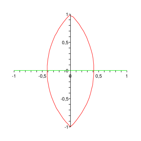
  Figure 2: Contraction region in the complex plane of second-order discrete system

  $\Box$

• Example 3.2

  : In economics, consider the price dynamics

  $${\bf n}_{i+1} = {\bf f}_{i}({\bf p}_{i},i)$$

  $${\bf p}_{i+1} = {\bf g}_{i}({\bf n}_{i},i)$$

  with ${\bf n}_{i}$ the number of sold products at time $i$ and corresponding price ${\bf p}_{i}$.

  The first line above defines the customer demand as a reaction to a given price. The second line defines the price, given by the production cost under competition, as a reaction to the number of sold items. The dynamics above corresponds to the second-order economic growth cycle dynamics

  $${\bf n}_{i+2}={\bf f}_{i+1}\left({\bf g}_{i}({\bf n}_{i},i)\right)$$

  Contraction behavior of this economic behavior with contraction rate $\lambda$ can then be concluded with Theorem 2 for

  $$\lambda^{2}\geq|\frac{\partial{\bf f}_{i+1}}{\partial{\bf p}_{i+1}}\frac{\partial{\bf g}_{i}}{\partial{\bf n}_{i}}|$$ (4)

  That means we get stable (contraction) behavior if the product of customer demand sensitivity to price and production cost sensitivity to number of sold items has singular values less than 1. We can get unstable (diverging) behavior for the opposite case.

  Note that this result even holds when no precise model of the sensitivity is known, which is usually the case in economic or game situations.

  Whereas the above is well known for LTI economic models we can see that the economic behavior is unchanged for a non-linear, time-varying economic environment.

  Let as assume now that the above corresponds to a game situation (see e.g. [18] or [5]) between two players with strategic action ${\bf p}_{i}$ and ${\bf n}_{i}$. Both players optimize their reaction ${\bf g}$ and ${\bf f}$ with respect to the opponent’s action.

  We can then again conclude for (4) to global contraction behavior to a unique time-dependent trajectory (in the autonomous case, the Nash equilibrium). $\Box$

Of course, and throughout this paper, in some cases the analysis may yet be further streamlined by first applying a simplifying metric transformation of the form $\ \delta{\bf z}={\bf\Theta}\delta{\bf x}\$, and then applying the results to $\ \delta{\bf z}$.

3.2 The continuous-time case

Let us now derive the continuous-time version of the previous results. Consider for $t\geq 0$ the $n$-dimensional ($n\geq 1$) virtual dynamics

$$\delta{\bf x}^{(n)}=-{\bf A}_{n-1}\delta{\bf x}^{(n-1)}-\ ...\ -{\bf A}_{o}\delta{\bf x}$$

The proof is based on splitting up the dynamics into a stable part, described by a block diagonal matrix composed of identical negative definite blocks ${\bf F}$ which we select, and an unstable higher-order part. Let $\delta{\bf x}_{o}=\delta{\bf x}$, and define recursively

$$\delta\dot{\bf x}_{o} = {\bf F}\delta{\bf x}_{o}+\delta{\bf x}_{1}$$

$$...$$

$$\delta\dot{\bf x}_{n-2} = {\bf F}\delta{\bf x}_{n-2}+\delta{\bf x}_{n-1}$$

$$\delta\dot{\bf x}_{n-1} = -{\bf A}_{n-1}\delta{\bf x}_{o}^{(n-1)}-{\bf A}_{n-2}\delta{\bf x}_{o}^{(n-2)}-\ ...\ -{\bf A}_{o}\delta{\bf x}_{o}$$ (5)

$$-\left({\bf F}\delta{\bf x}_{o}\right)^{(n-1)}-...-\left({\bf F}\delta{\bf x}_{n-2}\right)^{(1)}$$

$$= -{\bf A}_{n-1}\left({\bf F}\delta{\bf x}_{o}+\delta{\bf x}_{1}\right)^{(n-2)}-...-{\bf A}_{o}\delta{\bf x}_{o}$$

$$-\left(L^{1}{\bf F}\delta{\bf x}_{o}+L^{o}{\bf F}\delta{\bf x}_{1}\right)^{(n-2)}-...-\left(L^{1}{\bf F}\delta{\bf x}_{n-2}+L^{o}{\bf F}\delta{\bf x}_{n-1}\right)$$

$$= {\bf F}\delta{\bf x}_{n-1}-{\bf A}_{n-1}^{\ast}\delta{\bf x}_{n-1}-{\bf A}_{n-2}^{\ast}\delta{\bf x}_{n-2}-{\bf A}_{n-3}^{\ast}\delta{\bf x}_{n-3}-...$$

where

$$L^{o}{\bf F} = {\bf F}$$

$$L^{j}{\bf F} = \frac{d}{dt}L^{j-1}{\bf F}+L^{j-1}{\bf F}\ {\bf F}\ \ \ \ \ \ \ \ \ j\geq 1$$

and

$${\bf A}_{n-1}^{\ast} = {\bf A}_{n-1}+\left(\begin{array}[]{c}n\\ 1\end{array}\right)L^{o}{\bf F}$$ (8)

$${\bf A}_{n-2}^{\ast} = {\bf A}_{n-2}+\left(\begin{array}[]{c}n-1\\ 1\end{array}\right){\bf A}_{n-1}L^{o}{\bf F}+\left(\begin{array}[]{c}n\\ 2\end{array}\right)L^{1}{\bf F}$$ (13)

$${\bf A}_{n-3}^{\ast} = {\bf A}_{n-3}+\left(\begin{array}[]{c}n-2\\ 1\end{array}\right){\bf A}^{n-2}L^{o}{\bf F}+\left(\begin{array}[]{c}n-1\\ 2\end{array}\right){\bf A}^{n-1}L^{1}{\bf F}+\left(\begin{array}[]{c}n\\ 3\end{array}\right)L^{2}{\bf F}$$

$$...$$

Equation (5) represents the superposition of a higher-order-system and a block diagonal dynamics in the chosen ${\bf F}$. Let us assess the contraction behavior of the higher-order part by taking the norm

$$|\delta{\bf x}^{(n)}|\leq|{\bf A}_{n-1}^{\ast}||\delta{\bf x}^{(n-1)}|+|{\bf A}_{n-2}^{\ast}||\delta{\bf x}^{(n-2)}|+\ \ldots\$$

where the norm of a matrix is the largest singular value of that matrix. Let us bound for $t=0$ the initial conditions with real and constant $\lambda,K\geq 0$ and assume the following characteristic equation

$$|\delta{\bf x}^{(j)}| \leq K\lambda^{j}e^{\lambda t},\ \ \ \ \ \ \ \ \ \ \ \ \ \ \ \ \ \ \ \ \ \ \ 0\leq j<n\$$ (21)

$$\lambda^{n} \geq |{\bf A}_{n-1}^{\ast}|\lambda^{n-1}+\ \ldots\ +|{\bf A}_{o}^{\ast}|,\ \forall t\geq 0$$ (22)

Figure 3 shows how $K$ has to be selected for a given $\lambda$ for a second-order system ($n=2$).

Figure 3: $Ke^{\lambda t}$ bounding the first and second derivative of $\delta x$ for a given $\lambda$ at $t=0$

With (22) we can bound the $n$’th derivative of $\delta{\bf x}$ as

$$|\delta{\bf x}^{(n)}|\leq|{\bf A}_{n-1}^{\ast}|K\lambda^{n-1}e^{\lambda t}+\ \ldots\ +|{\bf A}_{o}^{\ast}|Ke^{\lambda t}\leq K\lambda^{n}e^{\lambda t}$$

Integrating the above for $t\geq 0$ we can exponentially bound the higher-order dynamics $\delta{\bf x}$ as

$$|\delta{\bf x}|\leq Ke^{\int_{o}^{t}\lambda d\tau}$$

Using the above this allow to conclude:

Theorem 3

Consider for $t\geq 0$ the $n$-dimensional ($n\geq 1$) virtual dynamics

$$\delta{\bf x}^{(n)}=-{\bf A}^{n-1}\delta{\bf x}^{(n-1)}-\ \ldots\ -{\bf A}^{o}\delta{\bf x}$$

Let us define a constant $\lambda\geq 0$ such that $\forall t\geq 0$ we fulfill the characteristic equation

$$\lambda^{n}\geq{\bf A}_{n-1}^{\ast}\lambda^{n-1}+\ \ldots\ +{\bf A}_{o}^{\ast}$$ (23)

where ${\bf A}_{j}^{\ast}$ is defined in (8) for a given choice of the matrix ${\bf F}$.

We can then conclude on contraction rate (i.e., the largest eigenvalue of the symmetric part of) ${\bf F}+\lambda{\bf I}$, where $|\delta{\bf x}|$ is initially bounded with $K$, defined in (21).

One specific choice of ${\bf F}$ is $-\frac{{\bf A}_{n-1}}{n}$, which cancels the highest time-derivative on the right-hand side, and is known for LTV systems as the reduced or unstable form [10] of the original higher-order dynamics. We will use this definition of ${\bf F}$ in most of the following examples. Also note that more general forms could be chosen for the stable part.

4 Examples and Applications

In this section, we discuss simple examples (section 4.1), applications to nonlinear observer design (section 4.2), and adding an indifferent system (section 4.3).

4.1 Some simple examples

• Example 4.1

  : Consider the second-order LTI dynamics

  $$\ddot{x}=-2\zeta\omega\dot{x}-\omega^{2}x$$

  with constant $\zeta$ and $\omega\geq 0$. The virtual dynamics is

  $$\delta\ddot{x}=-2\zeta\omega\delta\dot{x}-\omega^{2}\delta x$$

  The characteristic equation (23) is then given with $F=\zeta\omega$ for constant, positive $\lambda$ by

  $$\lambda^{2}\geq|-\omega^{2}+\frac{(2\zeta\omega)^{2}}{4}|=|\zeta^{2}-1|\omega^{2}\ \ \ \ \ \ \ \ \ \rm{i.e.}\ \ \ \ \ \ \ \ \ \lambda\geq\omega\sqrt{|\zeta^{2}-1|}$$

  Using Theorem 3 we can then conclude on contraction behavior with convergence rate

  $$\omega(-\zeta+\sqrt{|\zeta^{2}-1|})$$

  This means that we require the poles to lie within the $\pm 45^{o}$ quadrant of the left-half complex plane. $\Box$

While Theorem 3 can thus be overly conservative for LTI systems, this is not the case for general nonlinear time-varying systems, as we now illustrate.

• Example 4.2

  : Consider the second-order LTV dynamics

  $$\ddot{x}+a_{1}\ \dot{x}+a_{o}(t)\ \ x=u(t)$$

  with $a_{1},a_{o}\geq 0$, which would be sufficient conditions for LTI stability. Let us assume a small damping gain $a_{1}$ and strong spring gains $a_{o}$ such that the system oscillates.

  If now the time-varying gain $a_{o}(t)$ is chosen to be very large when the system oscillates back to $0$ and small otherwise then the energy is constantly increased, which makes the system unstable (Figure 4). This is precisely what is excluded by Theorem 3. $\Box$

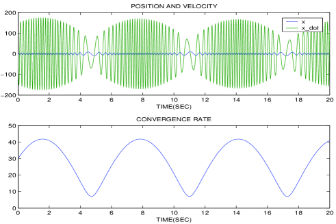
Figure 4: LTV system with $a_{0}=900+850\sin t$ and $a_{1}=0.01$

• Example 4.3

  : Consider the second-order LTV dynamics

  $$\ddot{x}+a_{1}(t)\ \dot{x}+a_{o}(t)\ x=u(t)$$

  The virtual dynamics is

  $$\delta\ddot{x}=-a_{1}\delta\dot{x}-a_{o}\delta x$$

  The characteristic equation (23) is then given with $F=-\frac{a_{1}}{2}$ by

  $$\lambda^{2}\geq|-a_{o}+\frac{a_{1}^{2}}{4}+\frac{\dot{a_{1}}}{2}|$$

  for constant positive $\lambda$. Using Theorem 3 we can then conclude on contraction behavior with convergence rate $-\frac{a_{1}}{2}+\lambda\$ (Figure 5). $\Box$

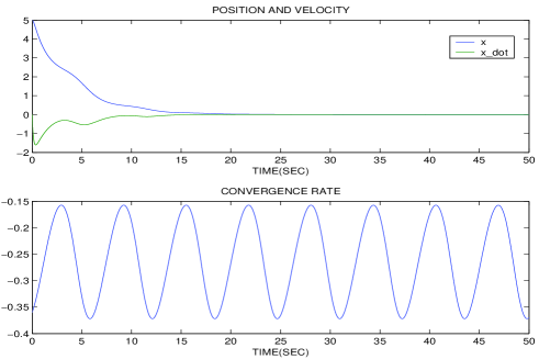
Figure 5: LTV system with $a_{0}=2+\cos t$ and $a_{1}=8+\sin t$

• Example 4.4

  : Let us illustrate a case where choosing ${\bf F}$ other than $\ -\frac{{\bf A}_{n-1}}{n}\$ can simplify the result. Consider the generalized Van der Pol or Lienard dynamics

  $$\ddot{x}=-a_{1}(x)\dot{x}-a_{o}(x,t)$$

  with $a_{1},\frac{\partial a_{o}}{\partial x}\geq 0$. The virtual dynamics is

  $$\delta\ddot{x}=-a_{1}\delta\dot{x}-\left(\frac{\partial a_{o}}{\partial x}+\dot{a_{1}}\right)\delta x$$

  The characteristic equation (23) is then given with $F=-a_{1}+\frac{\min(a_{1})}{2}$ by

  $$\lambda^{2}=(a_{1}-\min(a_{1}))\lambda+|-\frac{\min(a_{1})^{2}}{4}+\frac{a_{1}\min(a_{1})}{2}-\frac{\partial a_{o}}{\partial x}|$$

  and hence $\lambda\geq 0.5\left(a_{1}-\min(a_{1})+\sqrt{(a_{1}-\min(a_{1}))^{2}+|-\min(a_{1})^{2}+2a_{1}\min(a_{1})-4\frac{\partial a_{o}}{\partial x}|}\right)$. Thus the contraction behavior of $\delta x$ is then given by

  $$\lambda+F\leq-0.5a_{1}+0.5\sqrt{(a_{1}-\min(a_{1}))^{2}+|-(a_{1}-\min(a_{1}))^{2}+a_{1}^{2}-4\frac{\partial a_{o}}{\partial x}|}$$

  which is negative if the argument of the square root is less than $a_{1}^{2}$, i.e. for $\min(a_{1})^{2}-2a_{1}\min(a_{1})+4\frac{\partial a_{o}}{\partial x}\leq 0$.

  Hence we can conclude on contraction behavior if the poles of the minimal damping $\min(a_{1})$ with the actual spring gain $\frac{\partial a_{o}}{\partial x}$ lie within the $\pm 45^{o}$ quadrant of the left-half complex plane (Figure 6). Note that this result can be extended to the vector case ${\bf x}$ if the corresponding matrix $A_{1}({\bf x})$ is integrable. $\Box$

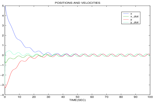
Figure 6: Van der Pol with $a_{1}=8+\sin x$ and $u(t)=\cos t$

• Example 4.5

  : Consider the second-order nonlinear vector system

  $$\ddot{\bf x}+{\bf D}\ \dot{\bf x}+\frac{\partial V}{\partial{\bf x}}=u(t)$$

  with potential energy $V=x_{1}^{2}+x_{2}^{2}+x_{1}x_{2}\sin t$ and constant damping gain ${\bf D}=diag(1,4)$.

  The corresponding variational dynamics is

  $$\delta\ddot{\bf x}+{\bf D}\ \delta\dot{\bf x}+\frac{\partial^{2}V}{\partial{\bf x}^{2}}\ \delta{\bf x}=0$$

  The characteristic equation (23) for ${\bf F}=-\frac{\bf D}{2}$ is then given by

  $$\lambda^{2}\geq|\frac{\partial^{2}V}{\partial{\bf x}^{2}}-\frac{\bf DD}{4}\ |$$

  for constant positive $\lambda$. Using Theorem 3 we can then conclude on contraction behavior with convergence rate $\ \lambda{\bf I}\ -\frac{\bf D}{2}$ in Figure 7. $\Box$

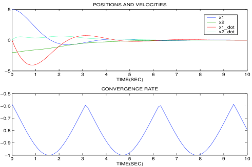
Figure 7: Second-order system with ${\bf D}=diag(1,4)$ and $V=x_{1}^{2}+x_{2}^{2}+x_{1}x_{2}\sin t$

• Example 4.6

  : Let us consider two coupled systems of the same dimensions, with the virtual dynamics

  $$\frac{d}{dt}\left(\begin{array}[]{c}\delta{\bf x}_{1}\\ \delta{\bf x}_{2}\end{array}\right)\ =\ \left(\begin{array}[]{cc}{\bf F}_{11}&{\bf F}_{12}\\ {\bf F}_{21}&{\bf F}_{22}\end{array}\right)\left(\begin{array}[]{c}\delta{\bf x}_{1}\\ \delta{\bf x}_{2}\end{array}\right)$$

  Let us transform this dynamics in the following second-order dynamics

  $$\frac{d^{2}}{dt^{2}}\ \delta{\bf x}_{1} = \dot{\bf F}_{11}\delta{\bf x}_{1}+{\bf F}_{11}\ \frac{d}{dt}\ \delta{\bf x}_{1}+(\dot{\bf F}_{12}+{\bf F}_{12}{\bf F}_{22})\delta{\bf x}_{2}+{\bf F}_{12}{\bf F}_{21}\delta{\bf x}_{1}$$

  $$= \left({\bf F}_{11}+{\bf F}_{22}^{\ast}\right)\frac{d}{dt}\ \delta{\bf x}_{1}+\left(\dot{\bf F}_{11}+{\bf F}_{12}{\bf F}_{21}-{\bf F}_{22}^{\ast}{\bf F}_{11}\right)\delta{\bf x}_{1}$$

  with the generalized Jacobian ${\bf F}_{22}^{\ast}=(\dot{\bf F}_{12}+{\bf F}_{12}{\bf F}_{22}){\bf F}_{12}^{-1}$. The shrinking rate of this system is now the average of ${\bf F}_{11}$ and ${\bf F}_{22}^{\ast}$. Using a direct contraction approach with e.g. ${\bf F}_{12}\ =-\ k\ {\bf F}_{21}^{T}$ the guaranteed contraction rate would be a more conservative value, namely the largest of the individual contraction rates of ${\bf F}_{11}$ and ${\bf F}_{22}^{\ast}$. $\Box$

4.2 Higher-order observer design

While a controller for an $n^{\rm th}$ order system simply has to add stabilizing feedback in ${\bf x}^{(n-1)},\ \ldots\ ,{\bf x},t$ according to Theorem 3, the situation is not such straightforward for observers since here only a part of the state is measured. Motivated by the linear Luenberger observer and the linear reduced-order Luenberger observer, we derive such an observer design for higher-order nonlinear systems.

Consider the $n$-dimensional nonlinear system dynamics

$${\bf x}^{(n)}={\bf a}_{o}({\bf x},\dot{\bf x},t)+\ \ldots\ +{\bf a}_{n-2}^{(n-2)}({\bf x},\dot{\bf x},t)+{\bf a}_{n-1}^{(n-1)}({\bf x},t)$$

with the measurement ${\bf y}({\bf x}^{(n-1)},\ \ldots\ ,{\bf x},t)$. Note that for a linear Luenberger observer ${\bf y}$ is equivalent to ${\bf x}$ and all ${\bf a}_{i}$ are linear functions of ${\bf x}$.

Consider now the corresponding nonlinear observer

$$\dot{\hat{\bf x}}_{n-1} = {\bf a}_{o}-{\bf e}_{o}(\hat{\bf y})+{\bf e}_{o}({\bf y})$$

$$\dot{\hat{\bf x}}_{n-2} = \hat{\bf x}_{n-1}+{\bf a}_{1}-{\bf e}_{1}(\hat{\bf y})+{\bf e}_{1}({\bf y})$$

$$\ \ldots\$$

$$\dot{\hat{\bf x}}_{o} = \hat{\bf x}_{1}+{\bf a}_{n-1}-{\bf e}_{n-1}(\hat{\bf y})+{\bf e}_{n-1}({\bf y})$$

with ${\bf a}_{i}(\hat{\bf x}_{o},\hat{\bf x}_{1}+{\bf a}_{n-1}-{\bf e}_{n-1}(\hat{\bf y})+{\bf e}_{n-1}({\bf y}),t)$ and ${\bf x}_{o}={\bf x}$. Note that the coordinate transformation in the bracket is a nonlinear generalization of the reduced Luenberger observer. The above dynamics is equivalent to

$$\hat{\bf x}^{(n)} = {\bf a}_{o}(\hat{\bf x},\dot{\hat{\bf x}},t)+\ \ldots\ +{\bf a}_{n-2}^{(n-2)}(\hat{\bf x},\dot{\hat{\bf x}},t)+{\bf a}_{n-1}^{(n-1)}(\hat{\bf x},t)$$

$$- {\bf e}_{o}(\hat{\bf y})+{\bf e}_{o}({\bf y})-\ \ldots\ -{\bf e}_{n-1}^{(n-1)}(\hat{\bf y})+{\bf e}_{n-1}^{(n-1)}({\bf y})$$

whose variational dynamics is

$$\delta\hat{\bf x}^{(n)}=\delta{\bf a}_{o}+\ \ldots\ +\delta{\bf a}_{n-1}^{(n-1)}-\delta{\bf e}_{o}-\ \ldots\ -\delta{\bf e}_{n-1}^{(n-1)}$$

where the varation is performed on $\hat{\bf x}^{n-1},\ \ldots\ ,\hat{\bf x}$. Hence the feedback is not only performed in $\hat{\bf y}$, but implicitly also up to the $(n-1)^{\rm th}$ time-derivative of $\hat{\bf y}$.

• Example 4.7

  : Consider the second-order nonlinear system

  $$\ddot{x}+\frac{\partial a_{1}}{\partial x}(x)\ \dot{x}+a_{o}(x)=0$$

  where $x$ is measured. Consider now the corresponding nonlinear observer

  $$\dot{\hat{x}}_{1} = a_{o}(\hat{x})-e_{o}(\hat{x}-x)$$

  $$\dot{\hat{x}}_{o} = \hat{x}_{1}+a_{1}(x)-e_{1}(\hat{x}-x)$$

  with constant $e_{o}$ and $e_{1}$ and where we have replaced with the feedback $a_{1}$ as a function of $x$. The corresponding second-order variational dynamics is

  $$\delta\ddot{\hat{x}}+e_{1}\ \delta\dot{\hat{x}}+(e_{o}-\frac{\partial a_{o}}{\partial\hat{x}})\ \delta\hat{x}=0$$

  Contraction behavior can then be shown with Theorem 3. $\Box$

• Example 4.8

  : Consider the temperature-dependent reaction $A\rightarrow B$ in a closed tank

  $$\frac{d}{dt}\left(\begin{array}[]{c}c_{A}\\ T\end{array}\right)=\left(\begin{array}[]{c}-1\\ -10\end{array}\right)e^{-\frac{E}{T}}c_{A}$$

  with $c_{A}$ the concentration of A, $T$ the measured temperature, and $E$ the specific activation energy. This reaction dynamics is equivalent to the following second-order dynamics in temperature

  $$\ddot{T}+\frac{-E}{T^{2}}\dot{T}^{2}=-e^{-\frac{E}{T}}\dot{T}$$

  Letting $\tau=\int_{o}^{T}e^{\frac{-E}{T}}dT$ yields

  $$\ddot{\tau}=-e^{-\frac{E}{T}}\dot{\tau}$$

  Contraction can then be shown as in Example 4.4. The observer dynamics

  $$\dot{\hat{T}}_{1} = -e^{-\frac{E}{\hat{T}_{o}}}\dot{\hat{T}}_{o}+\frac{E}{\hat{T}_{o}^{2}}\dot{\hat{T}}_{o}^{2}-e_{o}e^{\frac{E}{\hat{T}_{o}}}\int^{\hat{T}}_{T}e^{\frac{-E}{T}}dT$$

  $$\dot{\hat{T}}_{o} = \hat{T}_{1}-e_{1}(\hat{T}_{o}-T_{o})$$

  with $\hat{T}_{o}=\hat{T}$ and constant $e_{o}$ and $e_{1}$ leads to

  $$\ddot{\hat{\tau}}=(-e^{-\frac{E}{T}}-e_{1})\dot{\hat{\tau}}-e_{o}\ \hat{\tau}+e_{1}\dot{\tau}(t)+e_{o}\tau(t)$$

  whose contraction behavior can now be tuned as in Example 4.4. $\Box$

• Example 4.9

  : Consider the system

  $$\dddot{x}\ =\ \sin(\dot{x})\ +\ 0.1\sin t\ -\ 0.015$$

  with measurement $y=x$. Letting $e_{0}(y)=y$, $e_{1}(y)=4y$, and $e_{2}(y)=3y$, the variational equation is

  $$\delta\dddot{\hat{x}}+3\ \delta\ddot{\hat{x}}+(4-\cos(\dot{\hat{x}}))\ \delta\dot{\hat{x}}+\delta\hat{x}\ =\ 0$$

  The corresponding observer is illustrated in Figure 8. $\Box$

Figure 8: $\dddot{x}\ =\ \sin(\dot{x})+0.1\sin t-0.015\$, with $\ y=x$.

4.3 Adding an indifferent system

The analysis may be further simplified by using superposition to compare the system to one whose contraction behavior is known analytically. We illustrate this idea on second-order systems using an indifferent added dynamics. In principle, the approach can be extended to higher-order systems as well as other types of added dynamics.

Consider the indifferent system [12]

$$\delta\dot{\bf x}=i\Omega\delta{\bf x}$$

with real and invertible $\Omega(\dot{\bf x},{\bf x},t)$. The above corresponds to the second-order dynamics

$$\delta\ddot{\bf x}=\dot{\Omega}\Omega^{-1}\delta\dot{\bf x}-\Omega\Omega\delta{\bf x}$$

which is thus itself indifferent. We can write the reduced form of Theorem 3 as

$$\frac{d}{dt}\left(\begin{array}[]{c}\delta\dot{\bf x}\\ \delta{\bf x}\end{array}\right) = \left(\begin{array}[]{cc}-\Theta({\bf x},\dot{\bf x},t)&-\Omega\Omega(\dot{\bf x},{\bf x},t)\\ {\bf I}&{\bf 0}\end{array}\right)\left(\begin{array}[]{c}\delta\dot{\bf x}\\ \delta{\bf x}\end{array}\right)$$ (30)

$$= \left(\left(\begin{array}[]{cc}\dot{\Omega}\Omega^{-1}&-\Omega\Omega\\ {\bf I}&{\bf 0}\end{array}\right)+\left(\begin{array}[]{cc}-\dot{\Omega}\Omega^{-1}-\Theta&\ {\bf 0}\\ {\bf 0}&\ {\bf 0}\end{array}\right)\right)\left(\begin{array}[]{c}\delta\dot{\bf x}\\ \delta{\bf x}\end{array}\right)$$ (37)

which thus corresponds to the superposition of an indifferent system with a semi-contracting system of rate $-\Theta-\dot{\Omega}\Omega^{-1}$.

Theorem 4

The reduced form

$$\delta\ddot{\bf x}+\Theta({\bf x},\dot{\bf x},t)\delta\dot{\bf x}+\Omega\Omega(\dot{\bf x},{\bf x},t)\ \delta{\bf x}=0$$

is semi-contracting with rate $-\Theta-\dot{\Omega}\Omega^{-1}$. The corresponding unreduced form (see Theorem 3) has an additional contraction rate $-\frac{\bf F}{2}$.

• Example 4.10

  : Consider the restricted Three-Body Problem [21]

  $$\ddot{\bf x}=2\left(\begin{array}[]{ccc}0&1&0\\ -1&0&0\\ 0&0&0\end{array}\right)\dot{\bf x}+\left(\begin{array}[]{ccc}0&1&0\\ 1&0&0\\ 0&0&0\end{array}\right){\bf x}-\nabla V({\bf x})$$

  with state ${\bf x}=(x,y,z)^{T}$, potential energy $V({\bf x})=-\nu\sqrt{y^{2}+z^{2}+(-1+x+y)^{2}}^{-1}-(1-\nu)\sqrt{y^{2}+z^{2}+(x+y)^{2}}^{-1}$, $\nu$ the ratio of the smaller mass to the larger mass, and the third body of zero mass.

  Using ${\bf F}=\left(\begin{array}[]{ccc}0&1&0\\ -1&0&0\\ 0&0&0\end{array}\right)$ in Theorem 3, the reduced variational dynamics is

  $$\delta\ddot{\bf x}=-\Delta V\delta{\bf x}$$

  Using Theorem 4, the contraction behavior of the three-body problem is the superposition of

  $\bullet$ $\ i\sqrt{\Delta V}$, which is indifferent for $\Delta V\geq 0$ and unstable otherwise.

  $\bullet$ $\ -\frac{d\sqrt{\Delta V}}{dt}\sqrt{\Delta V}^{-1}$, where a tightening (relaxing) potential force adds semi-contracting (diverging) behavior. $\Box$

5 Hamiltonian system dynamics

Consider the general $n$-dimensional Hamiltonian dynamics [15] with sum convention over the free index

$$\ddot{x}^{j}+\gamma_{kh}^{j}\dot{x}^{k}\dot{x}^{h}=-H^{jh}f_{h}-D_{h}^{j}\dot{x}^{h}$$

with external forces $f_{h}(x^{l},t)$, damping gain $D_{h}^{j}(x^{l})$ and the Christoffel term $\gamma^{j}_{kh}=\frac{1}{2}H^{mj}\left(\frac{\partial H_{km}}{\partial x^{h}}+\frac{\partial H_{hm}}{\partial x^{k}}-\frac{\partial H_{kh}}{\partial x^{m}}\right)$ (section 7.2. in [15]) of the symmetric inertia tensor $H_{lh}(x^{m})$ and where we use the convention $H^{mj}=H_{mj}^{-1}$. The variational dynamics of the above is

$$\delta\ddot{x}^{j}+\frac{\partial\gamma_{kh}^{j}}{\partial x^{l}}\delta x^{l}\dot{x}^{k}\dot{x}^{h}+2\gamma_{kh}^{j}\dot{x}^{k}\delta\dot{x}^{h}=-\frac{\partial(H^{jh}f_{h})}{\partial x^{l}}\delta x^{l}-\frac{\partial D_{h}^{j}}{\partial x^{l}}\delta x^{l}\dot{x}^{h}-D_{h}^{j}\delta\dot{x}^{h}$$

Let us now compute with the above the covariant time-derivative (section 3.6. in [15] and generalized contraction with metric in [12]) of the covariant velocity variation $\delta\dot{x}^{j}+\gamma_{lh}^{j}\dot{x}^{h}\delta x^{l}$ with respect to the metric $H_{lh}$ as

$$\frac{d}{dt}\left(\delta\dot{x}^{j}+\gamma_{lh}^{j}\dot{x}^{h}\delta x^{l}\right)+\gamma_{ih}^{j}\dot{x}^{h}\left(\delta\dot{x}^{i}+\gamma_{kl}^{i}\dot{x}^{k}\delta x^{l}\right) =$$

$$\delta\ddot{x}^{j}+\frac{\partial\gamma_{lh}^{j}}{\partial x^{k}}\dot{x}^{k}\dot{x}^{h}\delta x^{l}+\gamma_{lh}^{j}\ddot{x}^{h}\delta x^{l}+\gamma^{j}_{lh}\dot{x}^{h}\delta\dot{x}^{l}+\gamma_{ih}^{j}\dot{x}^{h}\left(\delta\dot{x}^{i}+\gamma_{kl}^{i}\dot{x}^{k}\delta x^{l}\right) =$$

$$K^{j}_{lkh}\dot{x}^{k}\dot{x}^{h}\delta x^{l}-H^{jh}\left(\frac{\partial f_{h}}{\partial x^{l}}-\gamma^{k}_{hl}f_{k}\right)\delta x^{l}-D_{h}^{j}\left(\delta\dot{x}^{h}+\gamma^{h}_{kl}\dot{x}^{k}\delta x^{l}\right)$$ (38)

with curavture tensor $K^{j}_{lkh}=\frac{\partial\gamma_{lh}^{j}}{\partial x^{k}}-\frac{\partial\gamma_{kh}^{j}}{\partial x^{l}}+\gamma_{ih}^{j}\gamma_{kl}^{i}-\gamma_{li}^{j}\gamma_{kh}^{i}$ (section 7.3. in [15]), covariant derivative of the external forces $\frac{\partial f_{h}}{\partial x^{l}}-\gamma^{k}_{hl}f_{k}$, and where we have assumed the covariant derivative of $D_{h}^{j}$, that is $\frac{\partial D_{h}^{j}}{\partial x^{l}}+\gamma_{lk}^{j}D_{h}^{k}-\gamma_{lh}^{k}D_{k}^{j}$ (see section 3.6 in [15]), to vanish which is usually the case for mechanical damping.

Note that according section 7.3 in [15] corresponds $K^{i}_{lkh}H_{ji}Y^{k}Y^{h}X^{j}X^{l}$ to the Riemannian or Gaussian curvature of the 2-D subspace span by $X$ and $Y$. Hence the convexity of $H$ orthogonal to $\dot{x}$ acts as a spring, whose gain increases linearly with velocity.

Also note that (38) can be used directly in combination with Theorem 2 in [14] to show under which condition the covariant Hessian of the action $\phi$ becomes convex, which implies contraction behavior.

However we use here Theorem 3 for ${\bf F}={\bf D}$, which is more general than the above (i.e. it allows to assess complex solutions of the Hessian dynamics in Theorem 2 in [14]), to conclude:

Theorem 5

Consider for $t\geq 0$ the $n$-dimensional ($n\geq 1$) dynamics with sum convention over the free index

$$\ddot{x}^{j}+\gamma_{kh}^{j}\dot{x}^{k}\dot{x}^{h}=-H^{jh}f_{h}-D_{h}^{j}\dot{x}^{h}$$ (39)

with external forces $f^{j}(x^{l},t)$, damping gain $D_{h}^{j}(x^{l})$ with covariant derivative $\frac{\partial D_{h}^{j}}{\partial x^{l}}+\gamma_{lk}^{j}D_{h}^{k}-\gamma_{lh}^{k}D_{k}^{j}=0$, and the Christoffel term $\gamma^{j}_{kh}=\frac{1}{2}H^{mj}\left(\frac{\partial H_{km}}{\partial x^{h}}+\frac{\partial H_{hm}}{\partial x^{k}}-\frac{\partial H_{kh}}{\partial x^{m}}\right)$ of the symetric, u.p.d. and invertible inertia tensor $H_{lh}(x^{m})$.

Let us define a constant $\lambda\geq 0$ as the largest singular value $\forall t\geq 0$ as

$$\left(-K_{ipkh}\dot{x}^{k}\dot{x}^{h}+\frac{\partial f_{i}}{\partial x^{p}}-\gamma^{h}_{ip}f_{h}+H_{ih}\frac{D_{k}^{h}D_{p}^{k}}{4}\right)H^{ij}\left(-K_{jlkh}\dot{x}^{k}\dot{x}^{h}+\frac{\partial f_{j}}{\partial x^{l}}-\gamma^{h}_{jh}f_{h}+H_{jh}\frac{D_{k}^{h}D_{l}^{k}}{4}\right)\leq\lambda^{2}H_{pl}$$ (40)

with curavture tensor $K_{jlkh}=H_{jo}\frac{\partial\gamma_{lh}^{o}}{\partial x^{k}}-\frac{\partial\gamma_{kh}^{o}}{\partial x^{l}}+\gamma_{ih}^{o}\gamma_{kl}^{i}-\gamma_{li}^{o}\gamma_{kh}^{i}$.

We can then conclude on contraction rate $-\frac{D_{h}^{j}}{2}+\lambda$.

Also note that taking the double integral of the dynamics leads to an exponential Lyaponov energy stability proof for the autonomous case. In this sense Theorem 5 represents a variational extension of the classical energy based Lyaponov proofs for autonomous systems. Note that at a variational energy approach a tightening spring (positive $\dot{\Omega}$) leads to semi-contraction behavior.

• Example 5.1

  : Let us now illustrate the simplicity of the stability results using the inertia tensor as metric. Consider the Euler dynamics of a rigid body, with Euler angles ${\bf x}=(\psi,\theta,\phi)^{T}$ and measured rotation vector ${\bf\omega}$ in body coordinates [7]

  $$\dot{\bf x}=\left(\begin{array}[]{ccc}1&0&-\sin\theta\\ 0&\cos\psi&\cos\theta\sin\psi\\ 0&-\sin\psi&\cos\theta\cos\psi\end{array}\right)^{-1}{\bf\omega}$$ (41)

  The underlying energy is

  $$h = \frac{1}{2}{\bf\omega}^{T}{\bf\omega}$$ (45)

  $$= \frac{1}{2}\dot{\bf x}^{T}\left(\begin{array}[]{ccc}1&0&-\sin\theta\\ 0&1&0\\ -\sin\theta&0&1\end{array}\right)\dot{\bf x}$$

  After a straightforward but tedious calculation we can compute

  $$\frac{d}{dt}\left(\delta{\bf x}^{T}{\bf H}\delta{\bf x}\right)=0$$

  Thus, the Euler dynamics (41) is globally indifferent. Note that this can also be seen from the quaternion angular dynamics, whose Jacobian is skew-symmetric [20]. $\Box$

• Example 5.2

  : The convexity of a the inertia tensor can act similarly to a stabilizing potential force in the variational Hamiltonian dynamics (38). Consider a rotating point mass of mass $m$ on a ball with radius $R$. The Hamiltonian energy is

  $$h=\frac{mR^{2}}{2}\dot{\bf x}^{T}\left(\begin{array}[]{cc}1&0\\ 0&\sin^{2}\phi\end{array}\right)\dot{\bf x}$$

  with latitude $\phi$ and longitude $\psi$ in ${\bf x}=(\phi,\psi)^{T}$. The curvature tensor can be computed e.g. with MAPLE as

  $$K_{jlkh}\dot{x}^{k}\dot{x}^{h}=\frac{mR^{2}\sin^{2}\phi}{2}\left(\begin{array}[]{cc}-\dot{\psi}^{2}&\dot{\psi}\dot{\phi}\\ \dot{\psi}\dot{\phi}&-\dot{\phi}^{2}\end{array}\right)$$

  which scales as the inertia tensor with $\frac{mR^{2}}{2}$ and is negative orthogonal to the velocity and indifferent along the velocity. Hence the convexitiy in Theorem 5 acts under motion as a stabilizing spring, that lets two moving neighboring trajectories oscillate around each other. $\Box$

• Example 5.3

  : Theorem 5 can be used to define observers or tracking controllers for time-varying Hamiltonian systems. Consider a two-link robot manipulator, with kinetic energy

  $$\frac{1}{2}\left(\begin{array}[]{cc}\dot{q}_{1}&\dot{q}_{2}\end{array}\right)\left(\begin{array}[]{cc}a_{1}+2a_{2}\cos q_{2}&a_{2}\cos q_{2}+a_{3}\\ a_{2}\cos q_{2}+a_{3}&a_{3}\end{array}\right)\left(\begin{array}[]{c}\dot{q}_{1}\\ \dot{q}_{2}\end{array}\right)$$

  with $a_{1}=m_{1}l_{c1}^{2}+I_{1}+m_{2}(l_{1}^{2}+l_{c2}^{2})+I_{2}$, $a_{2}=m_{2}l_{1}l_{c2}$ and $a_{3}=m_{2}L_{c2}^{2}+I_{2}$ and $-\pi\leq q_{1},q_{2}\leq\pi$. Let us assume that $q^{j}$ is measured and define the observer

  $$\dot{\hat{\omega}}^{j}+\gamma_{kh}^{j}(\hat{q}^{j})\dot{\hat{q}}^{k}\dot{\hat{q}}^{h} = -H^{hj}f_{h}$$

  $$\dot{\hat{q}}^{j} = \hat{\omega}^{j}+d_{h}^{j}(q^{h}-\hat{q}^{h})$$

  with the external forces

  $$f_{h}=\left(\begin{array}[]{c}g(m_{1}l_{c1}+m_{e}l_{1})\cos q_{1}+gm_{e}l_{ce}\cos(q_{1}+q_{2})+\tau_{1}\\ gm_{e}l_{ce}\cos(q_{1}+q_{2})+\tau_{2}\end{array}\right)+k_{h}^{i}\left(\hat{q}^{i}-q^{i}\right)$$

  and external torques $\tau_{1}$, $\tau_{2}$. The above is equivalent to (39)

  $$\ddot{\hat{q}}^{j}+\gamma_{kh}^{j}(\hat{q}^{j})\dot{\hat{q}}^{k}\dot{\hat{q}}^{h}=-H^{jh}\left(f_{h}-d_{hk}\dot{q}^{k}\right)-d_{h}^{j}\dot{\hat{q}}^{h}$$

  where the covariant derivative of a constant scalar $d_{h}^{j}$ vanishes. The curvature tensor can be computed e.g. with MAPLE as

  $$K_{jlkh}\dot{x}^{k}\dot{x}^{h}=\frac{\left(a_{1}a_{3}-a_{3}^{2}-a_{2}^{2}\right)a_{2}\cos q_{2}}{a_{1}a_{3}-a_{2}^{2}\cos^{2}q_{2}-a_{3}^{2}}\left(\begin{array}[]{cc}-\dot{q}_{2}^{2}&\dot{q}_{1}\dot{q}_{2}\\ \dot{q}_{1}\dot{q}_{2}&-\dot{q}_{1}^{2}\end{array}\right)$$

  The curvature is for $a_{1}a_{3}\geq a_{2}^{2}+a_{3}^{2}$ convex (concave) for $-\frac{\pi}{2}\leq q_{2}\leq\frac{\pi}{2}$ ($-\frac{\pi}{2}\geq q_{2}\ or\ q_{2}\geq\frac{\pi}{2}$) and accordingly (de)-stabilizes the dynamics when the arm is retracted (extended). Let us now compute the covariant derivative of the external forces

  $$\frac{\partial f_{i}}{\partial x^{p}}+\gamma^{h}_{ip}\left(f_{h}-d_{hk}\dot{q}^{k}\right)=-k_{p}^{i}+\gamma^{h}_{ip}\left(f_{h}-d_{hk}\dot{q}^{k}\right)$$

  with $-\gamma^{1}_{11}=\gamma^{2}_{12}=\gamma^{2}_{21}=\gamma^{2}_{22}=\frac{\left(a_{2}\cos q_{2}+a_{3}\right)a_{2}\sin q_{2}}{a_{1}a_{3}-a_{2}^{2}\cos^{2}q_{2}-a_{3}^{2}}$, $\gamma^{1}_{12}=\gamma^{1}_{21}=\gamma^{1}_{22}=-\frac{a_{3}a_{2}\sin q_{2}}{a_{1}a_{3}-a_{2}^{2}\cos^{2}q_{2}-a_{3}^{2}}$ and $\gamma^{2}_{11}=\frac{\left(a_{1}+2a_{2}\cos q_{2}\right)a_{2}\sin q_{2}}{a_{1}a_{3}-a_{2}^{2}\cos^{2}q_{2}-a_{3}^{2}}$.

  The spring gain $k_{p}^{i}$ stabilizes the system, whereas the supporting force $f_{h}-d_{hk}\dot{q}^{k}$ can (de)-stabilize the system proportional to the magnitude of the supporting force. Note that $f_{h}-d_{hk}\dot{q}^{k}$ can (de)-stabilize a curved system is unavoidable since here no constant or parallel (force) vectors exist, whose covariant derivative vanishes [15].

  Computing $\lambda$ from (40) then allows with Theoreom 5 to compute bounds on the velocity $\dot{q}^{j}$ and external forces $f_{h}-d_{hk}\dot{q}^{k}$ for which global contraction behavior can be concluded.

  System responses to a control input $\tau_{i}=(\sin t,\cos 5t)$, initial conditions $q^{i}(0)=(-\frac{\pi}{2},\pi)$ rad, $\dot{q}^{i}(0)=(3,-3)$ rad/s, $\hat{q}^{i}(0)=(-\frac{\pi}{2},\pi)$ rad, $\hat{\dot{q}}^{i}(0)=(-5,5)$ rad/s and parameters $m_{1}=1$ kg, $l_{1}=1$ m, $m_{e}=2$ kg, $I_{1}=0.12$ kgm², $l_{c1}=0.5$ m, $I_{e}=0.25$ kgm², $l_{ce}=0.6$ m, $d_{h}^{j}=5$ Nms/rad, $k_{h}^{i}=5$ Nm/rad are illustrated in figure 9 and 10. The solid lines represent the real plant, and the dashed lines the observer estimate.

  

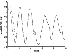
  Figure 9: Positions of two-link robot

  

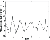
  Figure 10: Velocities of two-link robot

  The above observers provide a simple alternative to current design methods [see e.g., Berghuis and Nijmeyer, 1993; Marino and Tomei, 1995], and guarantees local (for bounded velocities and time-varing inputs) exponential convergence.

  Note that Theoreom 5 can also be used to bound the diverging behavior, caused by the concave inertia when the robot arm is pointing inwards, of the double inverted pendulum, when no damping or stabilizing potential force is applied. $\Box$

• Example 5.4

  : Biology found a solution to the problem that a time-varying supporting torque can destabilize a system.

  Recently, there has been considerable interest in analyzing feedback controllers for biological motor control systems as combinations of simpler elements, or motion primitives. For instance [4] and [16] stimulate a small number of areas (A, B, C, and D) in a frog’s spinal cord and measure the resulting torque angle relations.

  Force fields seem to add when different areas are stimulated at the same time so that [4] and [16] propose the following biological control inputs

  $$f_{i}=-\sum_{l=1}^{n}k_{l}(t)f_{il}(q^{j})$$

  where each single torque $k_{l}(t)f_{il}(q^{j})$ results from the stimulation of area $l$ in the spinal cord. With force measurements the above authors did show that the covariant derivative $\frac{\partial f_{il}}{\partial x^{p}}+\gamma^{h}_{ip}f_{hl}$ of $f_{il}$ with respect to the inertia tensor of the frog’s leg or body is uniformly positive definite.

  Likely candidates for $k_{i}(t)$ are positive upper and lower bounded sigmoids and pulses and periodic activation patterns.

  Using Theorem 5 or the discussion in Example 10 with sufficient damping then allows to compute a maximal $\dot{q}^{j}$ for which exponential convergence to a single motion is guaranteed.

  Note that the achievement of tracking control with a proportional gain $k_{l}(t)$ rather than an additional supporting force as in Example 10 has the advantage that the supporting force has no impact on the contraction behavior anymore. $\Box$

6 Concluding remarks

The research in this paper can be extended in several directions, as the development suggests.

Some of the extensions will likely require the combination of the above results with a simplifying metric pre-transformation, as mentioned in section 3.1. In particular, classical transformation ideas in nonlinear control such as feedback linearization and flatness [6] typically use linear time-invariant target dynamics, while the framework provided in this paper should allow considerably more flexibility. This, combined with the fact that a metric transformation such as $\ \delta{\bf z}={\bf\Theta}\delta{\bf x}\$ need not be integrable (i.e. does not require an explicit ${\bf z}$ to exist), could potentially lead to useful generalisations of these methods.

Acknowledgement  The authors are grateful to Yong Zhao for performing the simulations and for stimulating discussions, and to Wei Wang for thoughtful comments and suggestions.

References

- [1] Aghannan, N., Rouchon, P., An Intrinsic Observer for a Class of Lagrangian Systems, I.E.E.E. Trans. Aut. Control, 48(6) (2003).
- [2] Aylward E., Parrilo P., and J.J.E. Slotine, Algorithmic search for contraction metrics via SOS programming, submitted to the 2006 American Control Conference.
- [3] Bertsekas, D., and Tsitsiklis, J., Parallel and distributed computation: numerical methods, Prentice-Hall, 1989.
- [4] Bizzi E., Giszter S.F., Loeb E., Mussa-Ivaldi F.A., Saltiel P., Trends in Neurosciences. Review 18:442, 1995.
- [5] Bryson A., Ho, Y., Applied Optimal Control, Taylor and Francis, 1975.
- [6] Fliess M., Levine J., Martin Ph., and Rouchon P., Flatness and defect of nonlinear systems: introductory theory and examples. Int. J. Control, 61(6), 1995.
- [7] Goldstein H., Classical Mechanics, Addison Wesley, 1980.
- [8] Hartmann, P. Ordinary differential equations, John Wiley Sons, New York, 1964.
- [9] Jouffroy J. and J. Opderbecke. Underwater vehicle trajectory estimation using contracting PDE-based observers, American Control Conference, Boston, Ma, 2004.
- [10] Kailath, T., Linear Systems, Prentice Hall, 1980.
- [11] Lewis, D.C., Metric properties of differential equations, American Journal of Mathematics, 71, pp. 294-312, 1949.
- [12] Lohmiller, W., and Slotine, J.J.E., On Contraction Analysis for Nonlinear Systems, Automatica, 34(6), 1998.
- [13] Lohmiller, W., and Slotine, J.J.E., Nonlinear Process Control Using Contraction Theory, A. I. Che. Journal, March 2000.
- [14] Lohmiller, W., and Slotine, J.J.E., Contraction Analysis of Nonlinear Distributed Systems, International Journal Of Control, 78(9), 2005.
- [15] Lovelock D., and Rund, H., Tensors, Differential Forms, and Variational Principles, Dover, 1989.
- [16] Mussa-Ivaldi, F.A., I.E.E.E. International Symposium on Computational Intelligence in Robotics and Automation, 1997.
- [17] Nguyen, T.D., and Egeland, O. Observer Design for a Towed Seismic Cable, American Control Conference, Boston (2004)
- [18] Shamma, J., and Gurdal, A., Dynamic Fictitious Play, Dynamic Gradient Play and Distributed Convergence to Nash Equilibra, IEEE Transactions on Automatic Control, March 2005
- [19] Slotine and Li, Applied Nonlinear Control, Prentice Hall, 1991.
- [20] Zhao, Y., and Slotine, J.J.E., Discrete Nonlinear Observers for Inertial Navigation, Systems and Control Letters, 54(8), 2005.
- [21] The Restricted Three Body Problem, http://www.physics.cornell.edu/ sethna/teaching/sss/jupiter/Web/Rest3Bdy.htm