$q$-Breathers in Fermi-Pasta-Ulam chains: existence, localization and stability

Abstract

The Fermi-Pasta-Ulam (FPU) problem consists of the nonequipartition of energy among normal modes of a weakly anharmonic atomic chain model. In the harmonic limit each normal mode corresponds to a periodic orbit in phase space and is characterized by its wave number $q$. We continue normal modes from the harmonic limit into the FPU parameter regime and obtain persistence of these periodic orbits, termed here $q$-Breathers (QB). They are characterized by time periodicity, exponential localization in the $q$-space of normal modes and linear stability up to a size-dependent threshold amplitude. Trajectories computed in the original FPU setting are perturbations around these exact QB solutions. The QB concept is applicable to other nonlinear lattices as well.

1 Introduction

In the year 1955 E. Fermi, J. Pasta, and S. Ulam (FPU) published their celebrated report on thermalization of arrays of particles connected by weakly nonlinear springs [1]. Instead of the expected equipartition of energy among the normal modes of the systems, FPU observed that energy, initially placed in a low frequency normal mode of the linear problem with a frequency $\omega_{q}$ and a corresponding wave number $q$, stayed almost completely locked within a few neighbour modes, instead of being distributed among all modes of the system. Moreover, recurrence of energy to the originally excited mode was observed. The door was thus opened to study the fundamental physical and mathematical problem of energy equipartition and ergodicity in nonlinear systems, which involves the Kolmogorov-Arnold-Moser (KAM) theorem, dividing thresholds between regular and chaotic dynamics, and soliton bearing integrable models.

From the present perspective, the FPU observation (equally coined FPU problem or FPU paradox) appears to consist of three major ingredients: (FPU-1) for suitable parameter ranges (energy, system size, nonlinearity strength) low frequency excitations are localized in $q$-space of the normal modes; (FPU-2) recurrence of energy to an initially excited low-frequency mode is observed; (FPU-3) different thresholds upon tuning the parameters are observed - a weak stochasticity threshold (WST) which separates regular from chaotic dynamics, yet possibly preserving the localization character in $q$-space, and an equipartition threshold (ET) also coined strong stochasticity threshold separating localized from delocalized dynamics in $q$-space (see [2, 3, 4] for a review).

Two major approaches were developed. The first one, taken by N. Zabusky and M. Kruskal, was to analyze dynamics of the nonlinear chain in the continuum limit, which led to a pioneering observation of solitary waves [5]. It took (FPU-1) as given, and aimed at obtaining quantitative estimates for (FPU-2). A second approach was proposed by F. Izrailev and B. Chirikov [6] who associated energy equipartition with dynamical chaos and aimed at an analytical estimate of the ET by computing the overlap of nonlinear resonances [7] which leads to strong dynamical chaos insuring energy equipartition. Below the threshold the dynamics is regular and, thus, no equipartition should occur. It aimed mainly at (FPU-3). Several other analytical [8, 9] and numerical [10],[11],[12] threshold estimates have been published since, and will be discussed below. Note that similar effects have been observed in many other nonlinear discrete chain or field equations on a finite spatial domain, see e.g. [13].

In this work we show that stable periodic orbits, coined $q$-breathers (QB), persist in the nonlinear FPU chain, which are exponentially localized in $q$-space. The existence of these orbits was first reported in ref.[14]. Stability of these periodic orbits implies that nearby trajectories will be localized in $q$-space as well, and evolve in a nearly regular fashion for long times on submanifolds similar to low-dimensional tori in phase space. Recurrence times - to come close to an initial point on such a torus again - will be much shorter than the general recurrence times estimates for the dynamics on an assumed KAM torus in the whole phase space. That follows from the fact that a KAM torus in general will have the dimension equivalent to the number of degrees of freedom, and thus much larger than the effective dimension of the perturbed $q$-breather evolution. Upon tuning the parameters of the system, QBs will turn from stable to unstable at certain threshold values, allowing for low-dimensional chaotic evolution of nearby trajectories. The localization length in $q$-space depends on these parameters as well, and at critical parameter values QBs delocalize, leading to equipartition. The $q$-breather concept allows thus to address simultaneously all three FPU ingredients. At the same time it can be extended to completely different lattice systems and even to nonlinear field equations.

In the present work we construct QBs continuing them from the linear case and study their properties both numerically and by an analytical asymptotic calculation. We compare the thresholds of QB existence and stability to the various stochasticity thresholds mentioned above. Finally we show the persistence of QBs in thermal equilibrium and during long transient processes.

2 The model

The FPU system is a chain of $N$ equal masses coupled by nonlinear springs with the equations of motion containing quadratic (the $\alpha$-model)

$$\ddot{x}_{n}=(x_{n+1}-2x_{n}+x_{n-1})\\ +\alpha[(x_{n+1}-x_{n})^{2}-(x_{n}-x_{n-1})^{2}]$$ (1)

or cubic (the $\beta$-model)

$$\ddot{x}_{n}=(x_{n+1}-2x_{n}+x_{n-1})+\beta[(x_{n+1}-x_{n})^{3}-(x_{n}-x_{n-1})^{3}]$$ (2)

interaction terms, where $x_{n}$ is the displacement of the $n$-th particle from its original position, and fixed boundary conditions are taken $x_{0}=x_{N+1}=0$. A canonical transformation

$$x_{n}(t)=\sqrt{\frac{2}{N+1}}\sum\limits_{q=1}^{N}Q_{q}(t)\sin{\left(\frac{\pi qn}{N+1}\right)}$$ (3)

takes into the reciprocal wavenumber space with $N$ normal mode coordinates $Q_{q}(t)$. The equations of motion then read

$$\ddot{Q}_{q}+\omega_{q}^{2}Q_{q}=-\frac{\alpha}{\sqrt{2(N+1)}}\sum\limits_{l,m=1}^{N}\omega_{q}\omega_{l}\omega_{m}B_{q,l,m}Q_{l}Q_{m}$$ (4)

for the FPU-$\alpha$ chain (1) and

$$\ddot{Q}_{q}+\omega_{q}^{2}Q_{q}=-\frac{\beta}{2(N+1)}\sum\limits_{l,m,n=1}^{N}\omega_{q}\omega_{l}\omega_{m}\omega_{n}C_{q,l,m,n}Q_{l}Q_{m}Q_{n}$$ (5)

for the FPU-$\beta$ chain (2). Here the coupling coefficients $B_{q,l,m}$ and $C_{q,l,m,n}$ are given by

$$B_{q,l,m}=\sum\limits_{\pm}(\delta_{q\pm l\pm m,0}-\delta_{q\pm l\pm m,2(N+1)})\mbox{,}$$ (6)

$$C_{q,l,m,n}=\sum\limits_{\pm}(\delta_{q\pm l\pm m\pm n,0}-\delta_{q\pm l\pm m\pm n,2(N+1)}-\delta_{q\pm l\pm m\pm n,-2(N+1)})\mbox{.}$$ (7)

The sum in (6) and (7) is taken over all 4 or 8 combinations of signs, respectively. The normal mode frequencies

$$\omega_{q}=2\sin\frac{\pi q}{2(N+1)}\mbox{.}$$ (8)

are nondegenerate.

3 A crosslink to discrete breathers

The system of equations (4),(5) corresponds to a network of oscillators with different eigenfrequencies. These oscillators are interacting with each other via nonlinear interaction terms, yet being long-ranged in $q$-space. Let us discuss the relation of this problem to the wellknown field of discrete breathers [15, 16, 17].

Neglecting the nonlinear terms in the equations of motion the $q$-oscillators get decoupled, each conserving its energy

$$E_{q}=\frac{1}{2}\left(\dot{Q}_{q}^{2}+\omega_{q}^{2}Q_{q}^{2}\right)$$ (9)

in time. Especially, we may consider the excitation of only one of the $q$-oscillators, i.e. $E_{q}\neq 0$ for $q\equiv q_{0}$ only. Such excitations are trivial time-periodic and $q$-localized solutions (QBs) for $\alpha=\beta=0$.

This setting is similar to the case of discrete breathers (DB), that are time-periodic and spatially localized excitations e.g. on networks of interacting identical anharmonic oscillators, which survive continuation from the trivial limit of zero coupling [18]. Notably, DBs exist also in FPU lattices [17] and existence proofs have been obtained as well [19, 20, 21]. The reason for the generic existence of DBs is two-fold: the nonlinearity of each oscillator allows to tune its excitation frequency out of resonance with other nonexcited oscillators. The case of a linear coupling on the lattice ensures a bound spectrum of small amplitude plane waves, and thus allows for the escape of resonances of a DB frequency and its higher harmonics with that spectrum. The spatial localization of DBs in such a case is typically exponential for short-range interactions [15]. Among the wealth of theoretical results we stress two here. First, if the coupling on the lattice is short-ranged but purely nonlinear, the DB localizes in space superexponentially [22]. Second, if the coupling is algebraically decaying on the lattice, DBs localize only algebraically as well [23].

Let us compare these findings to the $q$-breather setting. The nonidentical $q$-oscillators are harmonic, but with frequencies being nonresonant. That ensures continuation of a trivial QB orbit from zero nonlinearity into the domain of nonzero nonlinearity. Indeed, similar to the existence proof of discrete breathers by MacKay and Aubry [18] by continuation from the trivial uncoupled limit, we can start at zero nonlinearity and excite mode $q_{0}$ to energy $E_{q_{0}}$, with all other modes at rest. By properly choosing the origin of time the solution will be time-periodic and time-reversible, i.e. $\hat{Q}_{q}(t+T)=\hat{Q}_{q}(t)$, $\hat{Q}_{q}(t)=\hat{Q}_{q}(-t)$. Following [18] we first observe that

$$u_{q}(t)=\ddot{U}_{q}+\omega_{q}^{2}U_{q}+\frac{\alpha}{\sqrt{2(N+1)}}\sum\limits_{l,m=1}^{N}\omega_{q}\omega_{l}\omega_{m}B_{q,l,m}U_{l}U_{m}$$ (10)

maps any choice of time-periodic time-reversible functions $U_{q}(t;T)$ onto time-periodic and time-reversible functions $u_{q}(t;T)$ where the period $T$ is variable. For $\alpha=0$ the particular choice $U_{q}(t;T)=\hat{Q}_{q}(t)$ and $T=2\pi/\omega_{q_{0}}$ ensures that $u_{q}(t;T)=0$, i.e. the map (10) of time-periodic and time-reversible functions (spanning a Banach space) contains a zero. In the next step we have to check whether the map (10) is invertible at $\alpha=0$. Following MacKay and Aubry [18] invertibility is trivially obeyed for all $q\neq q_{0}$ in (10), provided $m2\pi/T\neq\omega_{q}$. This nonresonance condition is generically fulfilled for any finite lattice size $N$ and a period $T=2\pi/\omega_{q_{0}}+\epsilon$ where $\epsilon$ is a small but finite number of the order $1/N$. As for $q_{0}$ itself, we conclude that invertibility is given provided we demand e.g. fixing the value $U_{q_{0}}(t=0;T)$ to a given nonzero number. With these possibilities we arrive at the full invertibility of (10) at $\alpha=0$. We may then conclude (and skip the full derivation which follows [18]) that the Implicit Function Theorem can be applied, and the zero of (10) for $\alpha=0$ will persist up to some nonzero value of $\alpha$. Of course the same procedure can be applied to the FPU-$\beta$ model.

As for their degree of localization in $q$-space (if any), the above results on DBs suggest that two mechanisms counteract: purely nonlinear interaction favours stronger than exponential localization, while long-range interaction tends to delocalize the QB. We also recall that the seemingly simple problem of periodic motion of a classical particle in an anharmonic potential of the FPU type follows from the differential equation

$$\ddot{x}=-x-\alpha x^{2}-\beta x^{3}\;.$$ (11)

Bounded motion at some energy $E$ yields a solution which is periodic with some period $T(E)=2\pi/\Omega$ and can be represented by a Fourier series

$$x(t)=\sum_{k}A_{k}{\rm e}^{ik\Omega t}$$ (12)

which leads to algebraic equations for the Fourier coefficients $A_{k}$

$$A_{k}=k^{2}\Omega^{2}A_{k}-\alpha\sum_{k_{1}}A_{k_{1}}A_{k-k_{1}}-\beta\sum_{k_{1},k_{2}}A_{k_{1}}A_{k_{2}}A_{k-k_{1}-k_{2}}\;.$$ (13)

Note that the equations (13) have similar properties as compared to (4),(5) - interaction between the Fourier coefficients is nonlinear but long ranged. Yet it is well known that the bounded solutions (12) to (11) are analytic functions $x(t)$ and thus the Fourier series coefficients $A_{k}$ converge exponentially fast with $k$ [25].

Let us summarize this chapter with stating that from a mathematical point of view $q$-breather existence and their properties can be treated in a similar way to the methodology of discrete breather theory. The two different types of excitations, localized in real space and localized in reciprocal $q$-space, have much in common when represented in their natural phase space basis choice. Both representations are connected to each other by a simple canonical transformation, which is nothing but a rotation of the phase space basis. In the following we will use analytical and computational tools developed for discrete breathers and analyze the properties of $q$-breathers.

4 q-Breathers in the $\alpha$-FPU system

4.1 Numerical results

Let us consider the $\alpha$-model and start with showing the evolution of the original FPU trajectory for $\alpha=0.25$, $N=32$ and an energy $E=0.077$ placed initially into the mode with $q_{0}=1$. We plot the time dependence of the mode energies $E_{q}(t)$ in Fig.1 for the first five modes.

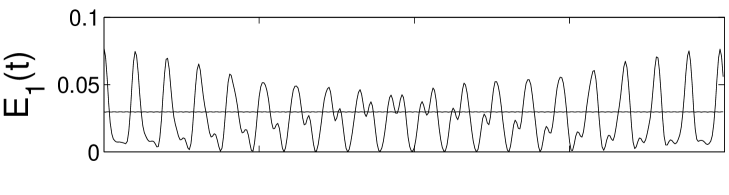
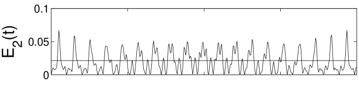
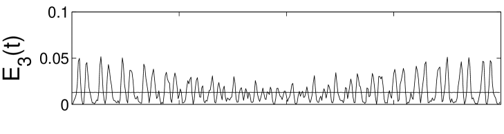
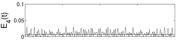
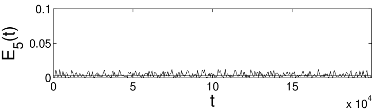
Figure 1: Evolution of the linear mode energies for the first five modes on a large timescale for (i) the original FPU trajectory for $\alpha=0.25,E=0.077,N=32$ [1] (oscillating curves) and (ii) the exact QB solution (almost straight lines).

The period of the slowest ($q_{0}=1$) harmonic mode is $T_{1}=2\pi/\omega_{1}\approx 66.02$. We nicely observe slow processes of redistribution of mode energies, recurrences and also even slower modulations of recurrence amplitudes on time scales of the order of $10^{5}$. Note also that on time scales comparable to $T_{1}$ all mode energies show small additional oscillations - and it is easy to see that they correspond to frequencies which are multiples of $\omega_{1}$. The localization in $q$-space is also nicely observed, with the maximum of $E_{5}$ being eight times smaller than that of $E_{1}$.

In order to construct a $q$-breather, let us choose first $\alpha=0$, excite a normal mode with $q=q_{0}$ to the energy $E_{q_{0}}=E$ and let all other $q$-oscillators be at rest. With that we arrive at a unique periodic orbit in the phase space of the FPU model. We expect that the orbit will stay localized in $q$-space at least up to some critical nonzero value of $\alpha$ (and similarly for the $\beta$-model [26]). We proceed with a series of successful numerical experiments continuing periodic orbits of the linear chain to nonzero nonlinearity. These orbits as well as their Floquet spectra can be calculated using well developed computational tools [15] for exploring periodic orbits.

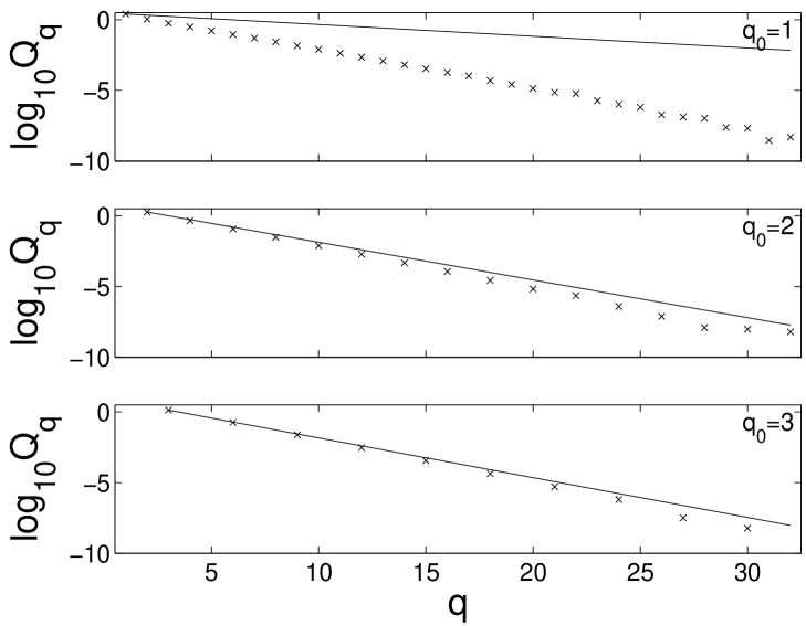
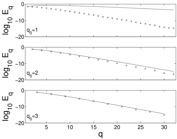
Figure 2: Snapshots of the linear mode coordinates $Q_{q}$ (symbols) along with analytical predictions (lines) for QBs with $q_{0}=1,2,3$ for $\alpha=0.25,E=0.077,N=32$, at the moment when all velocities $\dot{Q}_{q}$ equal zero. Some modes have zero contributions and their corresponding symbols are not plotted here.

Figure 3: Distributions of the linear mode energies $E_{q}$ in $q-$space for QBs with $q_{0}=1,2,3$ for $\alpha=0.25,E=0.077,N=32$.

We choose a Poincaré section plane $\{x_{s}=0,\dot{x}_{s}>0\}$, where $s=[2(N+1)/q_{0}]$ corresponds to an antinode of the mode $Q_{q_{0}}$. We map the plane $\vec{y}$ (all phase variables excluding $x_{s}$) onto itself integrating the equations of motion (1) until the trajectory crosses the plane again: $\vec{y}^{n+1}=\vec{\mathcal{F}}(\vec{y}^{n})$. A periodic orbit of the FPU chain corresponds to a fixed point of the generated map. As the initial guess we use the point corresponding to the $q_{0}$-th linear mode: $\dot{x}_{n}(0)=\sqrt{\frac{2}{N+1}}\dot{Q}_{q_{0}}(0)\sin{\left(\frac{\pi q_{0}n}{N+1}\right)}$, $x_{n}(0)=0$. The vector function $\vec{\mathcal{G}}=\vec{\mathcal{F}}(\vec{y})-\vec{y}$ is used to calculate the Newton matrix $\mathcal{N}=\partial{\mathcal{G}(\vec{y})_{i}}/\partial y_{j}$. We use a Gauss method to solve the equations $\vec{\mathcal{G}}(\vec{y})={\mathcal{N}}(\vec{y}-\vec{y}\ ^{\prime})$ for the new iteration $\vec{y}\ ^{\prime}$ and do final corrections to adjust the correct total energy $E$. The iteration procedure continues until the required accuracy $\varepsilon$ is obtained: $||\vec{\mathcal{F}}(\vec{y})-\vec{y}||/||\vec{y}||<\varepsilon$ (we have varied $\varepsilon$ from $10^{-5}$ to $10^{-8}$), where $||\vec{y}||=\max\{|y_{i}|\}$. We also note that all periodic orbits computed here are invariant under time reversal, which means that there exist times $t_{0}$ when $Q_{q}(t_{0}+t)=Q_{q}(t_{0}-t)$ for all $q$. Since mode velocities vanish at these times, a QB can be also computed e.g. by initially choosing all mode velocities to zero, and integrating until $\dot{Q}_{q_{0}}$ vanishes again at the same sign of $Q_{q_{0}}$ as it was at the starting point. Then the fixed point of the corresponding map of the mode coordinates only suffices to obtain an exact periodic solution.

We have used one of the original parameter sets of the FPU$-\alpha$ study $\alpha=0.25,E=0.077,N=32$ [1] to find stable $q$-localized QB solutions with most of the energy concentrated in the mode $q_{0}=1$ (and added the cases $q_{0}=2,3$ for comparison, see Fig.3,3). Note, that in (6) $2(N+1)$ is always a multiple of 2, and in the particular case of $N=32$ it is also a multiple of 3. Then, for $q_{0}=2$ and $q_{0}=3$ only modes with $q$ being a multiple of $q_{0}$ are excited. Let us discuss the properties of the found solutions in some detail. In contrast to the original FPU trajectories, the QB is characterized by mode energies being almost constant in time. The straight lines in Fig.1 compare the mode energies on the QB with $q_{0}=1$ with the FPU trajectory. The period of the QB solutions is very close to the corresponding period $T_{q_{0}}=2\pi/\omega_{q_{0}}$ of the harmonic mode which is continued. During one QB period of oscillations a relatively small energy interchange between the modes (of the order of 2 percent) is observed (Fig.5(a-c)).

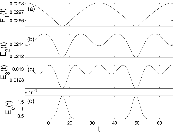
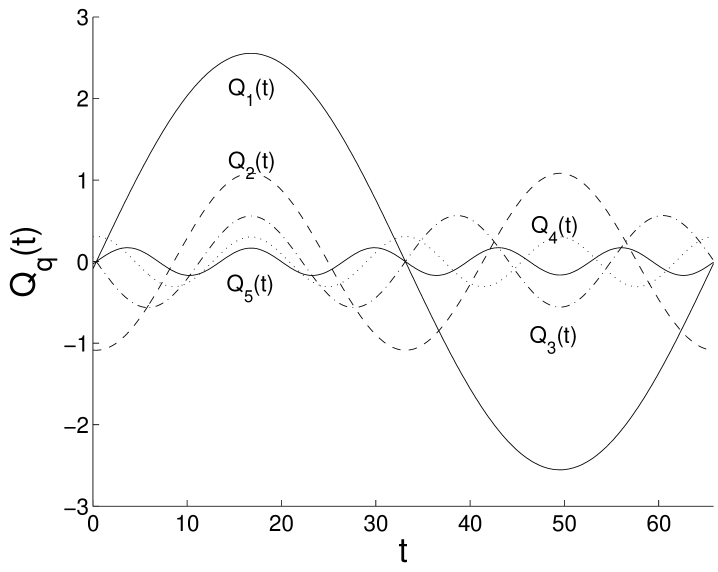
Figure 4: Evolution of the linear mode energies (a) $E_{1}$, (b) $E_{2}$, (c) $E_{3}$ and the energy of nonlinear coupling (d) $E_{c}$ (see the text for definition) for the QB with $q_{0}=1,\alpha=0.25,E=0.077,N=32$.

Figure 5: Evolution of the linear mode coordinates $Q_{1,2,3,4,5}$ for the QB with $q_{0}=1,\alpha=0.25,E=0.077,N=32$.

with frequencies which correspond to multiples of the QB frequency - just like the small fluctuations of the mode energies for the FPU trajectory mentioned above. There are well defined intervals during which the energy of nonlinear coupling energy $E_{c}=E_{tot}-\sum_{q=1}^{N}E_{q}$ ($E_{tot}$ being the full energy of the chain) increases sharply, yet being overall very small (between 1 and 3 percent of the total energy, see Fig.5(d)). In Fig.5 we show the time dependence of the first five mode coordinates on the QB with $q_{0}=1$. The time reversal symmetry is nicely observed (although not used for construction) at times $t_{0}\approx 17,49$. Note also that while $Q_{1}$ oscillates predominantly with the main QB frequency $\Omega_{QB}$ which is close to $\omega_{1}$, the second mode $Q_{2}$ is dominated by $2\Omega_{QB}$, the third one $Q_{3}$ by $3\Omega_{QB}$ etc.

We conclude the numerical results on the $\alpha$-FPU case with QB solutions for $q_{0}=1$, $E=0.077$ and various values of $\alpha$ up to $\alpha=0.8$, which are shown in Fig.6.

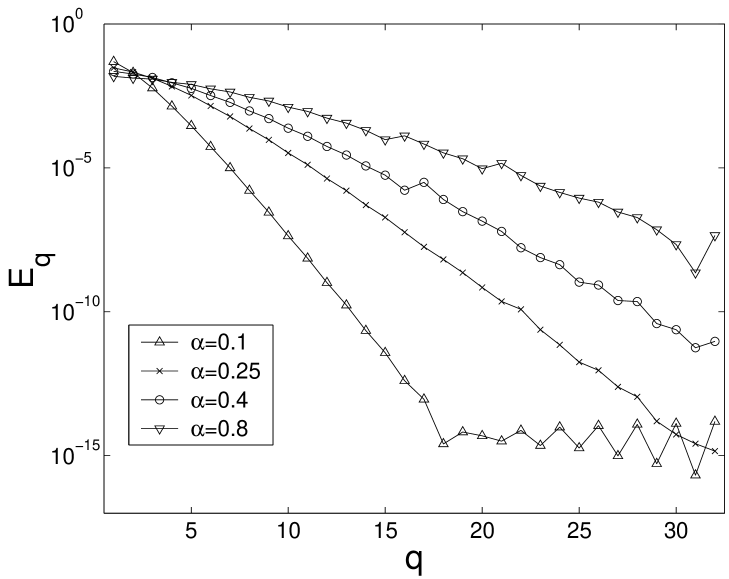
Figure 6: Distributions of the linear mode energies $E_{q}$ for $\alpha=0.1,0.25,0.4$ and $0.8$ for QBs with $q_{0}=1,E=0.077,N=32$.

We observe that the localization length increases with increasing $\alpha$, so there is a clear tendency towards an equipartition threshold.

4.2 Estimating the localization length

To demonstrate localization of a QB solution in $q$-space analytically, we expand the solution to (4) into an asymptotic series with respect to the small parameter $\sigma=\alpha/\sqrt{2(N+1)}$:

$$Q_{q}(t)=\sum_{n=0}^{\infty}\sigma^{n}Q^{(n)}_{q}(t)\mbox{.}$$ (14)

Inserting this expansion into (4), we obtain equations for the variables $Q^{(n)}_{q}(t)$. The equation for the zero order $n=0$ reads

$$\ddot{Q}^{(0)}_{q}+\omega_{q}^{2}Q^{(0)}_{q}=0\mbox{,}$$ (15)

and for $n>0$

$$\ddot{Q}^{(n)}_{q}+\omega_{q}^{2}Q^{(n)}_{q}=-\omega_{q}\sum_{l,m=1}^{N}\omega_{l}\omega_{m}B_{qlm}\mspace{-18.0mu}\sum_{\begin{subarray}{c}n_{1,2}=0\\ n_{1}+n_{2}=n-1\end{subarray}}^{n-1}\mspace{-18.0mu}Q^{(n_{1})}_{l}Q^{(n_{2})}_{m}\mbox{.}$$ (16)

As the zero-order approximation we take a single-mode solution to (15) with $Q^{(0)}_{q}(t)\neq 0$ only for $q=q_{0}$:

$$Q_{q}^{(0)}=\delta_{q,q_{0}}A_{q_{0}}\cos{\omega_{q_{0}}t}\mbox{.}$$ (17)

Consider the first-order equations (case $n=1$ in (16)). The right-hand part in (16) contains only one nonzero term corresponding to $l=m=q_{0}$, $n_{1}=n_{2}=0$. The coefficient $B_{qlm}$ here is non-zero only for $q=q_{0}$ and $q=2q_{0}$ (here we assume $2q_{0}\leq N$, so that the second Kronecker symbol in (6) always equals zero). Thus, in the first order the only variables different from zero are $Q^{(1)}_{q_{0}}(t)$ and $Q^{(1)}_{2q_{0}}(t)$.

Similarly, for $n=2$, provided $3q_{0}\leq N$, we get $Q^{(2)}_{q}(t)\neq 0$ for $q=q_{0},2q_{0},3q_{0}$ only.

The above allows us to formulate the following proposition.

In the $(k-1)$th order of asymptotic expansion, provided $kq_{0}\leq N$, variables $Q^{(k-1)}_{q}(t)$ differ from zero only for $q=q_{0},2q_{0},\dots,kq_{0}$:

$$Q^{(k-1)}_{q}(t)=0\quad\forall q\notin\{q_{0},2q_{0},\dots,kq_{0}\}\mbox{.}$$ (18a)

It means, that the first non-zero expansion term for a mode $$q=kq_{0} k-1$$ is of the order :

$$Q^{(m)}_{kq_{0}}(t)=0\quad\forall m<k-1\mbox{.}$$ (18b)

In Appendix A we prove this statement by the method of mathematical induction and approximate the first non-zero term for a mode $q=kq_{0}$ at $kq_{0}\ll N$:

$$Q^{(k-1)}_{kq_{0}}(t)=A_{kq_{0}}\left(\cos k\omega_{q_{0}}t+O\left((kq_{0}/N)^{2}\right)\right)\mbox{,}$$ (19a)

where

$$A_{kq_{0}}=\frac{A_{q_{0}}^{k}}{\omega_{q_{0}}^{k-1}}\mbox{.}$$ (19b)

Ignored expansion terms lead to shifting the QB orbit frequency and next-order corrections to its shape.

Multiplying (19) by $\sigma^{k-1}$ and inserting it into (9), we approximate the mode energies as

$$E_{kq_{0}}=k^{2}\gamma^{k-1}E_{q_{0}}\cdot\left(1+O\left((kq_{0}/N)^{2}\right)\right)\left(1+O(\sigma)\right)\mbox{,}$$ (20a)

where

$$\gamma=\frac{\alpha^{2}(N+1)^{3}E_{q_{0}}}{\pi^{4}q_{0}^{4}}\mbox{.}$$ (20b)

Note, that although mode energies are not strictly conserved in time, their variation is small, being limited to the orders of magnitude indicated in (20a) in parentheses (cf. Fig.5). We arrive at an exponential decay in $q$-space dressed with a power law:

$$\ln(E_{q})=2\ln(\frac{q}{q_{0}})+\frac{q}{q_{0}}\ln\gamma+\ln\left(\frac{E_{q_{0}}}{\gamma}\right)$$ (21)

with exponent $q_{0}^{-1}\ln\gamma$ for the exponential part. The predicted decay (20) fits nicely with a computed QB with $q_{0}=1$ and $\alpha=0.025$ as shown in [14]. In Figs.3,3 we compare (20) with the numerical results for $\alpha=0.25$ and $q_{0}=1,2,3$. While $q_{1}$ shows that the analytical results underestimate the degree of localization with increasing $\alpha$, we note that it does even at these values $\alpha$ better for larger values of $q_{0}$.

The calculation described is expected to fail at $\gamma$ close to or greater than one, when (20) does not support $q$-space localization. At the same time the comparison with the numerical results shows that higher order corrections to the analytical decay law extend the region of QB localization. Thus we estimate a lower bound for the QB delocalization threshold energy $E^{loc}$ as

$$E^{loc}=\pi^{4}\alpha^{-2}(N+1)^{-3}q_{0}^{4}\mbox{.}$$ (22)

The scaling behaviour is in good agreement with an analytical estimation of the equipartition threshold in the $\alpha$-model due to second order nonlinear resonance overlap, suggested in [9], which reads $\alpha^{2}EN^{3}\approx q_{0}^{4}$.

Finally we stress an even closer relation between the localization of $q$-breathers within the used perturbation theory and the Fourier series convergence of analytic periodic functions (11),(12),(13). One arrives from the QB problem to these equations by simply assuming $\omega_{q}=const$.

4.3 Stability of $q$-breathers in the $\alpha$-FPU system

An important problem is the stability of QBs. For computing linear stability of an orbit $\hat{Q}_{q}(t)$, the phase space flow around it is linearized by making a replacement

$$Q_{q}=\hat{Q}_{q}(t)+\xi_{q}$$ (23)

in the equations of motion (5) and subsequent linearizing the resulting equations with respect to $\xi_{q}$. Orbit stability is then characterized by the eigenvalues of the Floquet matrix, which defines the linear transformation of small deviations $\xi_{q}$ by the linearized equations over one period of the orbit. If all eigenvalues $\mu_{j}$ have the absolute value one, the orbit is stable, otherwise it is unstable [15, 16].

All QB solutions presented in this section are linearly stable, i.e. all eigenvalues of the Floquet matrix which characterizes the linearized phase space flow around the QB orbits reside on the unit circle. This is at variance with the case of the $\beta$-FPU model, which will be discussed below.

5 $\beta$-FPU system

5.1 Numerical results

Launching an FPU trajectory by exciting a single low-frequency mode leads to similar observations as for the $\alpha$-model. Again energy is localized in $q$-space on a few modes, sometimes coined natural packets [29], which again persists for very long times.

It is possible to construct QBs in the $\beta$-FPU model, following the same way as described above for the $\alpha$-model.

For numerical calculation we use a modified scheme. The section plane is defined in the $q$-space as $\{Q_{q_{0}}=0,\dot{Q}_{q_{0}}>0\}$. It is parametrized as $\vec{r}\equiv\{\dot{Q}_{q},q\neq q_{0}\}$. The even coupling potential and fixed boundary conditions enable us to introduce an additional constraint $Q_{q}(t=0)=0$, and the velocity $\dot{Q}_{q_{0}}$ is obtained using the condition of energy conservation $\dot{Q}_{q_{0}}(t=0)=\sqrt{2E-\sum_{q\neq q_{0}}\dot{Q}_{q}^{2}(t=0)}$. As in the case of the $\alpha$-model, the QB is searched as a fixpoint of the mapping $\vec{r}^{n+1}=\vec{\mathcal{F}}(\vec{r}^{n})$.

We obtain QBs which are exponentially localized in $q$-space (Fig.7). The smaller $\beta$, the faster is the decay of the energy distribution with increasing wave number $q$. Note, that due to the parity symmetry of the $\beta$-model (Eq.(2) is invariant under $x_{n}\rightarrow-x_{n}$ for all $n$) only odd $q$-modes are excited by the $q_{0}=3$ mode and get coupled [28]. This follows also from the coupling matrix (7).

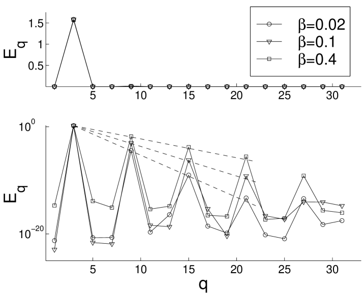
Figure 7: Energy distributions between $q$-modes in QBs for different nonlinear coupling coefficients $\beta$ versus $q$ in linear and log scales with analytical estimations of the QBs exponential localization (dashed lines). Parameters are $E=1.58$, $q_{0}=3$, $N=32$. Only odd modes are shown (see text). The symbols for $q\neq 3,9,15,21,27$ represent upper bounds, the real mode energies might be even less. Note that QBs persist even far beyond the stability threshold (see Fig.8).

5.2 Estimating the localization length

In the analytical computation the solution to (5) is expanded in powers of a small parameter $\rho=\frac{\beta}{2(N+1)}$. In the $n$-th order of expansion variables $Q^{(n)}_{q}$ differ from zero at $q=q_{0},3q_{0},\dots,(2n+1)q_{0}$ only. Then the first non-zero expansion term for a mode $(2n+1)q_{0}$ is of the order $n$. Using the same approach of mathematical induction as described in Appendix A, mode energies in a QB are approximated as follows:

$$E_{(2k+1)q_{0}}=\lambda^{k}E_{q_{0}}\cdot\left(1+O\left(((2k+1)q_{0}/N)^{2}\right)\right)\left(1+O(\rho)\right)\mbox{,}$$ (24a)

where

$$\lambda=\frac{9\beta^{2}E_{q_{0}}^{2}(N+1)^{2}}{64\pi^{4}q_{0}^{4}}\mbox{.}$$ (24b)

Again, time variation of mode energies is limited to the orders of magnitude indicated in (24a). We arrive at a pure exponential decay

$$\ln(E_{q})=\ln E_{q_{0}}+\frac{1}{2}(\frac{q}{q_{0}}-1)\ln\lambda$$ (25)

with exponent $(2q_{0})^{-1}\ln\lambda$. The predicted decay (24) fits nicely with the computed QBs in Fig.7.

The QB delocalization threshold is then estimated as

$$E_{q_{0}}=\frac{8}{3}\pi^{2}q_{0}^{2}\beta^{-1}(N+1)^{-1}\mbox{.}$$ (26)

The scaling behaviour is in good agreement with an analytical estimation of the equipartition threshold in the $\beta$-model due to second order nonlinear resonance overlap, obtained in [9], which reads $\beta EN\approx q_{0}^{2}$ .

5.3 Stability of $q$-breathers for the $\beta$-FPU model

First, we study QB stability by computing the Floquet matrix numerically and diagonalizing it. In Fig.8 we plot the absolute values of the Floquet eigenvalues of the computed QBs versus $\beta$ for different system sizes $N$. QBs are stable for sufficiently weak nonlinearities (all eigenvalues have absolute value 1). When $\beta$ exceeds a certain threshold two eigenvalues get absolute values larger than unity (and, correspondingly, another two get absolute values less than unity) and a QB becomes unstable. Remarkably, unstable QBs can be traced far beyond the stability threshold, and moreover, they retain their exponential localization in $q$-space (Fig.7). As $\beta$ is increased further, new bifurcations of the same type are observed.

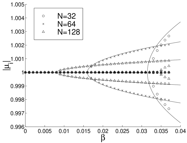
Figure 8: Absolute values of Floquet multipliers $|\mu_{i}|$ of QBs with the energy $E=1.58$ and $q_{0}=3$ and different $N$ versus $\beta$. Symbols: numerical results, lines: analytical results.

To study QB stability analytically in the first-order approximation, we write down the QB solution in the form

$$\hat{Q}_{q}(t)=\delta_{qq_{0}}A\cos\hat{\omega}t+O(\rho)\mbox{,}$$ (27)

where $\hat{\omega}$ is the QB frequency, slightly shifted from $\omega_{q_{0}}$ due to nonlinearity. The residual term $O(\rho)$ includes corrections to the QB orbit shape by expansion terms of order one and higher.

The first-order correction to the QB frequency is determined by secularity caused by resonant nonlinear self-forcing of the mode $q_{0}$ in the first order of expansion:

$$\ddot{Q}^{(1)}_{q_{0}}+\omega_{q_{0}}^{2}Q^{(1)}_{q_{0}}=-3\omega_{q_{0}}^{4}{Q^{(0)}_{q_{0}}}^{3}$$ (28)

This equation is identical to that of an isolated oscillator with cubic nonlinearity (Duffing oscillator). The well-known expression of nonlinear frequency shifting in the Duffing oscillator then yields

$$\hat{\omega}=\omega_{q_{0}}\left(1+\frac{9\beta E_{q_{0}}}{8(N+1)}+O(\rho^{2})\right)$$ (29)

Linearizing equations of motion (5) around (27) according to (23), we arrive at a Mathieu equation (see Appendix B), which finally leads to an estimation of the Floquet multipliers which leave the unit circle due to a primary parametric resonance and cause instability:

$$|\mu_{j_{1}j_{2}}|=1\pm\frac{\pi^{3}}{4(N+1)^{2}}\sqrt{R-1+O(\frac{1}{N^{2}})}$$ (30)

where

$$R=6\beta E_{q_{0}}(N+1)/\pi^{2}\;.$$ (31)

The bifurcation occurs at $R=1+O(1/N^{2})$. This instability threshold coincides with the criterion of transition to weak chaos reported by De Luca et al. [8]. Note, that (30) does not contain the principal mode number $q_{0}$. Below the stability threshold (except for possible small high-order resonance zones) a set of stable QB modes exists. In the thermodynamical limit $N\to\infty$, however, the energy of stable QBs tends to zero. Note that according to our analytical (Appendix B) and numerical results the instability modes correspond to $q^{\prime}=q_{0}\pm 1$ and are even modes if $q_{0}$ is odd and vice versa. The observed instability is thus connected to a lowering of the symmetry of the higher symmetry QB. That has been also observed to be the driving pathway for the onset of low-dimensional stochasticity in the FPU trajectory at the weak chaos transition [8],[30], where the FPU trajectory acquires chaotic components in the time evolution, while still being localized in $q$-space.

The result (30) is plotted in Fig.8 with solid lines for $N=32$, 64 and 128, demonstrating good agreement with the numerical results. The agreement improves with increasing $N$ [31].

Driscoll and O’Neil studied the instability of a single soliton in the continuum mKdV limit of the $\beta$-FPU model [32] with periodic boundary conditions. A stability threshold obtained within the mKdV equation will qualitatively or semiquantitatively agree with the correct value obtained for the discrete chain, if the instability sets in for QBs which do not contain significant short wavelength components. The relation between single soliton and QB stability is less clear, since in the limit of vanishing nonlinearity QBs in chains or field equations with periodic boundary conditions correspond to standing waves, while single solitons transform into plane (running) waves.

We conclude this section with the observation that the stability (31) and delocalization (26) threshold estimates for QBs contain a unique parameter $\beta EN$ where $E$ is the total energy, at variance with scaling estimates for the transition times to equipartition [33], which obtain $\beta E/N$ instead.

6 QBs and the FPU-trajectory for the $\alpha$-FPU model

Departing from the the QB orbit in phase space in the direction of the initial condition of the FPU trajectory implies adding to the QB solution, which is localized in $q$-space, a perturbation, which is localized in q-space as well. The perturbed trajectory will evolve essentially on a low-dimensional torus in phase space, whose dimension will correspond to the number of modes excited on the QB orbit - e.g. for $\alpha=0.25$ and $q_{0}=1$ about four or five. In Fig.9 we compare snapshots of displacements at different times obtained for the original FPU trajectory in [1] and for the numerically exact QB solution from Fig.3 for $\alpha=0.25$ and observe similar evolution patterns (see also Ref. [12]).

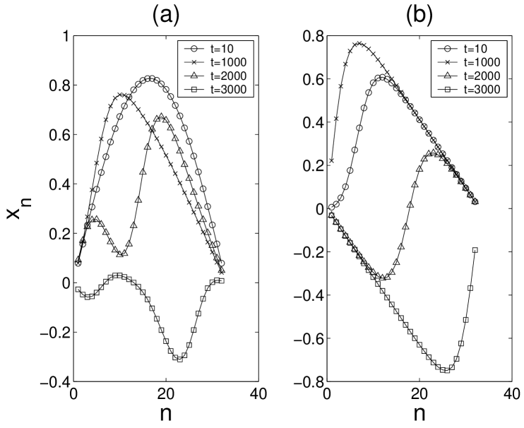
Figure 9: Snapshots of displacements (a) of the original FPU trajectory for $\alpha=0.25,E=0.077,N=32$ [1] and (b) of the corresponding exact QB solution from Fig.3 taken at different times.

Moreover, we took a series of points on a line which connected initial conditions of the FPU trajectory ($E_{q\neq 1}=0$) with the numerically exact QB solution from Fig.3. For each of these points we integrated the corresponding trajectory and measured the average deviation $\Delta$ from the QB orbit. The dependence of $\Delta$ on the line parameter turns out to be an almost linear one, starting from zero when being very close to the QB orbit, and ending with a maximum value when being close to the FPU trajectory. That supports the expectation that the FPU trajectory is a perturbation of the QB orbit. The FPU recurrence is gradually appearing with increasing $\Delta$ and is thus directly related to the regular motion of a slightly perturbed QB periodic orbit, which we tested also numerically.

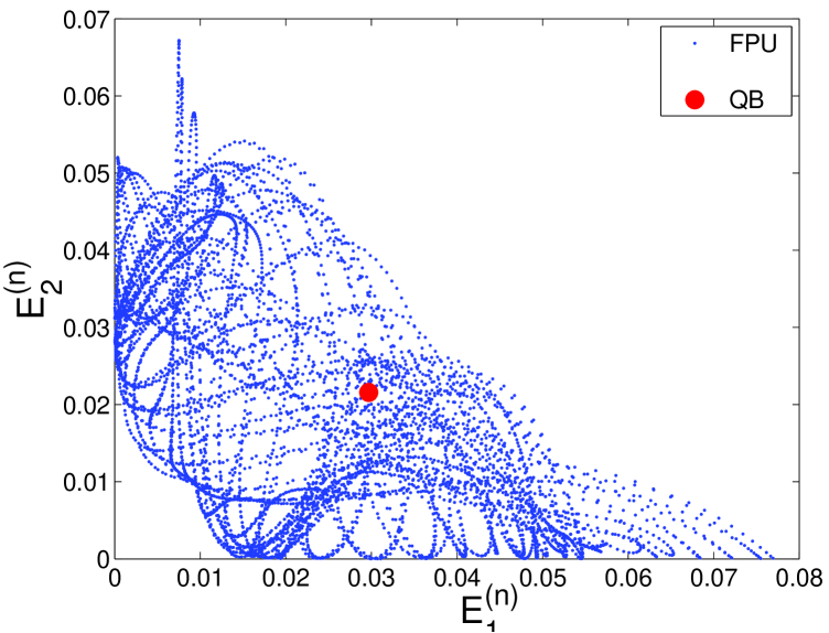
Figure 10: Map of the mode energies $E_{1}$ and $E_{2}$ on the FPU trajectory after consecutive periods of the corresponding $q$-breather for $N=32$, $\alpha=0.25$ and $q_{0}=1$. The thick dot is the results for the QB orbit.

In Fig.10 we plot the mode energies $E_{1}$ and $E_{2}$ during integration of the FPU trajectory for $\alpha=0.25$ and $q_{0}=1$ after consecutive periods of the $q$-breather solution. The regular pattern indicates regular motion, and the thick dot, which corresponds to the $q$-breather solution itself, resides inside the quasiperiodic cloud of the FPU trajectory, indicating once more that the FPU trajectory is a perturbation of the $q$-breather and evolves around the QB in phase space. Zooming the time dependence of the mode energies for the FPU trajectories on time scales comparable to the QB period shows very similar nearly periodic fluctuations as in Fig.5 which are generated by the QB period. Using the linearized phase space flow around a QB we can estimate an effective recurrence time, which for the original FPU case is two times smaller than the recurrence time for the FPU trajectory. We tracked the change of the recurrence time with increasing $\Delta$. When coming closer to the FPU trajectory, simply every second recurrence as observed for small deviations from the QB is suppressed, leaving us with the FPU recurrence time. That effect may be due to additional nonlinear contributions to the phase space flow around a QB.

Finally we note that extremely long computations of the FPU trajectory have been reported recently [27]. The trajectory localizes in $q$-space (and thus stays close to a $q$-breather) for times up to $10^{10}$. Only after that a mixing of mode energies is observed, possibly due to Arnold diffusion. Notably that critical time has been estimated by numerical scaling analysis for shorter transition times [12].

7 Towards transient processes and thermal equilibrium

Once the existence and stability of QBs as exact solutions are established, it is interesting to analyze the contribution of these trajectories to the dynamics of transient processes and thermal equilibrium. It is well-known, that in states, corresponding to energy equipartition between degrees of freedom (or thermal equilibrium) energy distribution demonstrates strong statistical properties, with no energy concentrations on average in some subparts of phase space. This circumstance, however, does not forbid existence of finite-time energy localizations whose lifetime may substantially exceed the characteristic period of plane waves. We recall the studies of discrete breather contributions to the dynamics of nonlinear lattices in thermal equilibrium and transient processes [34].

Here we present results of numerical simulations of the $\beta$-FPU chain ($N=100$, fixed boundary conditions) with two types of initial conditions: (i) all energy is located in a single mode $E_{tot}=E_{3}=1.58,E_{q\neq 3}=0$, (ii) all energy is randomly distributed among all modes: $Q_{q}(0)=\xi_{k}/\omega_{q},\ \dot{Q}_{q}(0)=\eta_{k}$, where $\xi_{k},\eta_{k}$ are random numbers, uniformly distributed in $[-c,c]$, $c$ taken to ensure $E_{tot}/N=0.2$.

In the first case we take three values of $\beta=0.6,1.25,5.0$, for which energy delocalizes and essentially redistributes among the degrees of freedom after some transition time $T_{tr}$ (Fig.11).

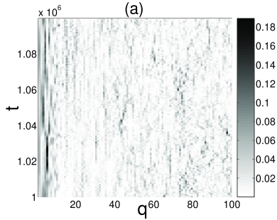
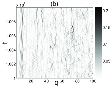
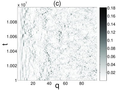
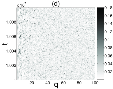
Figure 11: Space-time plots of mode energies $E_{q}$ evolving from the initial localization in the third mode for $N=100,E_{3}(0)=1.58$ and (a) $\beta=0.6,T_{tr}=10^{6}$, (b) $\beta=0.6,T_{tr}=10^{7}$, (c) $\beta=1.25,T_{tr}=10^{7}$, (d) $\beta=5.0,T_{tr}=10^{7}$.

We note that with the chosen values of $q_{0},E_{0},N$ our previous results suggest that the QB becomes unstable at $\beta\approx 0.01$ and delocalizes at $\beta\approx 1.6$. The figures show a time window width $10^{5}$ which is much larger than the largest QB periods which are of the order of 400.

We observe that stochastic motion and energy flow to higher modes lead the system into a possibly long transient regime, in which QB-like objects (finite-lifetime single-mode excitations) are observed for all $q$ (Fig.11(a,b), note that at different $T_{tr}$ qualitatively the same picture is observed). These objects survive for up to a hundred periods of phonon band oscillations. Since the smallest chosen values for $\beta$ exceed the QB instability threshold value, we conclude that the QB instability is of local character in $q$-space and does not carry a perturbed trajectory far away. When $\beta$ is increased, the lifetime of higher frequency QBs drops down and they disappear in the high- and middle-frequency regions (Fig.11(c), $\beta=1.25$), and then remain observable only in the few lowest modes (Fig.11(d), $\beta=5.0$). Note that for these values of $\beta$ we already exceed the delocalization threshold estimate for QBs. The observation of surviving low-$q$ QB-like structures suggests that the energy flow between low and high $q$ modes is sufficiently weak, so that some excess of energy is transferred into the large $q$ domain, allowing for long-time energy localization in the low $q$ domain.

Similar effects can be observed for the second type of initial conditions (Fig.12) which mimics thermal equilibrium.

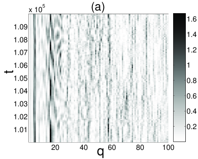
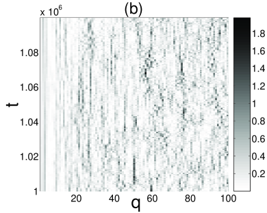
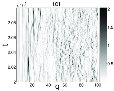
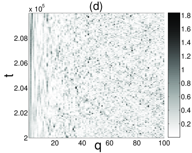
Figure 12: Space-time plots of mode energies $E_{q}$ evolving from random initial conditions for $N=100,E_{tot}/N=0.2$ and (a) $\beta=0.05,T_{tr}=10^{5}$, (b) $\beta=0.05,T_{tr}=10^{6}$, (c) $\beta=0.1,T_{tr}=2\cdot 10^{5}$, (d) $\beta=0.4,T_{tr}=2\cdot 10^{5}$.

At low $\beta$ QBs can be observed in the whole phonon band frequency domain (Fig.12(a,b), $\beta=0.05$). As $\beta$ is increased, high- and medium-frequency QBs disappear (Fig.12(c,d), $\beta=0.1,0.4$). Note, that by rescaling coordinates and momenta (and, hence, energies) the set of total energies and nonlinear coupling strengths for both types of initial conditions practically coincide, so one may directly compare all subfigures from Fig.11 and Fig.12.

8 Conclusion

We report on the existence of $q$-breathers as exact time-periodic low-frequency solutions in the nonlinear FPU system. These solutions are exponentially localized in the $q$-space of the normal modes and preserve stability for small enough nonlinearity. They continue from their trivial counterparts for zero nonlinearity at finite energy. The stability threshold of QB solutions coincides with the weak chaos threshold in [8]. The delocalization threshold estimate of QBs shows identical scaling properties as the estimate of equipartition from second order nonlinear resonance overlap [9]. Persistence of exact stable QB modes is shown to be related to the FPU observation. The FPU trajectories computed 50 years ago are perturbations of the exact QB orbits. Remarkably, localization in $q$-space persists even for parameters when the QBs turn unstable. The QB concept - tracing time-periodic and $q$-space localized orbits together with their stability and degree of localization - allows to explain quantitatively and semiquantitatively many aspects of the 50 year old FPU problem. Moreover we show that dynamical localization in $q$-space persists for transient processes and thermal equilibrium remarkably well. Note that for certain cases specific symmetries allow to obtain $q$-breathers with compact localization [28, 35], where they have been interpreted as anharmonic plane wave solutions.

The concept of QBs and their impact on the evolution of excitations in the FPU system is expected to apply far beyond the stability threshold of the QB solutions reported in the present work. Generalizations to higher dimensional lattices and other Hamiltonians are straightforward, due to the weak constraint imposed by the nonresonance condition needed for continuation. QBs can be also expected to contribute to peculiar dynamical features of nonlinear lattices in thermal equilibrium, e.g. the anomalous heat conductivity in FPU lattices [3].

A quantization of QBs will lead straightforwardly to quantum QBs, which will not differ much from their classical counterparts, due to the absence of discrete symmetries which may lead to tunneling effects. Thus a quantum QB state will be localized in $q$-space pretty much as a classical QB, allowing for ballistic-type excitations in the low-$q$ domain.

Finally we remark that the QB concept is not even constrained to an underlying lattice in real space. What we need in order to construct a QB is a discrete spectrum of mode energies, and nonlinearity which induces mode-mode interactions. Thus QBs can be constructed in various nonlinear field equations on a finite spatial domain as well, since one again obtains in the limit of small amplitudes a discrete mode spectrum, with the only difference to a finite lattice that the number of modes is infinite.


Acknowledgements

We thank T. Bountis, S. Denisov, F. Izrailev, Yu. Kosevich, A. J. Lichtenberg, P. Maniadis, V. Shalfeev and W. Zakrzewski for stimulating discussions. M.I. and O.K. appreciate the warm hospitality of the Max Planck Institute for the Physics of Complex Systems. M.I. also acknowledges support of the ”Dynasty” foundation.

Appendix A QB localization in the $\alpha$-FPU model

First, we note, that (18) and (19) are true for $k=1$, according to (17). Further, we assume it is true for $k=1,\dots,n-1$ and prove, that it is then true for $k=n$ as well.

Equation (16) for the order $n-1$ can be written as

$$\ddot{Q}^{(n-1)}_{q}+\omega_{q}^{2}Q^{(n-1)}_{q}=-\omega_{q}\mspace{-18.0mu}\sum_{\begin{subarray}{c}n_{1,2}=1\\ n_{1}+n_{2}=n\end{subarray}}^{n-1}\sum_{l,m=1}^{N}\omega_{l}\omega_{m}B_{qlm}Q^{(n_{1}-1)}_{l}Q^{(n_{2}-1)}_{m}$$ (32)

Consider, for which mode numbers $q$ the right-hand part in (32) is non-zero. As $n_{1,2}<n$, we obtain from (18a) $Q^{(n_{1}-1)}_{l}\neq 0$ for $l=q_{0},2q_{0},\dots,n_{1}q_{0}$ only, and $Q^{(n_{2}-1)}_{m}\neq 0$ for $m=q_{0},2q_{0},\dots,n_{2}q_{0}$ only. According to the definition of $B_{qlm}$ (6) and taking into account that $nq_{0}\leq N$, we obtain $B_{qlm}\neq 0$ for $q=l+m$ and $q=|l-m|$. Then, the maximal mode number $q$, for which the right-hand part in (32) is non-zero, equals $q_{max}=n_{1}q_{0}+n_{2}q_{0}=nq_{0}$. This is equivalent to (18a) at $k=n$, which concludes the induction for (18).

To prove (19), we write down (32) for $q=nq_{0}$:

$$\ddot{Q}^{(n-1)}_{nq_{0}}+\omega_{nq_{0}}^{2}Q^{(n-1)}_{nq_{0}}=-\omega_{nq_{0}}\mspace{-18.0mu}\sum_{\begin{subarray}{c}n_{1,2}=1\\ n_{1}+n_{2}=n\end{subarray}}^{n-1}\mspace{-18.0mu}\omega_{n_{1}}\omega_{n_{2}}Q^{(n_{1}-1)}_{n_{1}q_{0}}Q^{(n_{2}-1)}_{n_{2}q_{0}}$$ (33a)

Here we have taken into account, that the only non-zero term of the sum over $$l m l=n_{1}q_{0} m=n_{2}q_{0} B_{nq_{0},n_{1}q_{0},n_{2}q_{0}}=1$$ and corresponds to , , and that .

As $n_{1,2}<n$, the variables $Q^{(n_{1}-1)}_{n_{1}}$ and $Q^{(n_{2}-1)}_{n_{2}}$ are expressed via (19a). Then (33a) becomes a forced harmonic oscillator equation with a set of cosinusoidal harmonics in the right-hand part:

$$\ddot{Q}^{(n-1)}_{nq_{0}}+\omega_{nq_{0}}^{2}Q^{(n-1)}_{nq_{0}}=\sum_{m=0}^{n}C_{m}\cos m\omega_{q_{0}}t$$ (33b)

where $C_{m}$ are amplitudes of the harmonics.

Omitting the free-motion part of the solution, we write down the expression for the forced oscillations of $Q^{(n-1)}_{nq_{0}}$:

$$Q^{(n-1)}_{nq_{0}}=\sum_{m=0}^{n}\frac{C_{m}}{\omega_{nq_{0}}^{2}-m^{2}\omega_{q_{0}}^{2}}\cos m\omega_{q_{0}}t$$ (34)

Note, that the resonance denominator in (34) is minimal at $m=n$. In other words, driving frequency $n\omega_{q_{0}}$ is the closest to the resonance among all the harmonics. Expanding the sine function in (8) into a Taylor series as $\sin x=x-x^{3}/6+O(x^{5})$, we approximate the mode frequencies as

$$\omega_{q}=4\left((q\varkappa)^{2}-\frac{1}{3}(q\varkappa)^{4}+O\left((q\varkappa)^{6}\right)\right)\quad\mbox{where}\quad\varkappa=\frac{\pi}{2(N+1)}\to 0$$ (35)

The mentioned minimal denominator is then expressed at $nq_{0}/N\to 0$ as follows:

$$\omega_{nq_{0}}^{2}-n^{2}\omega_{q_{0}}^{2}=-\frac{1}{12}n^{2}(n^{2}-1)\omega_{q_{0}}^{4}+O\left(\left(\frac{nq_{0}}{N}\right)^{6}\right)$$ (36)

At the same time the relation of this denominator to any other one with $m\neq n$ is estimated as

$$\frac{\omega_{nq_{0}}^{2}-n^{2}\omega_{q_{0}}^{2}}{\omega_{nq_{0}}^{2}-m^{2}\omega_{q_{0}}^{2}}=O\left(\left(\frac{nq_{0}}{N}\right)^{2}\right)\mbox{,}\quad m\neq n$$ (37)

It means, that the harmonic $m=n$ dominates in the solution (34), while all the other harmonics are small values of the order $O\left((nq_{0}/N)^{2}\right)$ with respect to this dominating one.

Thus, (34) can be rewritten as

$$Q^{(n-1)}_{nq_{0}}=\frac{12\,C_{n}}{n^{2}(n^{2}-1)\omega_{q_{0}}^{4}}\cos n\omega_{q_{0}}t\left(1+O\left(\left(\frac{nq_{0}}{N}\right)^{2}\right)\right)$$ (38)

Inserting (19a) (valid as $n_{1,2}<n$) into (33a), we obtain the following expression for the $n$th harmonic amplitude $C_{n}$ in (33b):

$$C_{n}=-\omega_{nq_{0}}\mspace{-18.0mu}\sum_{\begin{subarray}{c}n_{1,2}=1\\ n_{1}+n_{2}=n\end{subarray}}^{n-1}\mspace{-18.0mu}\omega_{n_{1}}\omega_{n_{2}}\frac{1}{2}A_{n_{1}q_{0}}A_{n_{2}q_{0}}\cdot\left(1+O\left(\left(\frac{nq_{0}}{N}\right)^{2}\right)\right)$$ (39)

Inserting (39) into (38) and taking into account (35), we arrive at

$$Q^{(n-1)}_{nq_{0}}=A_{nq_{0}}\left(\cos n\omega_{q_{0}}t+O\left(\left(\frac{nq_{0}}{N}\right)^{2}\right)\right)$$ (40)

where

$$A_{nq_{0}}=\frac{6}{n^{2}(n^{2}-1)\omega_{q_{0}}}\sum_{\begin{subarray}{c}n_{1,2}=1\\ n_{1}+n_{2}=n\end{subarray}}^{n-1}\mspace{-18.0mu}n_{1}n_{2}A_{n_{1}q_{0}}A_{n_{2}q_{0}}$$ (41)

Expressing $A_{n_{1}q_{0}}$ and $A_{n_{2}q_{0}}$ via (19b) (valid because $n_{1,2}<n$) and taking into account that

$$\sum_{\begin{subarray}{c}n_{1,2}=1\\ n_{1}+n_{2}=n\end{subarray}}^{n-1}n_{1}n_{2}\equiv\frac{1}{6}n^{2}(n^{2}-1)\mbox{,}$$

we obtain

$$A_{nq_{0}}=\frac{A_{q_{0}}^{n}}{\omega_{q_{0}}^{n-1}}\mbox{.}$$ (42)

Equations (40) and (42) coincide with (19a,b) at $k=n$, thus concluding the induction.

Appendix B QB Stability in the $\beta$-FPU model

Making a replacement (23) in the equations of motion (5) and keeping only linear in $\xi_{q}$ terms we obtain an equation describing the dynamics of infinitesimal deviations from the QB orbit:

$$\ddot{\xi}_{q}+\omega_{q}^{2}\xi_{q}=-3\rho{\hat{Q}_{q_{0}}}^{2}(t)\omega_{q_{0}}^{2}\sum_{r=1}^{N}b_{qr}\xi_{r}+O(\rho^{2},\xi_{l})\mbox{,}$$ (43)

where $b_{qr}=\omega_{q}\omega_{r}C_{q_{0},q_{0},q,r}$, and $O(\rho^{2},\xi_{l})$ denotes a linear form of $\{\xi_{l}\}$ with small coefficients of the order $O(\rho^{2})$.

Inserting here $\hat{Q}_{q_{0}}(t)$ from (27), we obtain the following Mathieu equation:

$$\ddot{\xi}_{q}+\omega_{q}^{2}\xi_{q}=-h(1+\cos\Omega t)\sum_{r=1}^{N}b_{qr}\xi_{r}+O(h^{2},\xi_{l})\mbox{,}$$ (44)

where $h=3\rho E_{q_{0}}$, $\Omega=2\hat{\omega}$.

In the vector-matrix form it can be rewritten as follows:

$$\ddot{\boldsymbol{\xi}}+\boldsymbol{A}\boldsymbol{\xi}+h(1+\cos\Omega t)\boldsymbol{B}\boldsymbol{\xi}=O(h^{2}\boldsymbol{\xi}),$$ (45)

where $\boldsymbol{\xi}=(\xi_{q})$ is a vector, $\boldsymbol{A}=(a_{qr})$ is a diagonal matrix with elements $a_{qr}=\delta_{qr}\omega_{q}^{2}$, $\boldsymbol{B}=(b_{qr})$ is the coupling matrix.

Further, we analyze parametric resonance in the equation (45), treating $h$ and $\Omega$ as independent parameters, and then recall their dependence.

In the limit $h\to 0$ the equilibrium point $\boldsymbol{\xi}=0$ is strongly stable for all values of $\Omega$ except for a finite number of values $\Omega_{nkl}$ which satisfy

$$\omega_{k}+\omega_{l}=n\Omega_{nkl}$$ (46)

where $n$ is a natural number, and the modes $k$ and $l$ belong to the same connected component of the coupling graph whose connectivity is defined by the matrix $\boldsymbol{B}$. Strong stability implies that this point is also stable for all hamiltonian systems close enough to the considered one.

Each point $(\Omega_{nkl},0)$ on the plane of parameters $(\Omega,h)$ is associated with a zone of parametric resonance. Restricting ourselves to the case of primary resonance, which necessarily requires $n=1$ in (46), we specify the frequency $\Omega$ as

$$\Omega=(\omega_{k}+\omega_{l})(1+\delta)\mbox{,}$$ (47)

where the detuning parameter $\delta$ is assumed to be the order $\delta=O(h)$. We seek for a solution to (45) in the form

$$\boldsymbol{\xi}=\sum_{m=-\infty}^{+\infty}\boldsymbol{f}^{m}e^{(i\tilde{\omega}_{1}+z+im\Omega)t}+\mbox{c.c.}$$ (48)

where $\tilde{\omega}_{1}=\omega_{k}(1+\delta)$, $\boldsymbol{f}^{m}=(f_{q}^{m})$ are unknown complex vector amplitudes, and $z$ is a small unknown complex number. We make an assumption $z=O(h)$ which is confirmed further in the course of the calculation.

Inserting (48) into (45) we obtain a system of algebraic equations for the amplitudes $f_{q}^{m}$:

$$\left[2iz(\tilde{\omega}_{1}+m\Omega)-(\tilde{\omega}_{1}+m\Omega)^{2}+\omega_{q}^{2}\right]f_{q}^{m}+\\ +(h\boldsymbol{B}\boldsymbol{f}^{m})_{q}+\left(\frac{h}{2}\boldsymbol{B}(\boldsymbol{f}^{m+1}+\boldsymbol{f}^{m-1})\right)_{q}=O(h^{2}|\boldsymbol{\xi}|)$$ (49)

Note, that if the coefficient in square brackets in (49) is not a small value of the order $O(h)$, then the corresponding amplitude $f_{q}^{m}$ is itself a small value of the order $O(h|\boldsymbol{\xi}|)$. Let us find out, for which values of the indices $m$ and $q$ the mentioned coefficient is small. As we assume $z=O(h)$, the difference $-(\tilde{\omega}_{1}+m\Omega)^{2}+\omega_{q}^{2}$ needs to be a small value. It will be so, if the absolute value $|\tilde{\omega}_{1}+m\Omega|$ is close to one of the eigenfrequencies $\omega_{q}$. According to the definition of $\tilde{\omega}_{1}$ and the expression for $\Omega$ (47), this implies $|(m+1)\omega_{k}+m\omega_{l}|=\omega_{q}$. Generically, due to the incommensurate eigenfrequencies spectrum, this condition is only fulfilled for $m=0$, $q=k$ or $m=-1$, $q=l$.

It follows, that all amplitudes $f_{q}^{m}$ except for $f^{0}_{k}$ and $f^{-1}_{l}$ are small values of the order $O(h|\boldsymbol{\xi}|)$. Then we are able to write down a closed system for $f^{0}_{k}$ and $f^{-1}_{l}$ accurate to $O(h^{2}|\boldsymbol{\xi}|)$:

$$(2iz\tilde{\omega}_{1}+2\omega_{k}^{2}(h-\delta))f^{0}_{k}+\frac{h}{2}b_{kl}f^{-1}_{l} =O(h^{2}|\boldsymbol{\xi}|)$$ (50a)

$$\frac{h}{2}b_{lk}f^{0}_{k}+(-2iz\tilde{\omega}_{2}+2\omega_{l}^{2}(h-\delta))f^{-1}_{l} =O(h^{2}|\boldsymbol{\xi}|)$$ (50b)

where $\tilde{\omega}_{2}=\Omega-\tilde{\omega}_{1}=\omega_{l}(1+\delta)$. Note, that for a primary resonance the coupling coefficient $b_{kl}$ must be non-zero, which means that the mode oscillators $k$ and $l$ are directly coupled.

A nontrivial solution to this system exists if the determinant of the left-hand part (with an error $O(h^{2})$ allowed for in each element) equals zero. From this condition we derive

$$z_{1,2}=-i\frac{(h-\delta)(\omega_{l}-\omega_{k})}{2}\pm\frac{1}{2}\sqrt{\frac{h^{2}}{4}\omega_{k}\omega_{l}-(h-\delta)^{2}(\omega_{k}+\omega_{l})^{2}+O(h^{3})}+O(h^{2})$$ (51)

In the initial problem both $h$ and $\Omega$ depend on the nonlinearity magnitude $\beta E_{q_{0}}$. This dependence defines a line starting from the point $(2\omega_{m_{0}},0)$ on the $(\Omega,h)$ plane. The intersections of this line with the resonance zones are the regions of the QB orbit instability.

The nearest primary resonance corresponds to $k=m_{0}-1$, $l=m_{0}+1$, $n=1$. In this case we can derive a simpler expression for $z_{1,2}$ in the vicinity of the bifurcation point (near the edge of the resonance zone) if we let $N\to\infty$ at the same time assuming $q_{0}/(N+1)=const$ which means $\omega_{q_{0}}=const$.

From (35) we obtain

$$\omega_{q_{0}+1}-\omega_{q_{0}-1} =2\cos q_{0}\varkappa\cdot(1+O(\varkappa^{2}))$$ (52a)

$$\omega_{q_{0}+1}\omega_{q_{0}-1} =\omega_{q_{0}}^{2}\cdot(1+O(\varkappa^{2}))$$ (52b)

$$\omega_{q_{0}+1}+\omega_{q_{0}-1} =2\omega_{q_{0}}\cdot(1+O(\varkappa^{2}))$$ (52c)

Then we express $\delta$ from (47):

$$\delta=\frac{\Omega}{\omega_{q_{0}+1}+\omega_{q_{0}-1}}-1=\frac{3}{4}h+\frac{1}{2}\varkappa^{2}+O(\varkappa^{4})$$ (53)

Inserting (52a-c) and (53) into (51) and taking into account that if we are close to the bifurcation point (the expression under the square root in (51) is close to zero) then $h=O(\varkappa^{2})$, we find

$$z_{1,2}=\pm\frac{1}{2}\omega_{q_{0}}\varkappa^{2}\sqrt{R-1+O(\varkappa^{2})}+i\cdot O(\varkappa^{3})$$ (54)

where $R=h/\varkappa^{2}=6\beta E_{q_{0}}(N+1)/\pi^{2}$.

According to (48), the absolute values of the Floquet multipliers involved in the resonance are calculated as

$$|\lambda_{j_{1}j_{2}}|=\exp(\frac{2\pi\mbox{Re}z_{1,2}}{\Omega})\mbox{,}$$ (55)

which finally leads to (30).

References

- [1] E. Fermi, J. Pasta, and S. Ulam, Los Alamos Report LA-1940, (1955); also in: Collected Papers of Enrico Fermi, ed. E. Segre, Vol. II (University of Chicago Press, 1965) p.978; Many-Body Problems, ed. D. C. Mattis (World Scientific, Singapore, 1993).
- [2] J. Ford, Phys. Rep. 213, 271 (1992).
- [3] CHAOS 15 Nr.1 (2005), Focus Issue The Fermi-Pasta-Ulam problem - The first fifty years, Eds. D. K. Campbell, P. Rosenau and G. M. Zaslavsky.
- [4] G. P. Berman and F. M. Izrailev, CHAOS 15, 015104 (2005).
- [5] N. J. Zabusky and M. D. Kruskal, Phys. Rev. Lett. 15, 240-243 (1965).
- [6] F. M. Izrailev and B. V. Chirikov, Institute of Nuclear Physics, Novosibirsk, USSR, 1965 (in Russian); Dokl. Akad. Nauk SSSR 166, 57 (1966) [Soviet. Phys. Dokl. 11, 30 (1966)].
- [7] B. V. Chirikov, Atomnaya Energia 6, 630 (1959) [Engl. Transl. J.Nucl. Energy Part C: Plasma Phys. 1, 253 (1960)].
- [8] J. De Luca, A. J. Lichtenberg, and M. A. Lieberman, CHAOS, 5, 283 (1995).
- [9] D.L. Shepelyansky, Low-energy chaos in the Fermi-Pasta-Ulam problem, Nonlinearity 10, 1331 (1997).
- [10] P. Bocchierri, A. Scotti, B. Bearzi, and A. Loigner, Phys. Rev. A 2, 2013 (1970); L. Galgani and A. Scotti, Phys. Rev. Lett. 28, 1173 (1972); A. Patrascioiu, Phys. Rev. Lett. 50, 1879 (1983).
- [11] H. Kantz, Physica D 39, 322 (1989); H. Kantz, R. Livi and S. Ruffo, J. Stat. Phys. 76, 627 (1994).
- [12] L. Casetti, M. Cerruti-Sola, M. Pettini and E. G. D. Cohen, Phys. Rev. E 55, 6566 (1997).
- [13] P. Bocchieri, A. Scotti, B. Bearzi and A. Loinger, Phys. Rev. A 2, 2013 (1970).
- [14] S. Flach, M. V. Ivanchenko and O. I. Kanakov, Phys. Rev. Lett. 95, 064102 (2005).
- [15] S. Flach and C. R. Willis, Phys. Rep. 295, 181 (1998) and references therein.
- [16] A. J. Sievers and J. B. Page, in: Dynamical properties of solids VII phonon physics the cutting edge, Elsevier, Amsterdam (1995); S. Aubry, Physica D 103, 201 (1997); Energy Localisation and Transfer, Eds. T. Dauxois, A. Litvak-Hinenzon, R. MacKay and A. Spanoudaki, World Scientific (2004); D. K. Campbell, S. Flach and Yu. S. Kivshar, Physics Today, p.43, January 2004.
- [17] S. Flach and A. Gorbach, CHAOS 15, 015112 (2005).
- [18] R. S. MacKay and S. Aubry, Nonlinearity 7, 1623 (1994).
- [19] R. Livi, M. Spicci and R. S. MacKay, Nonlinearity 10, 1421 (1997).
- [20] S. Aubry, Ann. Inst. H. Poincare, Phys. Theor. 68, 381 (1998); S. Aubry, G. Kopidakis and V. Kadelburg, Discrete and Continuous Dynamical Systems B 1, 271 (2001).
- [21] G. James, C. R. Acad. Sci. Paris 332, 581 (2001).
- [22] S. Flach, Phys. Rev. E 50, 3134 (1994); J. L. Marin and S. Aubry, Nonlinearity 9, 1501 (1996); B. Dey, M. Eleftheriou, S. Flach and G. Tsironis, Phys. Rev. E 65, 017601 (2002); P. Rosenau and S. Schochet, Phys. Rev. Lett. 94, 045503 (2005).
- [23] S. Flach, Phys. Rev. E 58, R4116 (1998).
- [24] M. A. Lyapunov. Probleme Generale de la Stabilite du Mouvement, Princeton Univ. Press, 375-392 (1949); J. Horn, Z. Math. Phys. 48, 400 (1903).
- [25] A. Zygmund, Trigonometric Series, Cambridge University Press, Cambridge, England (1968).
- [26] Note that we do not demand specific symmetries leading to low-dimensional invariant manifolds in phase space, in contrast to the discussion in [28, 35]. Consequently, our QB solutions do not have to be embedded in such subspaces.
- [27] A. Giorgilli, S. Paleari and T. Penati, Discr. and Contin. Dyn. Syst. B 5, 1 (2005).
- [28] R. L. Bivins, N. Metropolis, and J. R. Pasta, J. Comput. Phys. 12, 65 (1973); B. Rink, Physica D 175, 31 (2003) and references therein.
- [29] L. Berchialla, A. Giorgilli and S. Paleari, Phys. Lett. A 321, 167 (2004).
- [30] J. DeLuca, A. J. Lichtenberg and S. Ruffo, Phys. Rev. E 51, 2877 (1995).
- [31] The subsequent bifurcations of the same type are associated with next primary resonances of the type , , , . The corresponding bifurcation points are located at . Note, that higher-order resonances at certain values of and may result in appearance of narrow instability regions within the region .
- [32] C. F. Driscoll and T. M. O’Neil, Phys. Rev. Lett. 37, 69 (1976).
- [33] J. DeLuca, A. J. Lichtenberg and S. Ruffo, Phys. Rev. E 60, 3781 (1999).
- [34] I. Daumont, T. Dauxois, M. Peyrard, Nonlinearity 10, 617 (1997); M. Peyrard, Physica D, 119, 184 (1998); T. Cretegny, T. Dauxois, S. Ruffo and A. Torcini, Physica D 121, 109 (1998); M. Johansson, A. M. Morgante, S. Aubry and G. Kopidakis, Eur. Phys. J. B 29, 279 (2002); B. Rumpf and A. C. Newell, Phys. Rev. Lett. 87, 054102 (2001); B. Rumpf and A. C. Newell, Physica D 184, 162 (2003); G. P. Tsironis and S. Aubry, Phys. Rev. Lett. 77 5225 (1996); A. Bikaki et al., Phys. Rev. E 59, 1234 (1999); R. Reigada, A. Sarmiento and K. Lindenberg, Phys. Rev. E 64 066608 (2001); S. Flach and G. Mutschke, Phys. Rev. E 49, 5018 (1994); M. Eleftheriou, S. Flach and G. P. Tsironis, Physica D 186, 20 (2003); M. V. Ivanchenko, O. I. Kanakov, V. D. Shalfeev and S. Flach, Physica D 198, 120 (2004); M. Eleftheriou and S. Flach, Physica D 202, 142 (2005).
- [35] N. Budinsky and T. Bountis, Physica D 8, 445 (1983); Y. A. Kosevich, Phys. Rev. Lett. 71, 2058 (1993); S. Flach, Physica D 91, 223 (1996); P. Poggi and S. Ruffo, Physica D 103, 251 (1997).