Coarse-graining of cellular automata, emergence, and the predictability of complex systems

Abstract

We study the predictability of emergent phenomena in complex systems. Using nearest neighbor, one-dimensional Cellular Automata (CA) as an example, we show how to construct local coarse-grained descriptions of CA in all classes of Wolfram’s classification. The resulting coarse-grained CA that we construct are capable of emulating the large-scale behavior of the original systems without accounting for small-scale details. Several CA that can be coarse-grained by this construction are known to be universal Turing machines; they can emulate any CA or other computing devices and are therefore undecidable. We thus show that because in practice one only seeks coarse-grained information, complex physical systems can be predictable and even decidable at some level of description. The renormalization group flows that we construct induce a hierarchy of CA rules. This hierarchy agrees well with apparent rule complexity and is therefore a good candidate for a complexity measure and a classification method. Finally we argue that the large scale dynamics of CA can be very simple, at least when measured by the Kolmogorov complexity of the large scale update rule, and moreover exhibits a novel scaling law. We show that because of this large-scale simplicity, the probability of finding a coarse-grained description of CA approaches unity as one goes to increasingly coarser scales. We interpret this large scale simplicity as a pattern formation mechanism in which large scale patterns are forced upon the system by the simplicity of the rules that govern the large scale dynamics.

I Introduction

The scope of the growing field of “complexity science” (or “complex systems”) includes a broad variety of problems belonging to different scientific areas. Examples for “complex systems” can be found in physics, biology, computer science, ecology, economy, sociology and other fields. A recurring theme in most of what is classified as “complex systems” is that of emergence. Emergent properties are those which arise spontaneously from the collective dynamics of a large assemblage of interacting parts. A basic question one asks in this context is how to derive and predict the emergent properties from the behavior of the individual parts. In other words, the central issue is how to extract large-scale, global properties from the underlying or microscopic degrees of freedom.

In the physical sciences, there are many examples of emergent phenomena where it is indeed possible to relate the microscopic and macroscopic worlds. Physical systems are typically described in terms of equations of motion of a huge number of microscopic degrees of freedom (e.g. atoms). The microscopic dynamics is often erratic and complex, yet in many cases it gives rise to patterns with characteristic length and time scales much larger than the microscopic ones (e.g. the pressure and temperature of a gas). These large scale patterns often posses the interesting, physically relevant properties of the system and one would like to model them or simulate their behavior. An important problem in physics is therefore to understand and predict the emergence of large scale behavior in a system, starting from its microscopic description. This problem is a fundamental one because most physical systems contain too many parts to be simulated directly and would become intractable without a large reduction in the number of degrees of freedom. A useful way to address this issue is to construct coarse-grained models, which treat the dynamics of the large scale patterns. The derivation of coarse-grained models from the microscopic dynamics is far from trivial. In most cases it is done in a phenomenological manner by introducing various (often uncontrolled) approximations.

The problem of predicting emergent properties is most severe in systems which are modelled or described by undecidable mathematical algorithmsWolfram (1984a); Moore (1990). For such systems there exists no computationally efficient way of predicting their long time evolution. In order to know the system’s state after (e.g.) one million time steps one must evolve the system a million time steps or perform a computation of equivalent complexity. Wolfram has termed such systems computationally irreducible and suggested that their existence in nature is at the root of our apparent inability to model and understand complex systems Wolfram (1984a, 1985, 2002); Ilachinski (2001). It is tempting to conclude from this that the enterprise of physics itself is doomed from the outset; rather than attempting to construct solvable mathematical models of physical processes, computational models should be built, explored and empirically analyzed. This argument, however, assumes that infinite precision is required for the prediction of future evolution. As we mentioned above, usually coarse-grained or even statistical information is sufficient. An interesting question that arises is therefore: is it possible to derive coarse-grained models of undecidable systems and can these coarse-grained models be decidable and predictable?

In this work we address the emergence of large scale patterns in complex systems and the associated predictability problems by studying Cellular-Automata (CA). CA are spatially and temporally discrete dynamical systems composed of a lattice of cells. They were originally introduced by von Neumann and Ulam von Neumann (1966) in the 1940’s as a possible way of simulating self-reproduction in biological systems. Since then, CA have attracted a great deal of interest in physics Wolfram (1983); phy ; Ilachinski (2001); Wolfram (1994) because they capture two basic ingredients of many physical systems: 1) they evolve according to a local uniform rule. 2) CA can exhibit rich behavior even with very simple update rules. For similar and other reasons, CA have also attracted attention in computer science Mitchel (1998); Sarkar (2000), biology Ermentrout and Edelstein-Keshet (1993), material science Raabe (2002) and many other fields. For a review on the literature on CA see Refs. Ilachinski, 2001; Wolfram, 1994, 2002.

The simple construction of CA makes them accessible to computational theoretic research methods. Using these methods it is sometimes possible to quantify the complexity of CA rules according to the types of computations they are capable of performing. This together with the fact that CA are caricatures of physical systems has led many authors to use them as a conceptual vehicle for studying complexity and pattern formation. In this work we adopt this approach and study the predictability of emergent patterns in complex systems by attempting to systematically coarse-grain CA. A brief preliminary report of our project can be found in Ref. Israeli and Goldenfeld, 2004.

There is no unique way to define coarse-graining, but here we will mean that our information about the CA is locally coarse-grained in the sense of being stroboscopic in time, but that nearby cells are grouped into a supercell according to some specified rule (as is frequently done in statistical physics). Below we shall frequently drop the qualifier ”local” whenever there is no cause for confusion. A system which can be coarse-grained is compact-able since it is possible to calculate its future time evolution (or some coarse aspects of it) using a more compact algorithm than its native description. Note that our use of the term compact-able refers to the phase space reduction associated with coarse-graining, and is agnostic as to whether or not the coarse-grained system is decidable or undecidable. Accordingly, we define predictable to mean that a system is decidable or has a decidable coarse-graining. Thus, it is possible to calculate the future time evolution of a predictable system (or some coarse aspects of it) using an algorithm which is more compact than both the native and coarse-grained descriptions.

Our work is organized as follows. In section II we give an introduction to CA and their use in the study of complexity. In section III we present a procedure for coarse-graining CA. Section IV shows and discusses the results of applying our procedure to one dimensional CA. Most of the CA that we attempt to coarse-grain are Wolfram’s 256 elementary rules for nearest-neighbor CA. We will also consider a few other rules of special interest. In section V we consider whether the coarse-grain-ability of many CA that we found in the elementary rule family is a common property of CA. Using computational theoretic arguments we argue that the large scale behavior of local processes must be very simple. Almost all CA can therefore be coarse-grained if we go to a large enough scale. Our results are summarized and discussed in VI.

II Cellular Automata

Cellular automata are a class of homogeneous, local and fully discrete dynamical systems. A cellular automaton $A=\left(a\left(t\right),\{S_{A}\},f_{A}\right)$ is composed of a lattice $a(t)$ of cells that can each assume a value from a finite alphabet $\{S_{A}\}$. We denote individual lattice cells by $a_{\alpha}\left(t\right)$ where the indexing reflects the dimensionality and geometry of the lattice. Cell values evolve in discrete time steps according to the pre-prescribed update rule $f_{A}$. The update rule determines a cell’s new state as a function of cell values in a finite neighborhood. For example, in the case of a one dimensional, nearest-neighbor CA the update rule is a function $f_{A}:\{S_{A}\}^{3}\rightarrow\{S_{A}\}$ and $a_{n}\left(t+1\right)=f_{A}\left[a_{n-1}\left(t\right),a_{n}\left(t\right),a_{n+1}\left(t\right)\right]$. At each time step, each cell in the lattice applies the update rule and updates its state accordingly. The application of the update rule is done in parallel for all the cells and all the cells apply the same rule. We denote the application of the update rule on the entire lattice by $a\left(t+1\right)=f_{A}\cdot a\left(t\right)$.

In early work Wolfram (1984b, a, 1985, 2002), Wolfram proposed that CA can be grouped into four classes of complexity. Class 1 consists of CA whose dynamics reaches a steady state regardless of the initial conditions. Class 2 consists of CA whose long time evolution produces periodic or nested structures. CA from both of these classes are simple in the sense that their long time evolution can be deduced from running the system a small number of time steps. On the other hand, class 3 and class 4 consist of “complex” CA. Class 3 CA produce structures that seem random. Class 4 CA produce localized structures that propagate and interact in a complex way above a regular background. This classification is heuristic and the assignment of CA to the four classes is somewhat subjective. Successive works on CA attempted to improve it or to find better alternativesCulik and Yu (1988); Gutowitz (1988, 1990); Stuner (1990); Binder (1991); Braga et al. (1995); Jin and Kim (2003). To the best of our knowledge there is, to date, no universally agreed upon classification scheme of CA.

Based on numerical experiments, Wolfram hypothesized that most of class 3 and 4 CA are Computationally IrreducibleWolfram (1984b, a, 2002). Namely, the evolution of these CA cannot be predicted by a process which is drastically more efficient than themselves. In order to calculate the state of a Computationally Irreducible CA after $t$ time steps, one must run the CA for $t$ time steps or perform a computation of equivalent complexity. This definition is somewhat loose because it is not always clear how to compare computation running times and efficiency on different architectures. In addition, Wolfram recognized that even computationally irreducible systems may have some “superficial reducibility” (see page 746 in Ref. Wolfram, 2002) and can be reduced to a limited extent. The difference between “superficial” and true reducibility however is not well defined. It is nevertheless clear that the asymptotic $t\rightarrow\infty$ behavior of a Computationally Irreducible system cannot be predicted by any computation of finite size. Wolfram further argued that Computationally Irreducible systems are abundant in nature and that this fact explains our inability as physicists to deal with complex systems Wolfram (1984a, 1985, 2002); Ilachinski (2001).

It is difficult in general to tell whether a CA, behaving in an apparently complex way, is Computationally Irreducible. More concrete properties of CA which are related to Computational Irreducibility are Undecidability and Universality. Mathematical processes are said to be undecidable when there can be no algorithm that is guaranteed to predict their outcome in a finite time. Equivalently, CA are said to be undecidable when aspects of their dynamics are undecidable. Computationally Irreducible CA are therefore Undecidable and in the weak asymptotic definition that we gave above, Computational Irreducibility is equivalent to Undecidability. For lack of a better choice we adopt this asymptotic definition and in the reminder of this work we will use the two terms interchangeably.

Some CA are known to be universal Turing machinesHerken (1995) and are capable of performing all computations done by other processes. A famous two dimensional example is Conway’s game of lifeGardner (1970); several examples in one dimension are Lindgren and Nordahl Lindgren and G. (1990), Albert and Culik Albert and K. (1987) and Wolfram’s rule 110 Wolfram (2002). Universal CA are, in a sense, maximally complex because they can emulate the dynamics of all other CA. Being universal Turing machines, these CA are subject to undecidable questions regarding their dynamicsWolfram (1984b). For example whether an initial state will ever decay into a quiescent state is the CA equivalence of the undecidable halting problemHerken (1995). Universal CA are therefore Undecidable.

Wolfram’s classification of CA is topological in the sense that CA are classified according to the properties of their trajectories. A different, more ambitious, approach is to classify CA according to a parameter derived directly from their rule tables. Langton Langton (1990) suggested that CA rules can be parameterized by his $\lambda$ parameter which measures the fraction of non-quiescence rule table entries. He showed a strong correlation between the value of $\lambda$ and the complexity found in the CA trajectories. For small values of $\lambda$ one characteristically finds class 1 and 2 behavior while for $\lambda\sim 1$ a class 3 behavior is usually observed. Langton identified a narrow region of intermediate values of $\lambda$ where he found class 4 characteristic behavior. Based on these observations Langton proposed the edge of chaos hypothesisLangton (1990). This hypothesis claims that in the space of dynamical systems, interesting systems which are capable of computation are located at the boundary between simple and chaotic systems. This appealing hypothesis however was criticized in later works Mitchell et al. (1993). Recently, a different parametrization of CA rule tables was proposed by Dubacq et al. Dubacq et al. (2001). This new approach is based on the information content of the rule table as measured by its Kolmogorov Complexity. As we will show below, our results lend support to this notion and indicate that rule tables with low Kolmogorov complexity lead to simple behavior and vice versa.

In addition to attempts to find order and hierarchy in the space of CA rules, much research has been devoted to the study of CA classes with special properties. Additive CA (or linear) Robinson (1987); Barbe et al. (1995), commuting CA Voorhees (1993) and CA with certain algebraic properties Moore (1997, 1998) are a few examples. Unsurprisingly, the dynamics of CA which enjoy such special properties can in most cases be understood and predictable at some level.

In this work we will mostly be concerned with the family of one dimensional, nearest neighbor binary CA that were the subject of Wolfram’s investigations. These 256 elementary rules are among the simplest imaginable CA and thus present us with the least computational challenges when attempting to coarse-grain them. We will use Wolfram’s notationWolfram (1983) for identifying individual rules. The update function of an elementary rule is described by a rule number between 0 and 255. The eight bit binary representation of the rule number specifies the update function outcome for the eight possible three cell configurations (where “000” is the least significant and “111” is the most significant bit). CA are often conveniently visualized with different colors denoting different cell values. When dealing with binary CA we will use the convention $\square=0$, $\blacksquare=1$ and use the two notations interchangeably.

III Local coarse-graining of Cellular Automata

We now turn to study the emergence of large scale patterns in CA and the associated predictability problems by attempting to coarse-grain CA. There are many ways to define a coarse-graining of a dynamical system. In this work we define it as a (real-space) renormalization scheme where the original CA $A=\left(a\left(t\right),\{S_{A}\},f_{A}\right)$ is coarse-grained to a renormlized CA $B=\left(b\left(t\right),\{S_{B}\},f_{B}\right)$ through the lattice transformation $b_{k}=P\left(a_{N\cdot k},a_{N\cdot k+1},\dots,a_{N\cdot k+N-1}\right)$. The projection function $P:\{S_{A}\}^{N}\rightarrow\{S_{B}\}$ projects the value of a block of $N$ cells in $A$, which we term a supercell, to a single cell in $B$. By writing $P\cdot a$ we denote the block-wise application of $P$ on the entire lattice $a$. Only non-trivial cases where $P$ is irreversible are considered because we want $B$ to provide a partial account of the full dynamics of $A$.

In order for $B$ and $P$ to provide a coarse-grained emulation of $A$ they must satisfy the commutativity condition

$$P\cdot f_{A}^{T}\cdot a(0)=f_{B}\cdot P\cdot a(0)\;,$$ (1)

for every initial condition $a(0)$ of $A$. The constant $T$ in the above equation is a time scale associated with the coarse-graining. A repeated application of Eq. (1) shows that

$$P\cdot f_{A}^{T\cdot t}\cdot a(0)=f_{B}^{t}\cdot P\cdot a(0)\;,$$ (2)

for all $t$. Namely, running the original CA for $T\cdot t$ time steps and then projecting is equivalent to projecting the initial condition and then running the renormalized CA for $t$ time steps. Thus, if we are only interested in the projected information we can run the more efficient CA $B$.

Renormalization group transformations in statistical physics are usually performed with projection operators that arise from a physical intuition and understanding of the system in question. Majority rules and different types of averages are often the projection operators of choice. In this work we have the advantage that the CA we wish to coarse-grain are fully discrete systems and the number of possible projections of a supercell of size $N$ is finite. We will therefore consider all possible (at least with small supercells) projection operators and will not restrict ourselves to coarse-graining by averaging. In addition, the discrete nature of CA makes it very difficult to find useful approximate solutions of Eq. (1) because there is no natural small parameter that can be used to construct perturbative coarse-graining schemes. We therefore require that Eq. (1) is satisfied exactly.

III.1 Coarse-graining procedure

We now define a simple procedure for coarse-graining CA. Other constructions are undoubtedly possible. For simplicity we limit our treatment to one-dimensional systems with nearest neighbor interactions. Generalizations to higher dimensions and different interaction radii are straightforward.

The commutativity condition Eq. (1) implies that the renormlized CA $B$ is homomorphic to the dynamics of $A$ on the scale defined by the supercell size $N$. To search for explicit coarse-graining rules, we define the $N$’th supercell version $A^{N}=\left(a^{N},\{S_{A^{N}}\},f_{A^{N}}\right)$ of $A$. Each cell of $A^{N}$ represents $N$ cells of $A$ and accepts values from the alphabet $\{S_{A^{N}}\}=\{S_{A}\}^{N}$ which includes all possible configurations of $N$ cells in $A$. The transition function $f_{A^{N}}$ of the supercell CA can be defined in many ways depending on our choice of the supercells interaction radius. Here we choose $A^{N}$ to be a nearest neighbor CA and compute $f_{A^{N}}:\left\{S_{A^{N}}\right\}^{3}\rightarrow\left\{S_{A^{N}}\right\}$ by running $A$ for $N$ time steps on all possible initial conditions of length $3N$. In this way $A^{N}$ follows the dynamics of $A$ and each application of $A^{N}$ computes the evolution of a block of $N$ cells of $A$, for $N$ time steps. This choice will later result in a coarse-grained CA $B$ which is itself nearest-neighbor. This is convenient because it enables us to compare the original and coarse-grained systems. Another convenient feature of this construction is that it renders the coarse-graining time scale $T$ equal to the supercell size $N$. Other constructions however are undoubtedly possible. Note that $A^{N}$ is not a coarse-graining of $A$ because no information was lost in the cell translation.

Next we attempt to generate the coarse CA $B$ by projecting the alphabet of $A^{N}$ on a subset $\{S_{B}\}\subset\{S_{A^{N}}\}$ which will serve as the alphabet of $B$. This is the key step where information is being lost. The transition function $f_{B}$ is constructed from $f_{A^{N}}$ by projecting its arguments and outcome:

$$f_{B}\left[P(x_{1}),P(x_{2}),P(x_{3})\right]=P\left(f_{A^{N}}\left[x_{1},x_{2},x_{3}\right]\right).$$ (3)

Here $P\left(x\right)$ denotes the projection of the supercell value $x$. This construction is possible only if

$$P\left(f_{A^{N}}\left[x_{1},x_{2},x_{3}\right]\right) = P\left(f_{A^{N}}\left[y_{1},y_{2},y_{3}\right]\right),$$ (4)

$$\forall\left(x,y|P(x_{i})=P(y_{i})\right).$$

Otherwise, $f_{B}$ is multi-valued and our coarse-graining attempt fails for the specific choice of $N$ and $P$.

Equations (3) and (4) can also be cast in the matrix form

$$P\cdot A^{N}=B\cdot P_{3}\;,$$ (5)

which may be useful. Here $A^{N}$ is an $S_{A^{N}}\times(S_{A^{N}})^{3}$ matrix which specify the $N$ cell block output for every possible combination of $3N$ cells. $P$ is an $S_{B}\times S_{A^{N}}$ matrix that project from $S_{A^{N}}$ to $S_{B}$. $P_{3}$ is a $(S_{B})^{3}\times(S_{A^{N}})^{3}$ matrix which projects 3 consecutive super cells and is a (simple) function of $P$. The coarse-grained CA $B$ is an $S_{B}\times(S_{B})^{3}$ matrix and is also a function of $P$. This is a greatly over determined equation for the projection operator $P$. For a given value of $N$ and $S_{B}$ the equation contains $S_{B}\times(S_{A^{N}})^{3}$ constraints while $P$ is defined by $S_{A^{N}}$ free parameters.

In cases where Eq. (4) is satisfied, the resulting CA $B$ is a coarse-graining of $A^{N}$ with a time scale $T=1$. For every step $a^{N}_{n}(t+1)=f_{A^{N}}\left[a^{N}_{n-1}(t),a^{N}_{n}(t),a^{N}_{n+1}(t)\right]$ of $A^{N}$, $B$ makes the move

$$b_{n}(t + 1)=f_{B}\left[b_{n-1}(t),b_{n}(t),b_{n+1}(t)\right]$$

$$= P\left(f_{A^{N}}\left[a^{N}_{n-1}(t),a^{N}_{n}(t),a^{N}_{n+1}(t)\right]\right)$$

$$= P\left(a^{N}_{n}(t+1)\right)\;,$$

and therefore satisfies Eq. (1). Since a single time step of $A^{N}$ computes $N$ time steps of $A$, $B$ is also a coarse-graining of $A$ with a coarse-grained time scale $T=N$. Analogies of these operators have been used in attempts to reduce the computational complexity of certain stochastic partial differential equations Hou et al. (2001); Degenhard and Rodriguez-Laguna (2002). Similar ideas have been used to calculate critical exponents in probabilistic CA de Oliveira and Satulovsky (1997); Monetti and Satulovsky (1998).

To illustrate our method let us give a simple example. Rule 128 is a class 1 elementary CA defined on the $\{\square,\blacksquare\}$ alphabet with the update function

$$f_{128}\left[x_{n-1},x_{n},x_{n+1}\right]=$$ (9)

$$\left\{\begin{array}[]{l}\square\;,\;x_{n-1},x_{n},x_{n+1}\neq\blacksquare,\blacksquare,\blacksquare\\ \blacksquare\;,\;x_{n-1},x_{n},x_{n+1}=\blacksquare,\blacksquare,\blacksquare\\ \end{array}\right.\;.$$

Figure 3 b) shows a typical evolution of this simple rule where all black regions which are in contact with white cells decay at a constant rate. To coarse-grain rule 128 we choose a supercell size $N=2$ and calculate the supercell update function

$$f_{128}^{2}\left[y_{n-1},y_{n},y_{n+1}\right]=$$ (14)

$$\left\{\begin{array}[]{l}\blacksquare\blacksquare\;,\;y_{n-1},y_{n},y_{n+1}=\blacksquare\blacksquare,\blacksquare\blacksquare,\blacksquare\blacksquare\\ \square\blacksquare\;,\;y_{n-1},y_{n},y_{n+1}=\square\blacksquare,\blacksquare\blacksquare,\blacksquare\blacksquare\\ \blacksquare\square\;,\;y_{n-1},y_{n},y_{n+1}=\blacksquare\blacksquare,\blacksquare\blacksquare,\blacksquare\square\\ \square\square\;,\;\mbox{all other combinations}\end{array}\right.\;.$$

Next we project the supercell alphabet using

$$P\left(y\right)=\left\{\begin{array}[]{l}\square\;,\;y\neq\blacksquare\blacksquare\\ \blacksquare\;,\;y=\blacksquare\blacksquare\\ \end{array}\right.\;.$$ (15)

Namely, the value of the coarse-grained cell is black only when the supercell value corresponds to two black cells. Applying this projection to the supercell update function Eq. (14) we find that

$$P\left(f_{128}^{2}\left[P(y_{n-1}),P(y_{n}),P(y_{n+1})\right]\right)=$$ (18)

$$\left\{\begin{array}[]{l}\blacksquare\;,\;P(y_{n-1}),P(y_{n}),P(y_{n+1})=\blacksquare,\blacksquare,\blacksquare\\ \square\;,\;P(y_{n-1}),P(y_{n}),P(y_{n+1})\neq\blacksquare,\blacksquare,\blacksquare\\ \end{array}\right.\;,$$

which is identical to the original update function $f_{128}$. Rule 128 can therefore be coarse-grained to itself, an expected result due to the scale invariant behavior of this simple rule.

III.2 Relevant and irrelevant degrees of freedom

It is interesting to notice that the above coarse-graining procedure can lose two very different types of dynamic information. To see this, consider Eq. (4). This equation can be satisfied in two ways. In the first case

$$f_{A^{N}}\left[x_{1},x_{2},x_{3}\right] = f_{A^{N}}\left[y_{1},y_{2},y_{3}\right],$$ (19)

$$\forall\left(x,y|P(x_{i})=P(y_{i})\right)\;,$$

which necessarily leads to Eq.  (4). $f_{A^{N}}$ in this case is insensitive to the projection of its arguments. The distinction between two variables which are identical under projection is therefore irrelevant to the dynamics of $A^{N}$, and by construction to the long time dynamics of $A$. By eliminating irrelevant degrees of freedom (DOF), coarse-graining of this type removes information which is redundant on the microscopic scale. The coarse CA in this case accounts for all possible long time trajectories of the original CA and the complexity classification of the two CA is therefore the same.

In the second case Eq. (4) is satisfied even though Eq. (19) is violated. Here the distinction between two variables which are identical under projection is relevant to the dynamics of $A$. Replacing $x$ by $y$ in the initial condition may give rise to a difference in the dynamics of $A$. Moreover, the difference can be (and in many occasions is) unbounded in space and time. Coarse-graining in this case is possible because the difference is constrained in the cell state space by the projection operator. Namely, projection of all such different dynamics results in the same coarse-grained behavior. Note that the coarse CA in this case cannot account for all possible long time trajectories of the original one. It is therefore possible for the original and coarse CA to fall into different complexity classifications.

Coarse-graining by elimination of relevant DOF removes information which is not redundant with respect to the original system. The information becomes redundant only when moving to the coarse scale. In fact, “redundant” becomes a subjective qualifier here since it depends on our choice of coarse description. In other words, it depends on what aspects of the microscopic dynamics we want the coarse CA to capture.

Let us illustrate the difference between coarse-graining of relevant and irrelevant DOF. Consider a dynamical system whose initial condition is in the vicinity of two limit cycles. Depending on the initial condition, the system will flow to one of the two cycles. Coarse-graining of irrelevant DOF can project all the initial conditions on to two possible long time behaviors. Now consider a system which is chaotic with two strange attractors. Coarse-graining irrelevant DOF is inappropriate because the dynamics is sensitive to small changes in the initial conditions. Coarse-graining of relevant DOF is appropriate, however. The resulting coarse-grained system will distinguish between trajectories that circle the first or second attractor, but will be insensitive to the details of those trajectories. In a sense, this is analogous to the subtleties encountered in constructing renormalization group transformations for the critical behavior of antiferromagnetsGoldenfeld (1992); van Leeuwen (1975).

IV Results of coarse-graining one dimensional CA

IV.1 Overview

The coarse-graining procedure we described above is not constructive, but instead is a self-consistency condition on a putative coarse-graining rule with a specific supercell size $N$ and projection operator $P$. In many cases the single-valuedness condition Eq. (4) is not satisfied, the coarse-graining fails and one must try other choices of $N$ and $P$. It is therefore natural to ask the following questions. Can all CA be coarse-grained? If not, which CA can be coarse-grained and which cannot? What types of coarse-graining transitions can we hope to find?

To answer these questions we tried systematically to coarse-grain one dimensional CA. We considered Wolfram’s 256 elementary rules and several non-binary CA of interest to us. Our coarse-graining procedure was applied to each rule with different choices of $N$ and $P$. In this way we were able to coarse-grain 240 out of the 256 elementary CA. These 240 coarse-grained-able rules include members of all four classes. The 16 elementary CA which we could not coarse-grain are rules 30, 45, 106, 154 and their symmetries. Rules 30, 45 and 106 belong to class 3 while 154 is a class 2 rule. We don’t know if our inability to coarse-grain these 16 rules comes from limited computing power or from something deeper. We suspect (and give arguments in Section V) the former.

The number of possible projection operators $P$ grows very fast with $N$. Even for small $N$, it is computationally impossible to scan all possible $P$. In order to find valid projections, we therefore used two simple search strategies. In the first strategy, we looked for coarse-graining transitions within the elementary CA family by considering $P$ which project back on the binary alphabet. Excluding the trivial projections $P(x)=0,\;\forall x$ and $P(x)=1,\;\forall x$ there are $2^{2^{N}}-2$ such projections. We were able to scan all of them for $N\leq 4$ and found many coarse-graining transitions. Figure 1 shows a map of the coarse-graining transitions that we found within the family of elementary rules. An arrow in the map indicates that each rule from the origin group can be coarse-grained to each rule from the target group. The supercell size $N$ and the projection $P$ are not shown and each arrow may correspond to several choices of $N$ and $P$. As we explained above, only coarse-grainings with $N\leq 4$ are shown due to limited computing power. Other transitions within the elementary rule family may exist with larger values of $N$. This map is in some sense an analogue of the familiar renormalization group flow diagrams from statistical mechanics.

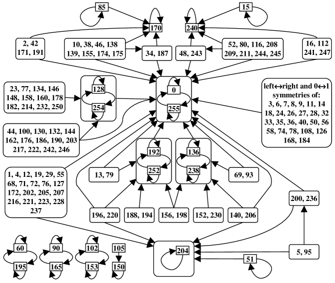
Figure 1: Coarse-graining transitions within the family of 256 elementary CA. Only transitions with a supercell size $N=2,3,4$ are shown. An arrow indicates that the origin rules can be coarse-grained by the target rules and may correspond to several choices of $N$ and $P$.

Several features of Fig. 1 are worthy of a short discussion. First, notice that the map manifests the “left”$\leftrightarrow$“right” and “0”$\leftrightarrow$“1” symmetries of the elementary CA family. For example rules 252, 136 and 238 are the “0”$\leftrightarrow$“1”, “left”$\leftrightarrow$“right” and the “0”$\leftrightarrow$“1” and “left”$\leftrightarrow$“right” symmetries of rule 192 respectively. Second, coarse-graining transitions are obviously transitive, i.e. if $A$ goes to $B$ with $N_{1}$ and $B$ goes to $C$ with $N_{2}$ then $A$ goes to $C$ with $N\leq N_{1}\cdot N_{2}$. For some transitions, the map in Fig. 1 fails to show this property because we did not attain large enough values of $N$.

Another interesting feature of the transition map is that the apparent rule complexity never increases with a coarse-graining transition. Namely, we never find a simple behaving rule which after being coarse-grained becomes a complex rule. The transition map, therefore, introduces a hierarchy of elementary rules and this hierarchy agrees well with the apparent rule complexity. The hierarchy is partial and we cannot relate rules which are not connected by a coarse-graining transition. As opposed to the Wolfram classification, this coarse-graining hierarchy is well defined and is therefore a good candidate for a complexity measureGutowitz (1988, 1990); Binder (1991); Dubacq et al. (2001); Stuner (1990); Culik and Yu (1988); Braga et al. (1995); Jin and Kim (2003); Langton (1990); Wolfram (1984a).

Finally notice that the eight rules 0, 60, 90, 102, 150, 170, 204, 240, whose update function has the additive form

$$f_{\alpha\beta\gamma}\left[x_{n-1},x_{n},x_{n+1}\right] = \alpha\cdot x_{n-1}\oplus\beta\cdot x_{n}\oplus\gamma\cdot x_{n+1}\;,$$ (20)

$$\alpha,\beta,\gamma\in\{0,1\}\;,$$

where $\oplus$ denotes the XOR operation, are all fixed points of the map. This result is not limited to elementary rules. As showed by Barbe et.al Barbe et al. (1995); Barbe (1996, 1997), additive CA in arbitrary dimension whose alphabet sizes are prime numbers coarse-grain themselves. We conjecture that there are situations where reducible fixed points exist for a wide range of systems, analogous to the emergence of amplitude equations in the vicinity of bifurcation points.

When projecting back on the binary alphabet, one maximizes the amount of information lost in the coarse-graining transition. At first glance, this seems to be an unlikely strategy, because it is difficult for the coarse-grained CA to emulate the original one when so much information was lost. In terms of our coarse-graining procedure such a projection maximizes the number of instances $P(x)=P(y)$ of Eq. (4). On second examination, however. this strategy is not that poor. The fact that there are only two states in the coarse-grained alphabet reduces the probability that an instance $P(x)=P(y)$ of Eq. (4) will be violated to 1/2. The extreme case of this argument would be a projection on a coarse-grained alphabet with a single state. Such a trivial projection will never violate Eq. (4) (but will never show any patterns or dynamics either).

A second search strategy for valid projection operators that we used is located on the other extreme of the above tradeoff. Namely, we attempt to lose the smallest possible amount of information. We start by choosing two supercell states $z_{1}$ and $z_{2}$ and unite them using

$$P_{0}\left(x\right)=\left\{\begin{array}[]{l}x\;,\;x\neq z_{2}\\ z_{1}\;,\;x=z_{2}\\ \end{array}\right.\;,$$ (21)

where the subscript in $P_{0}$ denotes that this is an initial trial projection to be refined later. The refinement process of the projection operator proceeds as follows. If $P_{n}$ (starting with $n=0$) satisfies Eq. (4) then we are done. If on the other hand, Eq. (4) is violated by some

$$P_{n}\left(f_{A^{N}}\left[x_{1},x_{2},x_{3}\right]\right) \neq P_{n}\left(f_{A^{N}}\left[y_{1},y_{2},y_{3}\right]\right)\;,$$ (22)

$$P_{n}(x_{i})=P_{n}(y_{i})\;,$$

the inequality is resolved by refining $P_{n}$ to

$$P_{n+1} \left(x\right)=\left\{\begin{array}[]{l}P_{n}\left(x\right)\;,\;x\neq r_{2}\\ P_{n}\left(r_{1}\right)\;,\;x=r_{2}\\ \end{array}\right.\;,$$ (25)

$$r_{1} = f_{A^{N}}\left[x_{1},x_{2},x_{3}\right]\;\;,r_{2}=f_{A^{N}}\left[y_{1},y_{2},y_{3}\right]\;.$$ (26)

This process is repeated until Eq. (4) is satisfied. A non-trivial coarse-graining is found in cases where the resulting projection operator is non-constant (more than a single state in the coarse-grained CA).

By trying all possible $z_{1},z_{2}$ initial pairs, the above projection search method is guaranteed to find a valid projection if such a projection exist on the scale defined by the supercell size $N$. Using this method we were able to coarse-grain many CA. The resulting coarse-grained CA that are generated in this way are often multicolored and do not belong to the elementary CA family. For this reason it is difficult to graphically summarize all the transitions that we found in a map. Instead of trying to give an overall view of those transitions we will concentrate our attention on several interesting cases which we include in the examples section bellow.

IV.2 Examples

IV.2.1 Rule 105

As our first example we choose a transition between two class 2 rules. The elementary rule 105 is defined on the alphabet $\{\square,\blacksquare\}$ with the transition function

$$f_{105}\left[x_{n-1},x_{n},x_{n+1}\right]=\overline{x_{n-1}\oplus x_{n}\oplus x_{n+1}}\;,$$ (27)

where the over-bar denotes the NOT operation, and $\square=0$, $\blacksquare=1$. We use a supercell size $N=2$ and calculate the transition function $f_{105}^{2}$, defined on the alphabet $\{\square\square,\square\blacksquare,\blacksquare\square,\blacksquare\blacksquare\}$. Now we project this alphabet back on the $\{\square,\blacksquare\}$ alphabet with

$$P\left(x\right)=\left\{\begin{array}[]{ll}\square,&x=\square\blacksquare,\blacksquare\square\\ \blacksquare,&x=\square\square,\blacksquare\blacksquare\end{array}\right.\;.$$ (28)

A pair of cells in rule 105 are coarse-grained to a single cell and the value of the coarse cell is black only when the pair share a same value. Using the above projection operator we construct the transition function of the coarse CA. The result is found to be the transition function of the additive rule 150:

$$f_{150}\left[x_{n-1},x_{n},x_{n+1}\right]=x_{n-1}\oplus x_{n}\oplus x_{n+1}\;.$$ (29)

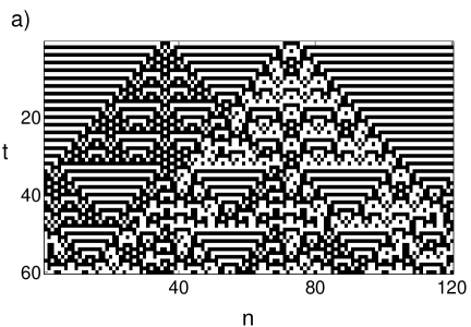
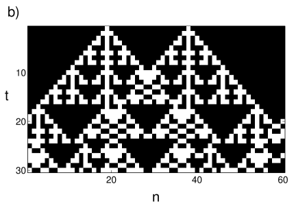
Figure 2: Coarse-graining of rule 105 by rule 150. (a) shows results of running rule 105. The top line is the initial condition and time progress from top to bottom. (b) shows the results of running rule 150 with the coarse grained initial condition from (a).

Figure 2 shows the results of this coarse-graining transition. In Fig. 2 (a) we show the evolution of rule 105 with a specific initial condition while Fig. 2 (b) shows the evolution of rule 150 from the coarse-grained initial condition. The small scale details in rule 105 are lost in the transformation but extended white and black regions are coarse-grained to black regions in rule 150. The time evolution of rule 150 captures the overall shape of these large structures but without the black-white decorations. As shown in Fig. 1, rule 150 is a fixed point of the transition map. Rule 105 can therefore be further coarse-grained to arbitrary scales.

IV.2.2 Rule 146

As a second example of coarse-grained-able elementary CA we choose rule 146. Rule 146 is defined on the $\{\square,\blacksquare\}$ alphabet with the transition function

$$f_{146}\left[x_{n-1},x_{n},x_{n+1}\right]=$$ (32)

$$\left\{\begin{array}[]{l}\blacksquare\;,\;x_{n-1}x_{n}x_{n+1}=\square\square\blacksquare;\blacksquare\square\square;\blacksquare\blacksquare\blacksquare\\ \square\;,\;\mbox{all other combinations}\\ \end{array}\right.\;.$$

It produces a complex, seemingly random behavior which falls into the class 3 group. We choose a supercell size $N=3$ and calculate the transition function $f_{146}^{3}$, defined on the alphabet $\{\square\square\square,\square\square\blacksquare,\dots\blacksquare\blacksquare\blacksquare\}$. Now we project this alphabet back on the $\{\square,\blacksquare\}$ alphabet with

$$P\left(x\right)=\left\{\begin{array}[]{ll}\square,&x\neq\blacksquare\blacksquare\blacksquare\\ \blacksquare,&x=\blacksquare\blacksquare\blacksquare\end{array}\right.\;.$$ (33)

Namely, a triplet of cells in rule 146 are coarse-grained to a single cell and the value of the coarse cell is black only when the triplet is all black. Using the above projection operator we construct the transition function of the coarse CA. The result is found to be the transition function of rule 128 which was given in Eq. (9). Rule 146 can therefore be coarse-grained by rule 128, a class 1 elementary CA. In Figure 3 we show the results of this coarse-graining. Fig. 3 (a) shows the evolution of rule 146 with a specific initial condition while Fig. 3 (b) shows the evolution of rule 128 from the coarse-grained initial condition. Our choice of coarse-graining has eliminated the small scale details of rule 146. Only structures of lateral size of three or more cells are accounted for. The decay of such structures in rule 146 is accurately described by rule 128.

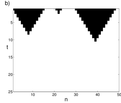
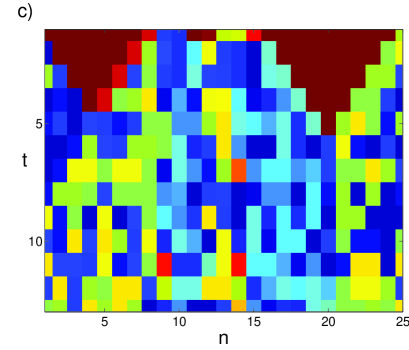
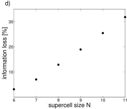
Figure 3: (Color online) Coarse-graining of rule 146 by rule 128 and by a 62 color CA. (a) shows results of running rule 146. The top line is the initial condition and time progress from top to bottom. (b) shows the results of running rule 128 with the coarse grained initial condition from (a). (c) shows results of running the 62 color CA which is a coarse-grained version of rule 146. (d) shows the percentage of supercell states that can be eliminated when coarse graining rule 146 with different supercell sizes $N$.

Note that a class 3 CA was coarse-grained to a class 1 CA in the above example. Our gain was therefore two-fold. In addition to the phase space reduction associated with coarse-graining we have also achieved a reduction in complexity. Our procedure was able to find predictable coarse-grained aspects of the dynamics even though the small scale behavior of rule 146 is complex, potentially irreducible.

Rule 146 can also be coarse-grained by non elementary CA. Using a supercell size of $N=6$ we found that the difference between the combinations $\square\blacksquare\blacksquare\blacksquare\blacksquare\square$ and $\square\blacksquare\square\square\blacksquare\square$ is irrelevant to the long time behavior of rule 146. It is therefore possible to project these two combinations into a single coarse grained state. The same is true for the combinations $\square\blacksquare\blacksquare\square\blacksquare\square$ and $\square\blacksquare\square\blacksquare\blacksquare\square$ which can be projected to another coarse-grained state. The end result of this coarse-graining (Fig. 3 (c)) is a 62 color CA which retains the information of all other 6 cell combinations. The amount of information lost in this transition is relatively small, 2/64 of the supercell states have been eliminated. More impressive alphabet reductions can be found by going to larger scales. For $N$=7,8,9,10 and 11 we found an alphabet reduction of 9/128, 33/256, 97/512, 261/1024 and 652/2048 respectively. Fig. 3 (d) shows the percentage of states that can be eliminated as a function of the supercell size $N$. All of the information lost in those coarse-grainings corresponds to irrelevant DOF.

The two different coarse-graining transitions of rule 146 that we presented above are a good opportunity to show the difference between relevant and irrelevant DOF. As we explained earlier, a transition like 146$\rightarrow$128 where the rules has different complexities must involve the elimination of relevant DOF. Indeed if we modify an initial condition of rule 146 by replacing a $\square\blacksquare\square$ segment with $\square\blacksquare\blacksquare$ we will get a modified evolution. As we show in Figure 4, the difference in the trajectories has a complex behavior and is unbounded in space and time. However, since $\square\blacksquare\square$ and $\square\blacksquare\blacksquare$ are both projected by Eq. (33) to $\square$, the projections of the original and modified trajectories will be identical. In contrast, the coarse graining of rule 146 to the 62 state CA of Fig. 3 (c) involves the elimination of irrelevant DOF only. If we replace a $\square\blacksquare\blacksquare\square\blacksquare\square$ in the initial condition with a $\square\blacksquare\square\blacksquare\blacksquare\square$ we find that the difference between the modified and unmodified trajectories decays after a few time steps.

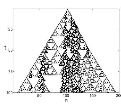
Figure 4: The sensitivity of rule 146 to a relevant DOF change in its initial condition. The figure shows the difference (modulo 2) in the trajectories resulting from replacing a $\square\blacksquare\square$ segment in the initial condition with $\square\blacksquare\blacksquare$.

IV.2.3 Rule 184

The elementary CA rule 184 is a simplified one lane traffic flow model. Its transition function is given by

$$f_{184}\left[x_{n-1},x_{n},x_{n+1}\right]=$$ (36)

$$\left\{\begin{array}[]{l}\square\;,\;x_{n-1}x_{n}x_{n+1}=\square\square\square;\square\square\blacksquare;\square\blacksquare\square;\blacksquare\blacksquare\square\\ \blacksquare\;,\;x_{n-1}x_{n}x_{n+1}=\square\blacksquare\blacksquare;\blacksquare\square\square;\blacksquare\square\blacksquare;\blacksquare\blacksquare\blacksquare\\ \end{array}\right.\;.$$

Identifying a black cell with a car moving to the right and a white cell with an empty road segment we can rewrite the update rule as follows. A car with an empty road segment to its right advances and occupies the empty segment. A car with another car to its right will avoid a collision and stay put. This is a deterministic and simplified version of the more realistic Nagel Schreckenberg model Nagel and Schreckenberg (1992).

Rule 184 can be coarse-grained to a 3 color CA using a supercell size $N=2$ and the local density projection

$$P\left(x\right)=\left\{\begin{array}[]{l}\square\;,\;x=\square\square\\ \color[rgb]{0.4,0.4,0.4}\blacksquare\color[rgb]{0,0,0}\;,\;x=\square\blacksquare;\blacksquare\square\\ \blacksquare\;,\;x=\blacksquare\blacksquare\\ \end{array}\right.\;.$$ (37)

The update function of the resulting CA is given by

$$f\left[y_{n-1},y_{n},y_{n+1}\right]=$$ (42)

$$\left\{\begin{array}[]{l}\square\;,\;y_{n-1}y_{n}y_{n+1}=\square\square\square;\square\square\color[rgb]{0.4,0.4,0.4}\blacksquare\color[rgb]{0,0,0};\square\square\blacksquare;\square\color[rgb]{0.4,0.4,0.4}\blacksquare\color[rgb]{0,0,0}\square;\square\color[rgb]{0.4,0.4,0.4}\blacksquare\color[rgb]{0,0,0}\color[rgb]{0.4,0.4,0.4}\blacksquare\color[rgb]{0,0,0}\\ \blacksquare\;,\;y_{n-1}y_{n}y_{n+1}=\square\blacksquare\blacksquare;\color[rgb]{0.4,0.4,0.4}\blacksquare\color[rgb]{0,0,0}\color[rgb]{0.4,0.4,0.4}\blacksquare\color[rgb]{0,0,0}\blacksquare;\color[rgb]{0.4,0.4,0.4}\blacksquare\color[rgb]{0,0,0}\blacksquare\blacksquare;\blacksquare\color[rgb]{0.4,0.4,0.4}\blacksquare\color[rgb]{0,0,0}\blacksquare;\blacksquare\blacksquare\blacksquare\\ \color[rgb]{0.4,0.4,0.4}\blacksquare\color[rgb]{0,0,0}\;,\;\mbox{all other combinations}\\ \end{array}\right..$$

Figure 5 shows the result of this coarse-graining. Fig. 5 (a) shows a trajectory of rule 184 while Fig. 5 (b) shows the trajectory of the coarse CA. From this figure it is clear that the white zero density regions correspond to empty road and the black high density regions correspond to traffic jams. The density 1/2 grey regions correspond to free flowing traffic with an exception near traffic jams due to a boundary effect.

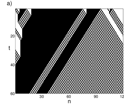
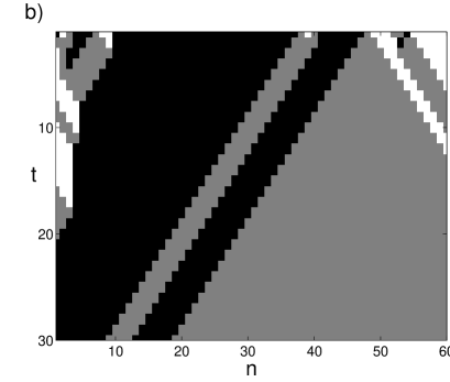
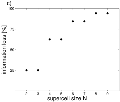
Figure 5: Coarse graining of rule 184 by a 3 state CA. (a) shows a trajectory of rule 184. (b) shows the corresponding trajectory of the coarse-grained CA. (c) shows the percentage of supercell states that can be eliminated when coarse graining rule 184 with different supercell sizes $N$.

By using larger supercell sizes it is possible to find other coarse-grained versions of rule 184. As in the above example, the coarse-grained states group together local configurations of equal car densities. The projection operators however are not functions of the local density alone. They are a partition of such a function and there could be several coarse-grained states which correspond to the same local car density. We found (empirically) that for even supercell sizes $N=2k$ the coarse-grained CA contain $k^{2}/2+3k/2+1$ states and for odd supercell sizes $N=2k+1$ they contain $k^{2}+3k+2$ states. Figure 5 (c) shows the amount of information lost in those transitions as a function of $N$. Most of the lost information corresponds to relevant DOF but some of it is irrelevant.

IV.2.4 Rule 110

Rule 110 is one of the most interesting rules in the elementary CA family. It belongs to class 4 and exhibits a complex behavior where several types of “particles” move and interact above a regular background. The behavior of these “particles” is rich enough to support universal computation Wolfram (2002). In this sense rule 110 is maximally complex because it is capable of emulating all computations done by other computing devices in general and CA in particular. As a consequence it is also undecidable Wolfram (1984b).

We found several ways to coarse-grain rule 110. Using $N=6$, it is possible to project the 64 possible supercell states onto an alphabet of 63 symbols. Figure 6 (a) and (b) shows a trajectory of rule 110 and the corresponding trajectory of the coarse-grained 63 states CA. A more impressive reduction in the alphabet size is obtained by going to larger values of $N$. For $N=7,8,9,10,11,12$ we found an alphabet reduction of $6/128$, $22/256$, $67/512$, $182/1024$, $463/2048$ and $1131/4096$ respectively. Only irrelevant DOF are eliminated in those transitions. Fig. 6 (c) shows the percentage of reduced states as a function of the supercell size $N$. We expect this behavior to persist for larger values of $N$.

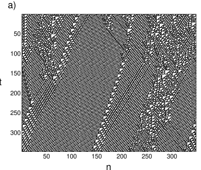
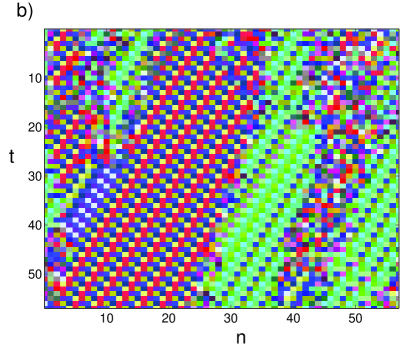
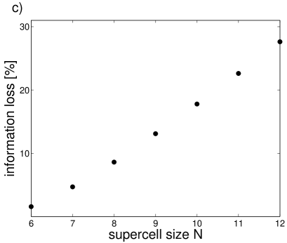
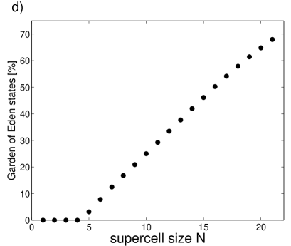
Figure 6: (Color online) Coarse graining of rule 110. (a) shows a trajectory of rule 110. (b) shows a coarse graining of rule 110 by a 63 color CA. (c) shows the percentage of supercell states that can be eliminated when coarse graining rule 110 with different supercell sizes $N$. (d) shows the percentage of “Garden of Eden” states out of the $2^{N}$ possible states of supercell $N$ versions of rule 110.

Another important coarse-graining of rule 110 that we found is the transition to rule 0. Rule 0 has the trivial dynamics where all initial states evolve to the null configuration in a single time step. The transition to rule 0 is possible because many cell sequences cannot appear in the long time trajectories of rule 110. For example the sequence $\square\blacksquare\square\blacksquare\square$ is a so called “Garden of Eden” of rule 110. It cannot be generated by rule 110 and can only appear in the initial state. Coarse-graining by rule 0 is achieved in this case using $N=5$ and projecting $\square\blacksquare\square\blacksquare\square$ to $\blacksquare$ and all other five cell combinations to $\square$. Another example is the sequence $\square\blacksquare\square\blacksquare\blacksquare\square\square\square\blacksquare\blacksquare\square\square\blacksquare$. This sequence is a “Garden of Eden” of the $N=13$ supercell version of rule 110. It can appear only in the first 12 time steps of rule 110 but no later. Coarse-graining by rule 0 is achieved in this case using $N=13$ and projecting $\square\blacksquare\square\blacksquare\blacksquare\square\square\square\blacksquare\blacksquare\square\square\blacksquare$ to $\blacksquare$ and all other 13 cell combinations to $\square$. These examples are important because they show that even though rule 110 is undecidable it has decidable and predictable coarse-grained aspects (however trivial). To our knowledge rule 110 is the only proven undecidable elementary CA and therefore this is the only (proven) example of undecidable to decidable transition that we found within the elementary CA family.

It is interesting to note that the number of “Garden of Eden” states in supercell versions of rule 110 grows very rapidly with the supercell size $N$. As we show in Fig. 6 (d), the fraction of “Garden of Eden” states out of the $2^{N}$ possible sequences, grows almost linearly with $N$. In addition, at every scale $N$ there are new “Garden of Eden” sequences which do not contain any smaller “Gardens of Eden” as subsequences. These results are consistent with our understanding that even though the dynamics looks complex, more and more structure emerges as one goes to larger scales. We will have more to say about this in section V.

The “Garden of Eden” states of supercell versions of rule 110 represent pieces of information that can be used in reducing the computational effort in rule 110. The reduction can be achieved by truncating the supercell update rule to be a function of only non “Garden of Eden” states. The size of the resulting rule table will be much smaller ($\approx 3\%$ with $N=21$) than the size of the supercell rule table. Efficient computations of rule 110 can then be carried out by running rule 110 for the first $N$ time steps. After $N$ time steps the system contains no “Garden of Eden” sequences and we can continue to propagate it by using the truncated supercell rule table without loosing any information. Note that we have not reduced rule 110 to a decidable system. At every scale we achieved a constant reduction in the computational effort. Wolfram has pointed out that many irreducible systems have pockets of reducibility and termed such a reduction as “superficial reducibility” (see page 746 in Ref. Wolfram, 2002). It will be interesting to check how much “superficial reducibility” is contained in rule 110 at larger scales. It will be inappropriate to call it “superficial” if the curve in Fig. 6 (d) approaches 100% in the large $N$ limit.

IV.2.5 Albert and Culik universal CA

It might be argued that the coarse-graining of rule 110 by rule 0 is a trivial example of an undecidable to a decidable coarse-graining transition. The fact that certain configurations cannot be arrived at in the long time behavior is not very surprising and is expected of any irreversible system. In order to search for more interesting examples we studied other one dimensional universal CA that we found in the literature. Lindgren and Nordahl Lindgren and G. (1990) constructed a 7 state nearest neighbor and a 4 state next-nearest neighbor CA that are capable of emulating a universal Turing machine. The entries in the update tables of these CA are only partly determined by the emulated Turing machine and can be completed at will. We found that for certain completion choices these two universal CA can be coarse-grained to a trivial CA which like rule 0 decay to a quiescent configuration in a single time step. Another universal CA that can undergo such a transition is Wolfram’s 19 state, next-nearest neighbor universal CA Wolfram (2002). These results are essentially equivalent to the rule 110 $\rightarrow$ rule 0 transition.

A more interesting example is Albert and Culik’s Albert and K. (1987) universal CA. It is a 14 state nearest-neighbor CA which is capable of emulating all other CA. The transition table of this CA is only partly determined by its construction and can be completed at will. We found that when the empty entries in the transition function are filled by the copy operation

$$f\left[x_{n-1},x_{n},x_{n+1}\right]=x_{n}\;,$$ (43)

the resulting undecidable CA has many coarse-graining transitions to decidable CA. In all these transitions the coarse-grained CA performs the copy operation Eq. (43) for all $\left(x_{n-1},x_{n},x_{n+1}\right)$. Different transitions differ in the projection operator and the alphabet size of the coarse-grained CA. Figure 7 shows a coarse-graining of Albert and Culik’s universal CA to a 4 state copy CA. The coarse-grained CA captures three types of persistent structures that appear in the original system but is ignorant of more complicated details. The supercell size used here is $N=2$.

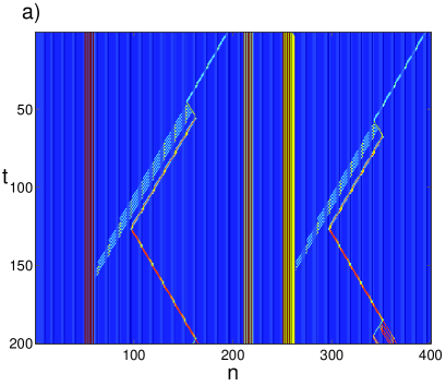
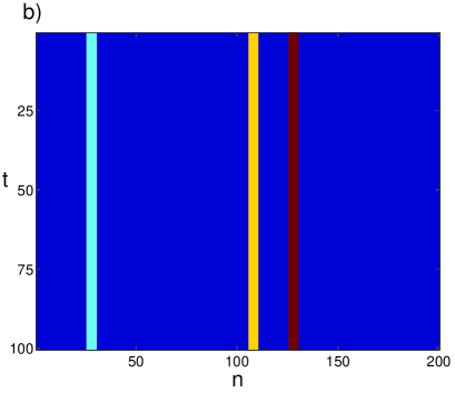
Figure 7: (Color online) Coarse graining of Albert and Culik’s Albert and K. (1987) 14 states universal CA by a 4 state copy CA. (a) shows a trajectory of Albert and Culik’s universal CA while (b) shows the corresponding trajectory of the coarse-grained CA. The supercell size used here is $N=2$

V Coarse-grain-ability of local processes

In the previous section we showed that a large majority of elementary CA can be coarse-grained in space and time. This is rather surprising since finding a valid projection operator is equivalent to solving Eq. (5) which is greatly over constrained. Solutions for this equation should be rare for random choices of the matrix $A^{N}$. In this section we show that solutions of Eq. (5) are frequent because $A^{N}$ is not random but a highly structured object. As the supercell size $N$ is increased, $A^{N}$ becomes less random and the probability of finding a valid projection approaches unity.

To appreciate the high success rate in coarse-graining elementary CA consider the following statistics. By using supercells of size $N=2$ and considering all possible projection operators $P:\{0\dots 3\}\rightarrow\{0,1\}$ we were able to coarse-grain approximately one third of all 256 elementary CA rules. Recall that the coarse-graining procedure that we use involves two stages. In the first stage we generate the supercell version $A^{N}$, a 4 color CA in the $N=2$ case. In the second stage we look for valid projection operators. 4 color CA that are $N=2$ supercell versions of elementary CA are a tiny fraction of all possible ($4^{(4^{3})}\approx 3\times 10^{38}$) 4 color CA. If we pick a random 4 color CA and try to project it; i.e. attempt to solve Eq. (5) with $A^{N}$ replaced by an arbitrary 4 color CA, we find an average of one solvable instance out of every $\approx 1.6\times 10^{7}$ attempts. This large difference in the projection probability indicates that 4 color CA which are supercells versions of elementary rules are not random. The numbers become more convincing when we go to larger values of $N$ and attempt to find projections to random $2^{N}$ color CA.

To put our arguments on a more quantitative level we need to quantify the information content of supercell versions of CA. An accepted measure in algorithmic information theory for the randomness and information content of an individualent object is its Kolmogorov complexity (algorithmic complexity) Li and Vitanyi (1997); Chaitin (1987). The Kolmogorov complexity $K_{U}(x)$ of a string of characters $x$ with respect to a universal computer $U$ is defined as

$$K_{U}\left(x\right)=\frac{L_{U}(x)}{length(x)}\;,$$ (44)

where $length(x)$ is the length of $x$ in bits and $L_{U}(x)$ is the bit length of the minimal computer program that generates $x$ and halts on $U$ (irrespective of the running time). This definition is sensitive to the choice of machine $U$ only up to an additive constant in $L_{U}(x)$ which do not depend on $x$. For long strings this dependency is negligible and the subscript $U$ can be dropped. According to this definition, strings which are very structured require short generating programs and will therefore have small Kolmogorov complexity. For example, a periodic $x$ with period $p$ can be generated by a $\sim p$ long program and $K(x)\sim p/length(x)$. In contrast, if $x$ has no structure it must be generated literally, i.e. the shortest program is “print(x)”. In such cases $L(x)\sim length(x)$, $K(x)\sim 1$ and the information content of $x$ is maximal. By using simple counting arguments Li and Vitanyi (1997) it is easy to show that simple objects are rare and that $K(x)\sim 1$ for most objects $x$. Kolmogorov complexity is a powerful and elegant concept which comes with an annoying limitation. It is uncomputable, i.e. it is impossible to find the length of the minimal program that generates a string $x$. It is only possible to bound it.

It is easy to see that supercell CA are highly structured objects by looking at their Kolmogorov complexity. Consider the CA $A=\left(a\left(t\right),S,f_{A}\right)$ and its $N$’th supercell version $A^{N}=\left(a^{N},S^{N},f_{A^{N}}\right)$ (for simplicity of notation we omit the subscript $A$ from the alphabet size). The transition function $f_{A^{N}}$ is a table that specifies a cell’s new state for all $S^{3N}$ possible local configurations (assuming A is nearest neighbor and one dimensional). $f_{A^{N}}$ can therefore be described by a string of $S^{3N}$ symbols from the alphabet $\{0\dots S^{N}-1\}$. The bit length $length\left(f_{A^{N}}\right)$ of such a description is

$$length\left(f_{A^{N}}\right)=S^{3N}\cdot N\log_{2}{S}\;.$$ (45)

If $A^{N}$ was a typical CA with $S^{N}$ colors we could expect that $L\left(f_{A^{N}}\right)$, the length of the minimal program that generates $f_{A^{N}}$, will not differ significantly from $length\left(f_{A^{N}}\right)$. However, since $A^{N}$ is a super cell version of $A$ we have a much shorter description, i.e. to construct $A^{N}$ from $A$. This construction involves running $A$, $N$ time steps for all possible initial configurations of $3N$ cells. It can be conveniently coded in a program as repeated applications of the transition function $f_{A}$ within several loops. Up to an additive constantLi and Vitanyi (1997), the length of such a program will be equal to the bit length description of $f_{A}$:

$$\tilde{L}\left(f_{A^{N}}\right)=S^{3}\cdot log_{2}{S}\;.$$ (46)

Note that we have used $\tilde{L}$ to indicate that this is an upper bound for the length of the minimal program that generates $f_{A^{N}}$. This upper bound, however, should be tight for an update rule $f_{A}$ with little structure. The Kolmogorov complexity of $f_{A^{N}}$ can consequently be bounded by

$$K\left(f_{A^{N}}\right)\leq\tilde{K}\left(f_{A^{N}}\right)=\frac{\tilde{L}\left(f_{A^{N}}\right)}{length\left(f_{A^{N}}\right)}=N^{-1}\cdot S^{3(1-N)}\;.$$ (47)

This complexity approaches zero at large values of $N$.

Our argument above shows that the large scale behavior of CA (or any local process) must be simple in some sense. We would like to continue this line of reasoning and conjecture that the small Kolmogorov complexity of the large scale behavior is related to our ability to coarse-grain many CA. At present we are unable to prove this conjecture analytically, and must therefore resort to numerical evidence which we present below.

V.1 Garden of Eden states of supercell CA

Ideally, in order to show that such a connection exists one would attempt to coarse-grain CA with different alphabets and on different length scales (supercell sizes), and verify that the success rate correlates with the Kolmogorov complexity of the generated supercell CA. This, however, is computationally very challenging and going beyond CA with a binary alphabet and supercell sizes of more than $N=4$ is not realistic. A more modest experiment is the following. We start with a CA $A$ with an alphabet $S$, and check whether its $N$ supercell version $A^{N}$ contains all possible $S^{N}$ states. Namely, if there exist $x\in\{0\dots S^{N}-1\}$ such that

$$f_{A^{N}}(y_{1},y_{2},y_{3})\neq x\;,\forall y_{1},y_{2},y_{3}\in\{0\dots S^{N}-1\}\;.$$ (48)

Such a missing state of $A^{N}$ is sometimes referred to as a “Garden of Eden” configuration because it can only appear in the initial state of $A^{N}$. Note that by the construction of $A^{N}$, a “Garden of Eden” state of $A^{N}$ can appear only in the first $N-1$ time steps of $A$ and is therefore a generalized “Garden of Eden” of $A$. In cases where a state of $A^{N}$ is missing, $A$ can be trivially coarse-grained to the elementary CA rule 0 by projecting the missing state of $A^{N}$ to “1” and all other combinations to “0”. This type of trivial projection was discussed earlier in connection with the coarse-graining of rule 110. Finding a “Garden of Eden” state of $A^{N}$ is computationally relatively easy because there is no need to calculate the supercell transition function $f_{A^{N}}$. It is enough to back-trace the evolution of $A$ and check if all $N$ cell combinations has a $3N$ cell ancestor combination, $N$ time steps in the past.

Figure 8 (a) shows the statistics obtained from such an experiment. It exhibits the fraction $R_{ge}$ of CA rules with different alphabet sizes $S$, whose $N$’th supercell version is missing at least one state. Each data point in this figure was obtained by testing 10,000 CA rules. The fraction $R_{ge}$ approaches unity at large values of $N$, an expected behavior since most of the CA are irreversible.

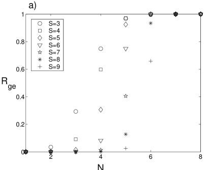
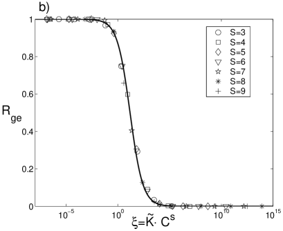
Figure 8: (a) The fraction $R_{ge}$ of CA whose $N$’th supercell version has at least one missing state. Different symbols correspond to different alphabet sizes $S$ of the original CA. (b) Data collapse of the curves $R_{ge}(N,S)$ from a) when plotted against the scaling variable $\xi=\tilde{K}(N,S)\cdot C^{S}$. The solid line shows that the scaling function can be fitted by Eq. (49).

Figure 8 (b) shows the same data as in (a) when plotted against the variable $\xi=\tilde{K}\cdot C^{S}$ where $S$ is the alphabet size, $\tilde{K}$ is the upper bound for the Kolmogorov complexity of the supercell CA from Eq. (47) and $C$ is a constant. The excellent data collapse imply a strong correlation between the probability of finding a missing state and the Kolmogorov complexity of a supercell CA. This figure also shows that the data points can be accurately fitted by

$$R_{ge}\left(N,S\right)=\frac{1}{1+\left(\xi/\xi_{0}\right)^{\alpha}}\;,$$ (49)

with $\xi_{0}$ a constant and $\alpha\approx 0.7$ (solid line in Fig. 8 (b)).

Having the scaling form

$$R_{ge}\left(N,S\right) = F\left(\xi\right)\;,$$ (50)

$$\xi = \tilde{K}\left(N,S\right)\cdot C^{S}=N^{-1}\cdot S^{3(1-N)}\cdot C^{S}\;.$$

we can now study the behavior of $R_{ge}$ with large alphabet sizes. Assuming $F$ and $\xi$ to be continuous we define $\xi_{h}$ as the point where $F\left(\xi_{h}\right)=1/2$. For a fixed value of $S$, the slope of $R_{ge}$ at the transition region can be calculated by

$$\left.\frac{\partial R_{ge}}{\partial N}\right|_{N(\xi_{h})}=F^{\prime}\left(\xi_{h}\right)\cdot\left.\frac{\partial\xi}{\partial N}\right|_{N(\xi_{h})}=$$ (51)

$$-F^{\prime}\left(\xi_{h}\right)\cdot\left(N(\xi_{h})^{-1}+3\log{S}\right)\cdot\xi_{h}\;,$$

where

$$N(\xi_{h}) = \frac{3\log{S}+S\cdot\log{C}-\log{\xi_{h}}-\log{N(\xi_{h})}}{3\cdot\log{S}}$$ (52)

$$\sim \frac{S}{\log{S}}\;.$$

Putting together Eqs. (51) and (52) we find that the slope of $R_{ge}$ at the transition region grows as $\log{S}$ for large values of $S$. An indication of this phenomena can be seen in Fig. 8 (a) which shows sharper transitions at large values of $S$. In the limit of large $S$, $R_{ge}$ becomes a step function with respect to $N$. This fact introduces a critical value $N_{c}(S)$ such that for $N<N_{c}(S)$ the probability of finding a missing state is zero and for $N\geq N_{c}(S)$ the probability is one. The value of this critical $N$ grows with the alphabet size as $N_{c}(S)\sim S/\log{S}$. Note that $N_{c}(S)$ is an emergent length scale, as it is not present in any of the CA rules, but according to the above analysis will emerge (with probability one) in their dynamics. A direct consequence of the emergence of $N_{c}$ is that a measure 1 of all CA can be coarse-grained to the elementary rule “0” on the coarse-grained scale $N_{c}$.

V.2 Projection probability of CA rules with bounded Kolmogorov complexity

Generalized “Garden of Eden” states are a specific form of emergent pattern that can be encountered in the large scale dynamics of CA. Is the Kolmogorov complexity of CA rules related to other types of coarse-grained behavior? To explore this question we attempted to project (solve Eq. (5)) random CA with bounded Kolmogorov complexities.

To generate a random CA $A=(a(t),S,f_{A})$ with a bounded Kolmogorov complexity we view the update rule $f_{A}$ as a string of $S^{3}\log_{2}{S}$ bits, denote the $i$’th bit by $(f_{A})_{i}$ and apply the following procedure: 1) Randomly pick the first $l$ bits of $f_{A}$. 2) Randomly pick a generating function $G:\{0,1\}^{l}\rightarrow\{0,1\}$. 3) Set the values of all the empty bits of $f_{A}$ by applying $G$:

$$(f_{A})_{i}=G\left[(f_{A})_{i-l},(f_{A})_{i-l+1},\cdots,(f_{A})_{i-1}\right]\;,$$ (53)

starting at $i=l+1$ and finishing at $i=S^{3}\log_{s}{S}$. Up to an additive constant, the length of such a procedure is equal to $l+2^{l}$, the number of random bits chosen. The Kolmogorov complexity of the resulting rule table can therefore be bounded by

$$K\left(f_{A}\right)\leq\bar{K}\left(f_{A}\right)=\frac{l+2^{l}}{S^{3}\log_{2}{S}}\;.$$ (54)

For small values of $l$ this is a reasonable upper bound. However for large values of $l$ this upper bound is obviously not tight since the size of $G$ can be much larger than the length of $f_{A}$.

Using the above procedure we studied the probability of projecting CA with different alphabets and different upper bound Kolmogorov complexities $\bar{K}$. For given values of $S$ and $l$ we generated 10,000 (200 for the $S=32$ case) CA and tried to find a valid projection on the $\{0,1\}$ alphabet. Figure 9 (a) shows the fraction $R_{proj}$ of solvable instances as a function of $\xi=\bar{K}\cdot C^{S}$. The constant $C$ used for this data collapse is $1.02$, very close to $1$. As valid projection solutions we considered all possible projections $P:S^{3}\rightarrow\{0,1\}$. In doing so we may be redoing the missing states experiment because many low Kolmogorov complexity rules has missing states and can thus be trivially projected. In order to exclude this option we repeated the same experiment while restricting the family of allowed projections to be equal partitions of $\{0\cdots S^{3}-1\}$, i.e.

$$P:S^{3}\rightarrow\{0,1\}\;;\;\;|\{x:P(x)=0\}|=|\{x:P(x)=1\}|\;.$$ (55)

The results are shown if Fig. 9 (b).

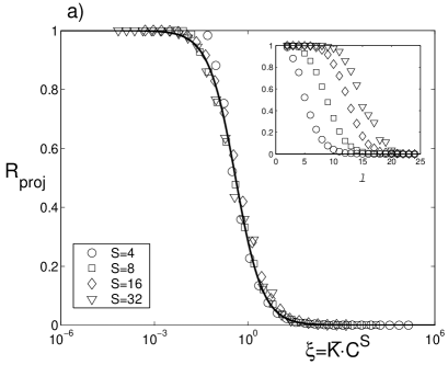
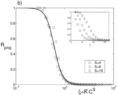
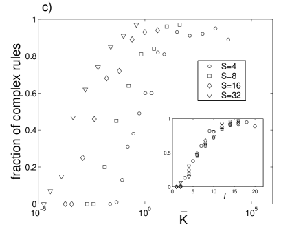
Figure 9: (a) and (b) show the fraction $R_{proj}$ of Kolmogorov complexity bounded CA that has a valid projection on the binary alphabet. CA were generated using a random generating function with $l$ variables according to the procedure described above. $\bar{K}$ (Eq. (54)) is the resulting upper bound Kolmogorov complexity. Different symbols correspond to different alphabet sizes. Insets show the data as a function of the parameter $l$. (a) shows results in the case where all projections $P:S^{3}\rightarrow\{0,1\}$ are allowed. (b) shows results in the case where only equal partition projections (Eq. (55)) are allowed. Solid lines in (a) and (b) shows a fit by Eq. (56). (c) shows the fraction of complex behaving rules which are produced by our procedure as a function of $l$.

It seems that in both cases there is a good correlation between the Kolmogorov complexity (or its upper bound) of a CA rule and the probability of finding a valid projection. In particular, the fraction of solvable instances goes to one at the low $\bar{K}$ limit. As shown by the solid lines in Fig. 9, this fraction can again be fitted by

$$R_{proj}=\frac{1}{1+\left(\xi/\xi_{0}\right)^{\alpha}}\;,$$ (56)

where $\xi_{0}$ is a constant and in this case $\alpha\approx 1$.

How many of the CA rules that we generate and project show a complex behavior? Does the fraction of projectable rules simply reflect the fraction of simple behaving rules? To answer this question we studied the rules generated by our procedure. For each value of $S$ and $l$ we generated 100 rules and counted the number of rules exhibiting complex behavior. A rule was labelled “complex” if it showed class 3 or 4 behavior and exhibited a complex sensitivity to perturbations in the initial conditions. Fig. 9 (c) shows the statistics we obtained with different alphabet sizes as a function of $\bar{K}$ while the inset shows it as a function of $l$. We first note that our statistics support Dubacq et al. Dubacq et al. (2001), who proposed that rule tables with low Kolmogorov complexities lead to simple behavior and rule tables with large Kolmogorov complexity lead to complex behavior. Moreover, our results show that the fraction of complex rules does not depend on the alphabet size and is only a function of $l$. Rules with larger alphabets show complex behavior at a lower value of $\bar{K}$. As a consequence, a large fraction of projectable rules are complex and this fraction grows with the alphabet size $S$.

As we explained earlier, the Kolmogorov complexity of supercell versions of CA approaches zero as the supercell size $N$ is increased. Our experiments therefore indicate that a measure one of all CA are coarse-grained-able if we use a coarse enough scale. Moreover, the data collapse that we obtain and the sharp transition of the scaling function suggest that it may be possible to know in advance at what length scales to look for valid projections. This can be very useful when attempting to coarse-grain CA or other dynamical systems because it can narrow down the search domain. As in the case of “Garden of Eden” states that we studied earlier, we interpret the transition point as an emergent scale which above it we are likely to find self organized patterns. Note however that this scale is a little shifted in Fig. 9 (b) when compared with Fig. 9 (a). The emergence scale is thus sensitive to the types of large scale patterns we are looking for.

VI Summary and discussion

In this work we studied emergent phenomena in complex systems and the associated predictability problems by attempting to coarse-grain CA. We found that many elementary CA can be coarse-grained in space and time and that in some cases complex, undecidable CA can be coarse-grained to decidable and predictable CA. We conclude from this fact that undecidability and computational irreducibility are not good measures for physical complexity. Physical complexity, as opposed to computational complexity should address the interesting, physically relevant, coarse-grained degrees of freedom. These coarse-grained degrees of freedom maybe simple and predictable even when the microscopic behavior is very complex.

The above definition of physical complexity brings about the question of the objectivity of macroscopic descriptions Schulman and Gaveau (2001); Shalizi and Moore (2004). Is our choice of a coarse-grained description (and its consequent complexity) subjective or is it dictated by the system? Our results are in accordance with Shalizi and Moore Shalizi and Moore (2004): it is both. In many cases we discovered that a particular CA can undergo different coarse-graining transitions using different projection operators. In these cases the system dictates a set of valid projection operators and we are restricted to choose our coarse-grained description from this set. We do however have some freedom to manifest our subjective interest.

The coarse-graining transitions that we found induce a hierarchy on the family of elementary CA (see Fig. 1). Moreover, it seems that rule complexity never increases with coarse-graining transitions. The coarse-graining hierarchy therefore provides a partial complexity order of CA where complex rules are found at the top of the hierarchy and simple rules are at the bottom. The order is partial because we cannot relate rules which are not connected by coarse-graining transitions. This coarse-graining hierarchy can be used as a new classification scheme of CA. Unlike Wolfram’s, classification this scheme is not a topological one since the basis of our suggested classification is not the CA trajectories. Nor is this scheme parametric, such as Langton’s $\lambda$ parameter scheme. Our scheme reflects similarities in the algebraic properties of CA rules. It simply says that if some coarse-grained aspects of rule $A$ can be captured by the detailed dynamics of rule $B$ then rule $A$ is at least as complex as rule $B$. Rule $A$ maybe more complex because in some cases it can do more than its projection. Note that our hierarchy may subdivide Wolfram’s classes. For example rule 128 is higher on the hierarchy than rule 0. These two rules belong to class 1 but rule 128 can be coarse-grained to rule 0 and it is clear that an opposite transition cannot exist. It will be interesting to find out if class 3 and 4 can also be subdivided.

In the last part of this work we tried to understand why is it possible to find so many coarse-graining transitions between CA. At first blush, it seems that coarse-graining transitions should be rare because finding valid projection operators is an over constrained problem. This was our initial intuition when we first attempted to coarse-grain CA. To our surprise we found that many CA can undergo coarse-graining transitions.

A more careful investigation of the above question suggests that finding valid projection operators is possible because of the structure of the rules which govern the large scale dynamics. These large scale rules are update functions for supercells, whose tables can be computed directly from the single cell update function. They thus contain the same amount of information as the single cell rule. Their size however grows with the supercell size and therefore they have vanishing Kolmogorov Complexities.

In other words, the large scale update functions are highly structured objects. They contain many regularities which can be used for finding valid projection operators. We did not give a formal proof for this statement but provided a strong experimental evidence. In our experiments we discovered that the probability to find a valid projection is a universal function of the Kolmogorov Complexity of the supercell update rule. This universal probability function varies from zero at large Kolmogorov Complexity (small supercells) to one at small Kolmogorov Complexity (large supercells). It is therefore very likely that we find many coarse-graining transitions when we go to large enough scales.

Our interpretation of the above results is that of emergence. When we go to large enough scales we are likely to find dynamically identifiable large scale patterns. These patterns are emergent (or self organized) because they do not explicitly exist in the original single cell rules. The large scale patterns are forced upon the system by the lack of information. Namely, the system (the update rule, not the cell lattice) does not contain enough information to be complex at large scales.

Finding a projection operator is one specific type of an over constrained problem. Motivated by our results we looked into other types of over constrained problems. The satisfyabilityKirkpatrick and Selman (1994); Monasson et al. (1999) problem (k-sat) is a generalized (NP complete) form of constraint satisfaction system. We generated random 3-sat instances with different number of variables deep in the un-sat region of parameter space. The generated instances however were not completely random and were generated by generating functions. The generating functions controlled the instance’s Kolmogorov complexity, in the same way that we used in section V.2. We foundunp that the probability for these instances to be satisfiable obeys the same universal probability function of Eq. (56). It will be interesting to understand the origin of this universality and its implications.

In this work, we have restricted ourselves to deal with CA because it is relatively easy to look for valid projection operators for them. A greater (and more practical) challenge will now be to try and coarse-grain more sophisticated dynamical systems such as probabilistic CA, coupled maps and partial differential equations. These types of systems are among the main work horses of scientific modelling, and being able to coarse-grain them will be very useful, and is a topic of current research, e.g. in material scienceGoldenfeld et al. (2005). It will be interesting to see if one can derive an emergence length scale for those systems like the one we found for “Garden of Eden” sequences in CA (section V.1). Such an emergence length scale can assist in finding valid projection operators by narrowing the search to a particular scale.