Chaotic advection and targeted mixing

Abstract

The advection of passive tracers in an oscillating vortex chain is investigated. It is shown that by adding a suitable perturbation to the ideal flow, the induced chaotic advection exhibits two remarkable properties compared with a generic perturbation : Particles remain trapped within a specific domain bounded by two oscillating barriers (suppression of chaotic transport along the channel), and the stochastic sea seems to cover the whole domain (enhancement of mixing within the rolls).

In order to enhance mixing in flows one often relies on chaotic advection Ar . This phenomenon translates the fact that despite the laminar character of a given flow, trajectories of fluid particles or advected passive tracers are chaotic. As a consequence, mixing is considerably enhanced in regions where chaos is at play, as it does not need to rely on molecular diffusion. Such phenomena are observed in a wide range of physical systems Ot and have fundamental applications, for instance, in geophysical flows BeMeSw ; BrSm or chemical engineering. When considering two dimensional incompressible flows, chaotic advection occurs when the flow is unsteady, see for instance Refs. SoGo ; SoMiSpMo ; WiCaTA ; CaWi . One peculiarity of these flows is that the dynamics of passive particles can be tackled from the Hamiltonian dynamics point of view. The canonical variables are directly the space variables, hence the phase space is formally the two dimensional physical space. This feature allows a direct visualization of the phase space in experiments, and in a certain sense makes this framework an ideal one in order to confront theoretical results on Hamiltonian dynamics with experiments.

In this Letter, we address the problem of targeted mixing. Namely it is often desirable to reduce chaotic transport (see Ref. CCDLMV ) while one also often wants more chaos in order to enhance mixing (see, for instance, Refs. Ba ; Mez for microfluidic and microchannel devices). In order to achieve such properties, we consider the dynamics of passive tracers in an array of alternating vortices. This flow has been realized experimentally using Rayleigh-Bénard convection or in a more controlled way by using electromagnetic forces SoGo ; SoMiSpMo ; WiCaTA . The primary interest in this flow resides in the fact that being generated by quite a few hydrodynamic instabilities, it may be considered as one of the founding bricks of turbulence. As such, understanding its influence on the advection of passive or active quantities is considered a necessary first step in order to uncover the different mechanisms governing for instance front propagation in turbulent flows AbCeVeVu ; PoHa .

We consider the following integrable stream function which models the experiment with slip boundary conditions :

$$\Psi_{0}(x,y)=\alpha\sin x\sin y,$$ (1)

where the $x$-direction is the horizontal one along the channel and the $y$-direction is the bounded vertical one. The constant $\alpha$ is the maximal value of vertical velocity. Passive particles follow the streamlines of $\Psi_{0}$ depicted on Fig. 1$(a)$. The dynamics given by Eq. (1) is integrable. Therefore no mixing occurs. The fluid is limited by two invariant surfaces $y=\pi$ and $y=0$ corresponding to the top and bottom roll boundaries. The flow has hyperbolic fixed points on these two invariant surfaces which are localized at $x=m\pi$ for $m\in\mathbb{Z}$. These points are joined by vertical heteroclinic connections for which the stable and unstable manifolds coincide. The phase space, which is here the real space, is then characterized by a chain of rolls with separatrices localized at $x=m\pi$ for $m\in\mathbb{Z}$.

In the experiments SoGo ; SoMiSpMo ; WiCaTA , a typical perturbation $f(x,y,t)$ is introduced as a time dependent forcing in order to trigger chaotic advection and then to study the resulting transport and mixing properties. More precisely the perturbation modifies the stream function as :

$$\Psi_{c}(x,y,t)=\Psi_{0}(x+f(x,y,t),y).$$ (2)

For instance, the following stream function has been proposed to model an experimental situation SoGo  :

$$\Psi_{1}(x,y,t)=\alpha\sin(x+\epsilon\sin\omega_{0}t)\sin y,$$ (3)

i.e. the perturbation is $f=\epsilon\sin\omega_{0}t$ and describes the lateral oscillations of the roll patterns where $\epsilon$ and $\omega_{0}$ are respectively the amplitude and the angular frequency of the lateral oscillations. Without loss of generality, we assume that $\omega_{0}=1$. The resulting streamlines which are again closed curves correspond to lateral oscillations in the $x$-direction of the streamlines depicted in Fig. 1$(a)$ with a periodic displacement of $-\epsilon\sin t$. However chaotic advection is triggered.

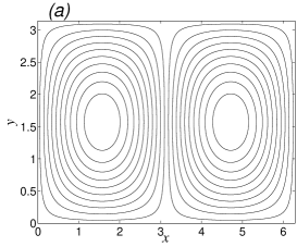
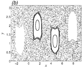
Figure 1: Poincaré sections $(a)$ for the stream function (1) which are also the streamlines and $(b)$ for the stream function (3). The parameters are $\alpha=0.6$ and $\epsilon=0.63$.

In order to infer transport and mixing properties we use Poincaré sections of some trajectories of tracers. A typical Poincaré section associated with the stream function $\Psi_{1}$ given by Eq. (3) is represented in Fig. 1$(b)$ for $\epsilon=0.63$ and $\alpha=0.6$. It shows that the transport along the channel is greatly enhanced SoGo compared with no transport in Fig. 1$(a)$. The advected tracers have now a non integrable Hamiltonian dynamics. The reason being that, under the perturbation, the vertical heteroclinic connections between the vortices break down and the stable and unstable manifolds intersect transversely thus generating chaotic advection of passive tracers along the channel Wi . Therefore the mixing properties of the flow are enhanced. However, most of the time islands of stability remain, among which the ones located around the centers of the vortices. They are characterized by regular (quasiperiodic) trajectories and a chaotic region around and between the rolls. Mixing within the center of the rolls can only rely on molecular diffusion while tracers in the chaotic sea are advected unboundedly along the channel and chaotic mixing occurs. The main observation is that the regular patterns persist and chaos or mixing are not well developed.

In order to obtain what we called targeted mixing, we propose to adjust the time-dependent forcing $f$ which we assume to depend on $y$ and $t$ such that the stream function $\Psi_{c}$ given by Eq. (2) has the following properties : First its attendant chaotic transport along the channel ($x$-direction) is confined by impenetrable barriers. Second, when restricted to each of these independent cells, we want to obtain good mixing properties.

A first possibility to create barriers given by invariant tori of the dynamics would be to use the method proposed in Refs. ViChCiLi ; CCDLMV for controlling Hamiltonian systems. This method uses an affine control (modifying the Hamiltonian or the stream function additively). However applying this method to the system under consideration would create some barriers but would also regularize the inside of the cell, thus drastically reducing the mixing.

In order to proceed in finding a more suitable perturbation $f(y,t)$, we start from a more generic situation for which the stream function given by Eq. (1) is a particular case. We consider a generic integrable stream function $\Psi_{0}(x,y)$ which is $L$-periodic in $x$, and such that $\partial_{x}\Psi_{0}(x,0)=\partial_{x}\Psi_{0}(x,H)=0$ for all $x\in{\mathbb{R}}$ where $H$ is the height of the channel. The perturbed stream function is written as in Eq. (2) where $f(y,t)$ is such that $(i)$ there are barriers at $x=x_{k}(y,t)$ (for $k\in{\mathbb{Z}}$) which prevent the chaotic advection along the $x$-direction and $(ii)$ there is a high mixing inside a region bounded by two consecutive barriers, e.g., $x_{1}$ and $x_{2}$. We notice that the perturbed stream function is obtained by adding the perturbation to the canonical variables of the stream function and not to the stream function itself as in Refs. ViChCiLi ; CCDLMV . The equations of the barriers are written as $x=x_{k}(y,t)=kL+\varphi(y,t)$ for $k\in{\mathbb{Z}}$ where $\varphi$ is a function to be determined. Using Hamilton’s equations

$$\dot{x} = -\frac{\partial\Psi_{c}}{\partial y}=-\frac{\partial\Psi_{0}}{\partial y}(x+f,y)-\frac{\partial f}{\partial y}\frac{\partial\Psi_{0}}{\partial x}(x+f,y)\>,$$

$$\dot{y} = \frac{\partial\Psi_{0}}{\partial x}(x+f,y)\>,$$

and by imposing that $x_{k}$ locates a barrier we get for the particles on the barrier

$$\dot{x}=\frac{\partial\varphi}{\partial t}+\dot{y}\frac{\partial\varphi}{\partial y}\>.$$

Thus a possible solution is obtained when $f+\varphi$ is only a function of time, denoted $\Phi(t)$, and the condition on $\varphi$ is

$$\frac{\partial\varphi}{\partial t}=-\frac{\partial\Psi_{0}}{\partial y}(\Phi(t),y).$$

The above equation is solved as

$$\varphi(y,t)=-\Gamma\partial_{y}\Psi_{0}(\Phi(t),y),$$

where the linear operator $\Gamma$ is a pseudo-inverse of $\partial_{t}$, i.e. acting on $v(y,t)=\sum_{k}v_{k}{\mathrm{e}}^{ikt}$ as

$$\Gamma v=\sum_{k\not=0}\frac{v_{k}}{ik}{\mathrm{e}}^{ikt}.$$

The perturbation $f$ is then

$$f(y,t)=\Phi(t)+\Gamma\partial_{y}\Psi_{0}(\Phi(t),y),$$ (4)

where $\Phi$ is any function of time.

We now apply these results to the array of vortices given by the stream function (1). In order to remain as close as possible to the experimental setup, we consider $\Phi(t)=\epsilon\sin t$.

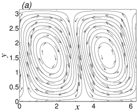
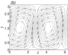
Figure 2: Streamlines of the stream function (5) at $(a)$ $t=0$ and $(b)$ $t=3\pi/4$. The parameters are $\alpha=0.6$ and $\epsilon=0.63$.

The modified stream function given by Eq. (4) is then

$$\Psi_{c}(x,y,t)=\alpha\sin[x+\epsilon\sin t+\alpha\cos yC_{\epsilon}(t)]\sin y,$$ (5)

where

$$C_{\epsilon}(t)=\sum_{n\geq 0}\frac{-2}{2n+1}\mathcal{J}_{2n+1}(\epsilon)\cos(2n+1)t,$$ (6)

and $\mathcal{J}_{l}$ (for $l\in\mathbb{N}$) are Bessel functions of the first kind. We notice that $y=0$ and $y=\pi$ are still boundaries for the streamfunction  (5) which comes from the fact that the modification is only on the $x$-term of the original stream function. The streamlines are then slightly modified (non-uniformly in $y$) as it can be seen on Fig. 2$(a)$ and $(b)$ which depict the streamlines of the stream function (5) for $\epsilon=0.63$ and $\alpha=0.6$ at two different times $t=0$ and $t=3\pi/4$ respectively. Moreover, the displacement of these rolls remains parallel to the $x$-axis as it is for the stream function $\Psi_{1}$ given by Eq. (3). The fact that the streamlines of the stream function (3) and the ones of Eq. (5) look similar comes from the fact that the stream function $\Psi_{c}$ is a small modification of $\Psi_{1}$ (for $\alpha$ small) since we have $\left|\Psi_{c}(x,y,t)-\Psi_{1}(x,y,t)\right|\leq{\alpha^{2}}\epsilon/{2}$.

Nevertheless, the dynamics of tracers is completely different in both cases and targeted mixing is achieved. For the same values of $\epsilon$ and $\alpha$ as in Fig. 1$(b)$,

Figure 3: Poincaré section for the stream function (5). The parameters are $\alpha=0.6$ and $\epsilon=0.63$.

a Poincaré section of the dynamics of passive tracers in a flow described by the stream function $\Psi_{c}$ given by Eq. (5) is represented in Fig. 3. We notice that there are invariant surfaces which have been created around $x=0$ (mod $2\pi$) (bold curves) and that mixing within these barriers is considerably enhanced. The equations of these transport barriers along the $x$-direction are :

$$x=x_{k}(y,t)=2k\pi-\alpha\cos yC_{\epsilon}(t).$$ (7)

To be more specific, the barriers (7) are degenerate invariant tori since each of them is a heteroclinic connexion between two hyperbolic periodic orbits (with period $2\pi$), e.g., one locate at $y=0$ and $x(t)=-\alpha C_{\epsilon}(t)$ and the other one at $y=\pi$ and $x(t)=\alpha C_{\epsilon}(t)$, moving in opposite directions along the channel. Regarding the enhancement of mixing inside the cell bounded by the two barriers observed in Fig. 3, we notice that most of the regular trajectories observed for the stream function $\Psi_{1}$ are broken by the perturbation (in comparison with Fig. 1$(b)$). It means that, the perturbation given by Eq. (4) creates two invariant surfaces around $x=0$ and $x=2\pi$, and destabilizes the inside of the cell and in particular the remainders of the regular motion near $x=\pi/2$ and $x=3\pi/2$.

In order to get some clues on the origin of mixing enhancement, we consider the region in the middle of the cell of length $L$ in the $x$-direction and compute the Melnikov function which measures the distance between the stable and unstable manifolds. First, we perform the (time-dependent) canonical transformation $(x,y)\mapsto(x^{\prime},y^{\prime})$ generated by $F_{2}(y,x^{\prime},t)=yx^{\prime}-\Gamma\Psi_{0}(\Phi(t),y)$. In the case of $\Psi_{0}$ given by Eq. (1), the stream function becomes

$$\tilde{\Psi}_{c}(x^{\prime},y^{\prime},t)=\alpha[\sin(x^{\prime}+\Phi(t))-\sin(\Phi(t))]\sin y^{\prime}.$$

The Melnikov function is defined as CaWi

$$M(t_{0})=\int_{-\infty}^{+\infty}\{\Psi_{0},\tilde{\Psi}_{c}\}(x_{0}(t-t_{0}),y_{0}(t-t_{0}))\,dt,$$

where $(x_{0}(t),y_{0}(t))$ is a solution of the unperturbed system $\Psi_{0}$. The Poisson bracket between $\Psi_{0}$ and $\tilde{\Psi}_{c}$ is given by

$$\{\Psi_{0},\tilde{\Psi}_{c}\}=\alpha^{2}(1-\cos x)\sin(\Phi(t))\sin y\cos y.$$

It is straightforward to see that the Melnikov function vanishes when $x=0\mbox{ mod }2\pi$, i.e. on the boundaries of the cell, and is maximum (in absolute value) when $x=\pi\mbox{ mod }2\pi$, i.e. in the middle of the cell. Therefore it is expected that the mixing is enhanced since then, there is a maximum flux inside the cell Ba .

In order to test the robustness of the method and to try an experimentally more tractable perturbation, we truncate the series given by Eq. (6). The simplest possible perturbation is obtained by considering only the first term of the series $C_{\epsilon}(t)$ in Eq. (6) which leads to the following stream function

$$\Psi_{s}(x,y,t)=\alpha\sin\left(x+\epsilon\sin t-2\alpha\mathcal{J}_{1}(\epsilon)\cos y\cos t\right)\sin y,$$ (8)

which has a much simpler time-dependence. We performed a Poincaré section for this simplified stream function $\Psi_{s}$ given by Eq. (8) for $\alpha=0.6$ and $\epsilon=0.63$. This Poincaré section looks identical to the one depicted on 3 showing that the simplified perturbation remains efficient.

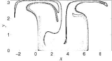
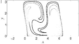
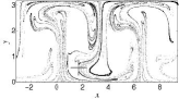
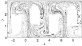
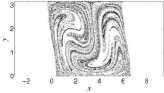
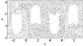
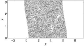
Figure 4: Numerical simulation of the dynamics of a dye at $t=30$, $t=50$, $t=70$ and $t=140$ (from top to bottom) : left column for the stream function (3) and right column for the stream function (5). The parameters are $\alpha=0.6$ and $\epsilon=0.63$.

In Fig. 4, we depict a numerical simulation of the dynamics of a dye in the fluid. The left column shows the evolution of the tracers for the stream function $\Psi_{1}$ given by Eq. (3). The right column shows the mixing of a dye within a cell which is limited by two barriers created by the stream function $\Psi_{c}$ given by Eq. (5). We see that the mixing occurs through a combination of stretching and folding of the dye. The corresponding figure for $\Psi_{s}$ given by Eq. (8) shows some advected particles outside the cell but the same picture inside.

In conclusion, we considered a situation of time-dependent oscillating vortex chain. We have shown by adding a suitable perturbation (forcing) it is possible to suppress the chaotic advection along the channel by creating dynamical barriers among the vortex chain, and at the same time, to enhance the mixing of passive tracers inside each of these isolated cells. The effect is obtained in spite of the oscillations of the rolls and is not too much affected by the use of a simplified version of the exact stream function.

- (1) H. Aref, J. Fluid Mech. 143, 1 (1984).
- (2) J.M. Ottino, The Kinematics of Mixing: Stretching, Chaos and Transport (Cambridge University Press, Cambridge, 1989).
- (3) R.P. Behringer, S. Meyers, H. Swinney, Phys. Fluids A 3, 1243 (1991).
- (4) M.G. Brown, K.B. Smith, Phys. Fluids A 3, 1186 (1991).
- (5) T.H. Solomon, J.P. Gollub, Phys. Rev. A 38, 6280 (1988).
- (6) T.H. Solomon, N.S. Miller, C.J.L. Spohn, J.P. Moeur, AIP Conf. Proc. 676, 195 (2003).
- (7) H. Willaime, O. Cardoso, P. Tabeling, Phys. Rev. E 48, 288 (1993).
- (8) R. Camassa, S. Wiggins, Phys. Rev. A 43, 774 (1991).
- (9) C. Chandre, G. Ciraolo, F. Doveil, R. Lima, A. Macor, M. Vittot, Phys. Rev. Lett. 94, 074101 (2005).
- (10) S. Balasuriya, Physica D 202, 155 (2005).
- (11) A.D. Stroock, S.K.W. Dertinger, A. Ajdari, I. Mezic, H.A. Stone, G.M. Whitesides, Science 295, 647 (2002).
- (12) M. Abel, A. Celani, D. Vergni, A. Vulpiani, Phys. Rev. E 64, 046307 (2001).
- (13) A. Pocheau, F. Harambat, Experimental study of chemical front propagation in a cellular flow preprint (2005); A. Pocheau, F. Harambat, in Proceedings of the 21st International Congress of Theoretical and Applied Mechanics (2004).
- (14) S. Wiggins, Chaotic Transport in Dynamical Systems (Springer-Verlag, Berlin, 1992).
- (15) M. Vittot, C. Chandre, G. Ciraolo, R. Lima, Nonlinearity 18, 423 (2003).