Chaotic and Pseudochaotic Attractors of Perturbed Fractional Oscillator

Abstract

We consider a nonlinear oscillator with fractional derivative of the order $\alpha$. Perturbed by a periodic force, the system exhibits chaotic motion called fractional chaotic attractor (FCA). The FCA is compared to the “regular” chaotic attractor. The properties of the FCA are discussed and the “pseudochaotic” case is demonstrated.

I Introduction

It became evident now that the random dynamics can appear as an intrinsic property of real systems and that different kind of randomness represents a level of complexity of motion. While the Hamiltonian chaos is relevant to the Hamiltonian systems, chaotic properties of the dissipative dynamics are very different revealing the chaotic attractors, strange non-chaotic attractors, quasi-attractors, etc. Ott ; Zaslavsky1978 ; Alligood . In this paper we would like to describe one more way of the occurrence of chaotic or pseudo-chaotic attractors in dissipative systems. Namely, the forced system is a fractional nonlinear oscillator (FNO), i.e. a nonlinear oscillator with a fractional derivative of the order $0<\alpha<2$ with respect to time instead of the second order derivative.

Although the fractional calculus has more than few-hundred-year story, its application to the contemporary physics is very recent and, mainly, it is related to the complexity of the media in classical and quantum treatment. Let us mention only a few of them: fractional kinetics 37 ; rz1 ; Piryatinska , wave propagation in a media with fractal properties rz2 ; rz8 ; rz9 , nonlinear optics Weitzner , quantum mechanics rz3 , quantum field theory rz4 , and many others.The formal issues related to the contemporary fractional calculus are well reflected in the monographs Gelfand ; rz5 ; rz6 ; PodlubnyBook ; 47 . There are different possibilities for interpretation of fractional derivatives. Let us mention the probabilistic interpretation rz6 ; Machado ; rz7 ; Stanislavsky2004 and the relation to a dissipation of the considered system 41 ; Gorenflo ; 34 ; StanislavskyPRE04 . The latter one will be related to our paper.

The paper contains some necessary definitions in Sec. II and in two appendices. In Sec. III we demonstrate how the fractional derivative can be related to a dissipation in the system. The Sec. IV is devoted to the main object of the paper: fractional chaotic attractor (FCA) and some of its features. We speculate on the existence of fractional “pseudochaotic” attractor, i.e. dissipative random dynamics with zero Lyapunov exponent.

II Definitions

In this section we put some necessary definitions. The left ${}_{a}D^{\alpha}_{t}$ and right ${}_{t}D^{\alpha}_{b}$ Riemann-Liouville fractional derivatives of order $\alpha$ are defined as

$${}_{a}D^{\alpha}_{t}f(t)={\frac{1}{\Gamma(n-\alpha)}}{\frac{d^{n}}{dt^{n}}}\int^{t}_{a}(t-\tau)^{n-\alpha-1}f(\tau)d\tau\ ,\$$

$${}_{t}D^{\alpha}_{b}f(t)={\frac{(-1)^{n}}{\Gamma(n-\alpha)}}{\frac{d^{n}}{dt^{n}}}\int^{b}_{t}(\tau-t)^{n-\alpha-1}f(\tau)d\tau\ ,$$ (1)

$$(n-1\leq\alpha\leq n)\ .\$$

To construct a solution for a process described by an equation with fractional derivatives, one needs the initial conditions that can be written as

$$\lim_{t\rightarrow a}{{}_{a}D^{\alpha-k}_{t}}f(t)=a_{k}\ ,\ \ \ \ \ (k=1,2,...,n)$$ (2)

or

$$\lim_{t\rightarrow b}{{}_{t}D^{\alpha-k}_{b}}f(t)=b_{k}\ ,\ \ \ \ \ (k=1,2,...,n)\ .\$$ (3)

These conditions may have no physical meaning (for a detailed discussion see PodlubnyBook ; rz10 ). The important feature of the derivatives (1) is that they have no symmetry with respect to the time reflection $t\rightarrow-t$.

In the following we use the so-called Caputo derivative Rabotnov ; Caputo defined as

$${}_{a}^{C}D^{\alpha}_{t}f(t)={\frac{1}{\Gamma(\alpha-n)}}\int^{t}_{a}(t-\tau)^{n-\alpha-1}f^{(n)}(\tau)d\tau\ ,\$$

$${}_{t}^{C}D^{\alpha}_{b}f(t)={\frac{(-1)^{n}}{\Gamma(\alpha-n)}}\int^{b}_{t}(\tau-t)^{n-\alpha-1}f^{(n)}(\tau)d\tau\ ,$$ (4)

$$(n-1\leq\alpha\leq n)$$

with the regular type of initial conditions

$$f^{(k)}(a)=a_{k}\ \ {\rm or}\ \ f^{(k)}(b)=b_{k}\ ;\ \ \ \ \ k=0,1,...,(n-1)\ .\$$ (5)

For the left Caputo derivative we use a notation

$${}_{0}^{C}D^{\alpha}_{t}\equiv D^{\alpha}\ .\$$ (6)

Left fractional oscillator will be described by the equation:

$${}_{0}D^{\alpha}_{t}x_{1}(t)-\lambda x_{1}(t)=0\,,$$ (7)

with initial conditions (2). Solution of (7) can be found with the help of the Laplace transform PodlubnyBook :

$$s^{\alpha}X_{1}(s)-\lambda X_{1}(s)=\sum_{k=1}^{n}a_{k}s^{k-1}\,,$$ (8)

where

$$X_{1}(s)=\int^{\infty}_{0}e^{-st}x_{1}(t)dt\ .$$ (9)

It follows from (8)

$$X_{1}(s)=\sum_{k=1}^{n}a_{k}\frac{s^{k-1}}{s^{\alpha}-\lambda}\$$ (10)

and the inverse Laplace transform gives

$$x_{1}(t)=\sum_{k=1}^{n}a_{k}\,t^{\alpha-k}\,E_{\alpha,\,\alpha-k+1}(\lambda t^{\alpha})\ ,\ \ \ \ (t\geq 0)\ ,\$$ (11)

where

$$E_{\alpha,\beta}(z)=\sum_{k=0}^{\infty}\frac{z^{k}}{\Gamma(\alpha k+\beta)}\,,$$ (12)

is the two-parameter Mittag-Leffler function Erdelyi . This equation describes a causal evolution of the system from the present to the future.

The right fractional oscillator is given by the equation

$${}_{t}D^{\alpha}_{0}x_{2}(t)-\lambda x_{2}(t)=0\,,$$ (13)

with the initial conditions (3). The Laplace transform in this case

$$X_{2}(p)=\int^{0}_{-\infty}e^{pt}\,x_{2}(t)\,dt\ ,\ \ \ (t\leq 0)$$ (14)

gives

$$p^{\alpha}X_{2}(p)-\lambda X_{2}(p)=\sum_{k=1}^{n}a_{k}p^{k-1}\,.$$ (15)

with the corresponding anti-causal solution

$$x_{2}(t)=\sum_{k=1}^{n}a_{k}\,(-t)^{\alpha-k}\,E_{\alpha,\,\alpha-k+1}[\lambda(-t)^{\alpha}]\ ,\ \ \ (t\leq 0)\ .\$$ (16)

Similar results can be given for the equations with left and right Caputo derivatives.

III Decay rate analysis

In this section we analyze the dynamics of a nonlinear fractional oscillator (see also Chatterjee ).

Let us start from the linear fractional oscillation satisfying the equation

$$D^{\alpha}x+x=0\,,\qquad\qquad(1<\alpha<2)\ ,\$$ (17)

where $D^{\alpha}$ is the Caputo left fractional derivative (see (6)). Equation (17) has a solution in a form of one-parameter Mittag-Leffler function

$$x(t)=AE_{\alpha}(-t^{\alpha})=A\sum_{k=0}^{\infty}\frac{(-1)^{k}t^{\alpha k}}{\Gamma(\alpha k+1)}=AE_{\alpha,1}(-t^{\alpha})$$ (18)

provided that $x^{\prime}(0)=0$ and $x(0)=A$ (see Appendix 1 for details). According to Gorenflo ; StanislavskyPHYSA05 , the Mittag-Leffler function may be decomposed into two terms

$$E_{\alpha}(-t^{\alpha})=f_{\alpha}(t)+g_{\alpha}(t)\,,$$ (19)

where

$$\ \ \ \ \ \ \ \ \ \ \ \ \ \ \ \ f_{\alpha}(t)=\frac{1}{\pi}\int_{0}^{\infty}e^{-\,rt}\,\frac{r^{\alpha-1}\sin(\pi\alpha)}{r^{2\alpha}+2r^{\alpha}\cos(\pi\alpha)+1}\,dr\,,\\$$ (20)

$$g_{\alpha}(t)=\frac{2}{\alpha}\,e^{\,t\cos(\pi/\alpha)}\cos\left[t\sin\Bigl{(}\frac{\pi}{\alpha}\Bigr{)}\right].$$

The first term is determined by a cut on the complex plane for Mittag-Leffler function, and the second one is related to the poles. For $\alpha=2-\varepsilon$ ($\varepsilon\ll 1$) we can use an expansion over $\varepsilon$:

$$f_{\alpha}(t) \approx -\varepsilon\int_{0}^{\infty}e^{-rt}\frac{r\,dr}{(r^{2}+1)^{2}}$$ (21)

$$=-\frac{\varepsilon}{2}\Bigl{\{}1-t[\mathrm{ci}(t)\sin t-\mathrm{si}(t)\cos t]\Bigr{\}}\,,\qquad\varepsilon\ll 1\,$$

where $\mathrm{ci}(t)$ and $\mathrm{si}(t)$ are sine and cosine integral functions respectively. For large $t$ the function $E(-t^{\alpha})$ has algebraic asymptotics of $f_{\alpha}(t)$ Gorenflo ; Erdelyi

$$f_{2-\varepsilon}(t)\sim\frac{t^{-2+\varepsilon}}{\Gamma(\varepsilon-1)}\,,\qquad\ t\gg t^{*}=\frac{12}{\pi\varepsilon}\ln\frac{1}{\varepsilon}\,,\qquad\varepsilon\ll 1\,,$$ (22)

i.e. the first term in (19) decays algebraically in time while the second one decays exponentially. The decay rate of $g_{\alpha}(t)$ is defined by its amplitude

$$\max g_{\alpha}(t)=\frac{2}{\alpha}\,e^{-\,\gamma t}\,,$$ (23)

where

$$\gamma=-\cos(\pi/\alpha)\ .\$$ (24)

It is useful to remark that $0<\gamma<1$ for $1<\alpha<2$, and $\gamma\approx\pi\varepsilon/4$ for $\varepsilon\ll 1$. For a comparison the function $E(-t^{\alpha})$ and its envelope (23) are presented in Fig. 1.

The analysis can be extended to a nonlinear fractional oscillator since for small $\varepsilon$ one can apply the averaging over fast oscillations.

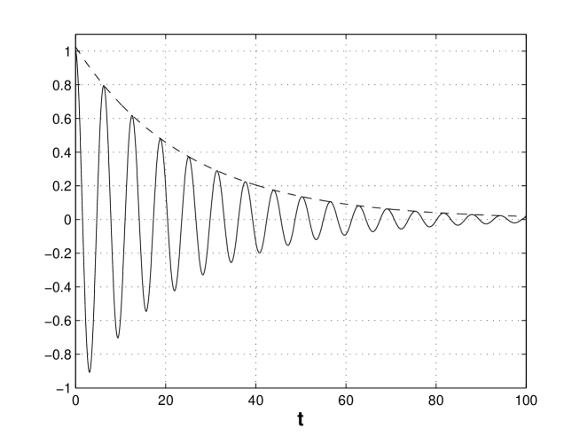
Figure 1: Rate decay of the linear fractional oscillation with initial conditions $x(0)=1$, $x^{\prime}(0)=0$ and the index $\alpha=1.95$, $f_{1.95}(0)=-0.0256$. Solid line corresponds to the solution (18), dash-line - to the approximation (23)

As an example, consider the fractional Duffing equation

$$D^{\alpha}y-y+ay^{3}=0\,,\qquad\qquad 1<\alpha<2,$$ (25)

where $a>0$ is a constant. The steady states are: $y=0$, (unstable) and $y=\pm 1/\sqrt{a}$ (stable).

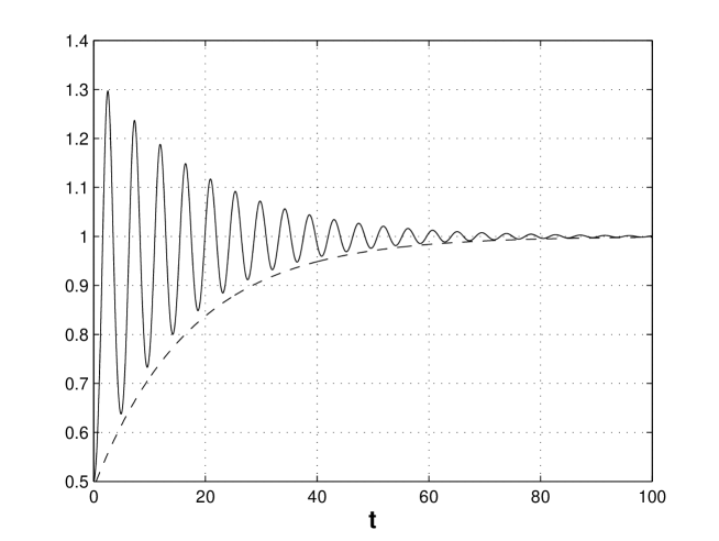
Figure 2: Rate decay of nonlinear oscillations described by the fractional Duffing equation with initial conditions $x(0)=0.5$, $x^{\prime}(0)=0$ and the index $\alpha=1.95$. The solid line is a numerical solution of (25), the dashed line is the envelope curve according to (29).

Consider Eq. (25) near a stable fixed point by the change $y\to w+1/\sqrt{a}$. Then

$$D^{\alpha}w+2w+3\sqrt{a}w^{2}+aw^{3}=0\,.$$ (26)

Close to the stable fixed point we have a linear equation

$$D^{\alpha}w_{0}+2w_{0}=0$$ (27)

with a solution

$$w_{0}(t)=BE_{\alpha}(-2t^{\alpha})\,,$$ (28)

and $B$ is a constant. For $\alpha=2-\varepsilon$ and $\varepsilon\ll 1$ expression (28) is well approximated by the relation

$$w_{0}(t)\approx\frac{2B}{2-\varepsilon}e^{\,-\sqrt{2}\gamma t}\cos(\sqrt{2}\,t)+\mathit{O}(\varepsilon^{2}).$$ (29)

with $\gamma$ from (24). Fig. 2 shows a numerical simulation of Eq.(25) in comparison with the amplitude obtained from (29). The numerical analysis of Eq. (25) is based on the algorithms described in Diethelm2005 .

When $\alpha=2$, Eqs. (25) and (26) become undamped. The leading term of the frequency of the oscillation $w$ is $\omega_{0}=2^{1/\alpha}$. From Landau , a nonlinear correction to this frequency is

$$\omega_{1}=-\frac{3\,aB^{2}}{2\sqrt{2}}<0,$$ (30)

when $aB^{2}\ll 1$, i.e. $|\omega_{1}|\ll\omega$.

From Eq. (29), we can present $w$ in the form

$$w(t)\approx w_{1}(t)+\delta w(t)=Be^{-\sqrt{2}\gamma t}\cos\Bigl{[}(\omega_{0}+\omega_{1})t+\beta\Bigr{]}+\delta w(t)\ ,$$ (31)

where $\beta$ is constant and $\delta w(t)$ is a correction to $\omega_{1}(t)$ due to the term $f_{\alpha}(t)$ in (22) that describes the polynomial decay of oscillations for fairly large $t$.

Concluding this section one state that the fractional generalization of the considered nonlinear oscillations is reduced to some effective decay of the oscillations similarly to the fractional linear oscillator. The rates of the decay can be estimated and, roughly speaking, the larger is the deviation $\varepsilon=2-\alpha$, the stronger is the decay.

IV Fractional Chaotic Attractor (FCA)

It is well known that periodic force applied to a nonlinear oscillator, for general situation, leads to the Hamiltonian chaotic dynamics in some part of phase space, while the same problem with dissipation can lead to the chaotic attractor. One can expect that the periodically perturbed fractional nonlinear oscillator should display a kind of chaos that we call FCA. Description of this phenomenon is the subject of this section. The basic equation is

$$D^{\alpha}x-x+x^{3}=F\sin(\nu t)\,,\qquad\qquad 1<\alpha<2,$$ (32)

where $F$ and $\nu$ are parameters of the perturbation. For fairly small $\varepsilon=2-\alpha$, let us introduce a cojoint equation

$$\ddot{x}+a_{1}\dot{x}-x+x^{3}=F_{1}\sin(\nu_{1}t)\ \ .\$$ (33)

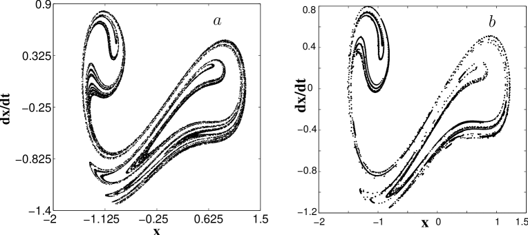
Figure 3: Poincar$\acute{\rm e}$ maps: (a) for the ordinary Duffing equation driven by periodic force: $a_{1}=0.1172$, $F_{1}=0.279$, $\nu_{1}=1.0149$; (b) for the fractional Duffing equation with the index $\alpha=1.9$, $\nu=1$, $F=0.3$, $t_{max}=16\pi$, driven by periodic force. Number of trajectories in (b) is 2000.

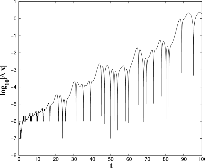
Figure 4: Exponential growth of distance $|\Delta x|$ of initially close trajectories ($\Delta x=10^{-6}$, $t=0$) for the FCA. $F=0.3$; $\nu=1$.

Simulation of Eq. (33) shows a typical chaotic attractor in Fig. 3,(a). One can recalculate the value of $\alpha$ into a corresponding $a_{1}$. As a result, in Fig. 3,(b) we see the map of the FCA. These figures display a structural difference between CA and FCA. We can assume that for small $\varepsilon$ and up to the terms of $\varepsilon^{2}$ the behavior of the FCA is similar to the CA of the cojoint equation. Nevertheless, it seems that this similarity is not complete and some strong difference is indicated below.

The computational time for Eq. (32) is very large in order to keep a reasonable accuracy. To reduce this time one can consider a short time of computation but with large number of trajectories . That is a way how the Fig. 3,(b) was obtained. It means that the Poincaré maps for CA and FCA were obtained in different ways. To check the presence of chaotic dynamics, we consider growth of the distance $|\Delta x|$ for two initially close trajectories for Eq. (32). This result is in Fig. 4 and it conforms the presence of a positive Lyapunov exponent. Nevertheless, we can see almost regular returns of $|\Delta x|$ to the initial value $10^{-6}$.

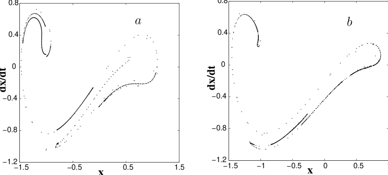
Figure 5: Reduction of structures for the FCA with the growth of $\varepsilon=2-\alpha$: (a) $\alpha=1.82$, $\nu=0.985$, $F=0.39$; (b) $\alpha=1.7$, $\nu=0.955$, $F=0.6$. Number of trajectories is 200.

As it was mentioned above, increase of the “fractionality” of the the derivative order $\varepsilon=2-\alpha$ can increase the dissipation. This leads to some “reduction of structures” in the FCA (see Fig. 5) similarly to the case of CA Zaslavsky1978 .

Finally, we present the case of a “dying attractor” Zaslavsky1978 in Fig. 6. Although the phase portrait looks very regularly, the dispersion of initially close trajectory shows randomness with the most probably zero Lyapunov exponent. This case can be related to the fractional pseudochaotic attractor (FPCA) that has a counterpart (pseudochaos) in Hamiltonian dynamics rz11 . Two comments support this hypothesis: (a) there is no separation of the initially close trajectories for fairly large time after which the distance jumped to the order one (see Fig. 6,(b)); (b) there is no structure of the attractor in Fig. 6,(a) even when we strongly increase a resolution of the Poincaré section plot, i.e. the dimension of the set in Fig. 6,(a) is rather one than larger of one as in Fig. 3,(a).

Figure 6: Dying FCA: $\alpha=1.82$, $F=0.3$, $\nu=1$; (a) phase plane of the FCA; (b) dispersion of initially close two trajectories.

V Conclusions

Since the fractional derivatives are time-directed, the equations with fractional derivatives slightly different from the integer ones by $\varepsilon=2-\alpha\ll 1$ can be fairly easy interpreted through the regular equations with a dissipation. As a result, fractional nonlinear oscillator behaves like the stochastic attractor in phase space, being periodically perturbed. The role of the polynomial dissipation is still elusive. It seems that this term leads to a degradation of the FCA structure. The error has fast increase with time creating difficulties in the simulations (see Fig. 7). Due to that we can not provide explicit features of the difference between CA and FCA.

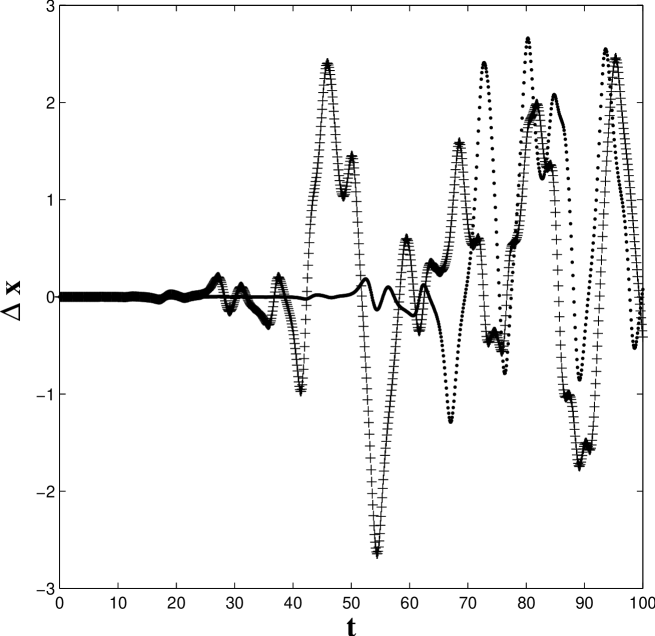
Figure 7: Errors between the numerical calculations with time steps 0.01 and 0.001 (dots); with time steps 0.001 and 0.1 (pluses) .

The resonant case for the linear oscillator can be interpreted in the way similar to the integer derivative case with $\alpha=2$ Landau (see Appendix 2). Our simulations show that applying the fractional calculus, one can gain a compact formulations of dynamics with new properties governed by a complexity of the media.

Appendix 1

Here we consider a presentation of the solution to equation (17). Two independent solutions are

$$e_{\alpha}(t)=E_{\alpha,\,1}(-t^{\alpha})\,,\qquad i_{\alpha}(t)=t^{\alpha/2}E_{\alpha,\,1+\alpha/2}(-t^{\alpha})\,.$$ (34)

Let $u(t)$ be a function and $L.T.u(t)$ be its Laplace transform, namely

$$L.T.u(t)=u(s)=\int_{0}^{\infty}e^{-st}\,u(t)\,dt.$$ (35)

Then the Laplace transforms of $e_{\alpha}(t)$ and $i_{\alpha}(t)$ become

$$L.T.e_{\alpha}(t)=\frac{s^{\alpha-1}}{s^{\alpha}+1}\ ;\ \ \ \ \qquad L.T.i_{\alpha}(t)=\frac{s^{-1+\alpha/2}}{s^{\alpha}+1}\,.$$ (36)

Let us deform the Bromwich path of integration into the equivalent Hankel path. Then the loop starts from minus infinity along the lower side of negative real axis, encircles $|s|=1$ counter-clockwise and ends at minus infinity along the upper side of the negative real axis. This allows one to decompose the functions $e_{\alpha}(t)$ and $i_{\alpha}(t)$ into two terms. The first contribution arises from two borders of the cut along the negative real semi-axis. The second contribution is determined by residues in the poles $s_{0}=\exp(j\pi/\alpha)$ and $s_{1}=\exp(-j\pi/\alpha)$. We arrive to the expressions (19)-(20) Gorenflo for the function $e_{\alpha}(t)$. Similarly, we can present

$$i_{\alpha}(t)=h_{\alpha}(t)+q_{\alpha}(t)\,,$$ (37)

where

$$h_{\alpha}(t)=\frac{1}{\pi}\int_{0}^{\infty}e^{-\,rt}\,\frac{r^{-1+\alpha/2}(1-r^{\alpha})\sin(\pi\alpha/2)\,dr}{r^{2\alpha}+2r^{\alpha}\cos(\pi\alpha)+1}\,,$$ (38)

$$q_{\alpha}(t)=\frac{2}{\alpha}\,e^{\,t\cos(\pi/\alpha)}\sin\left[t\sin\Bigl{(}\frac{\pi}{\alpha}\Bigr{)}\right].$$

For the detailed analysis of these expressions see StanislavskyPHYSA05 .

Appendix 2 Driven linear fractional oscillator

In this section we discuss briefly some features of linear fractional oscillator perturbed by an analog of the resonant external force (see also Achar ). “Free” and “forced” oscillations of the fractional oscillator depend on the index $\alpha$. The main conclusion is that the dynamical response of the driven fractional oscillator is bounded in amplitude for any relation between the oscillator frequency and the frequency of the perturbation. The finiteness of the response indicates a damped character of fractional derivative. In StanislavskyPRE04 the linear fractional oscillator is interpreted as an ensemble average over harmonic oscillations because of the interaction of the fractional system with the random environment. The intrinsic absorption of the fractional oscillator results from the response of each harmonic oscillator being compensated by an antiphase response of another harmonic oscillator (see details in StanislavskyPRE04 ). This shows the main difference between the resonant phenomenon in regular systems and the resonance in fractional systems (both linear and nonlinear).

Let the external force in the linear fractional oscillator equation be described by Mittag-Leffler function

$$D^{\alpha}x+\omega^{2}_{0}x=CE_{\alpha}(-\omega^{2}t^{\alpha})\ ,\qquad\qquad 1<\alpha<2\,,$$ (39)

where $C$ is a constant determined by initial conditions. Since the equation is linear, its solution can be presented in the form similar to Landau

$$x(t)=A_{1}E_{\alpha}(-\omega_{0}^{2}t^{\alpha})+\frac{C_{1}}{\omega^{2}_{0}-\omega^{2}}\left[E_{\alpha}(-\omega^{2}t^{\alpha})-E_{\alpha}(-\omega^{2}_{0}t^{\alpha})\right]\,,$$ (40)

where $A_{1}$, $C_{1}$ are new constants. A direct calculation gives

$$\lim_{\omega\to\omega_{0}}x(t)=A_{1}E_{\alpha}(-\omega_{0}^{2}t^{\alpha})+C_{1}\frac{t^{\alpha}}{\alpha}\,E_{\alpha,\,\alpha}(-\omega_{0}^{2}t^{\alpha})\,.$$ (41)

For $t\to 0$ the second term tends to zero. For $1<\alpha<2$, $t\gg 1$ we have

$$t^{\alpha}E_{\alpha,\,\alpha}(-\omega^{2}_{0}t^{\alpha})\sim\frac{t^{-\alpha}}{\omega^{4}_{0}\Gamma(1-\alpha)}\,,$$ (42)

and the same is for the first term of (41)

$$E_{\alpha}(-\omega_{0}^{2}t^{\alpha})\sim\frac{t^{-\alpha}}{\omega^{2}_{0}\Gamma(1-\alpha)}\,,\quad t\gg 1\,.$$ (43)

Thus, the secular term is absent for $1<\alpha<2$.

The resonance is observed only for $\alpha=2$, when Eq. (41) is transformed into the usual forced harmonic oscillator. Then, the secular term appears

$$\lim_{\omega\to\omega_{0}}x_{\alpha=2}(t) = A_{1}E_{2}(-\omega_{0}^{2}t^{2})+C_{1}t^{2}E_{2,\,2}(-\omega_{0}^{2}t^{2})$$ (44)

$$= A_{1}\cos\omega_{0}t+\frac{C_{1}t}{2\omega_{0}}\sin\omega_{0}t\,.$$

Concluding, the linear fractional oscillator forced by a Mittag-Leffler oscillation does not go to any resonance for $\omega\to\omega_{0}$ for $1<\alpha<2$.

References

- (1) E. Ott, “Chaos in dynamical systems”, Cambridge University Press, New York, 1993.
- (2) G. M. Zaslavsky, Phys. Lett. A, 69, 145-147 (1978).
- (3) K. T. Alligood, T. D. Sauer, J. A. Yorke, “CHAOS: An introduction to dynamical systems”, Springer-Verlag, New York, 1996.
- (4) G. M. Zaslavsky, Physica D, 76, 110-122 (1994); Chaos, 4, 25-33 (1994).
- (5) G. M. Zaslavsky, Phys. Reports, 371, 461 (2002).
- (6) A. Piryatinska, A. I. Saichev, W. A. Woyczynski, Physica A, 349, 375-420 (2005).
- (7) T. L. Szabo, J. Acoust. Soc. of Am., 96, 491 (1994); D. T. Blackstock, ibid. 77, 2050 (1985); W. Chen, S. Holm, ibid. 115, 1424 (2004).
- (8) R. R. Nigmatullin, Phys. Sta. Sol. (b), 133, 425 (1986).
- (9) T. F. Nonnenmacher, In “Lecture Notes in Physics”, v. 381, p. 309, Springer, Berlin, 1991.
- (10) H. Weitzner, G. M. Zaslavsky, Commun. Nonlin. Sci. and Numer. Simul., 8, 273-281 (2003).
- (11) N. Laskin, Phys.Rev. E, 66, 056108 (2002).
- (12) E. Goldfain, Chaos, Solitons and Fractals, 19, 1023-1030 (2004); 22, 513-520 (2004); 23, 701-710 (2005).
- (13) I. M. Gelfand, G. E. Shilov, “Generalized Functions I: Properties and Operations”, Academic, New York, 1964.
- (14) S. G. Samko, A. A. Kilbas, O. I. Marichev, “Fractional Integrals and Derivatives and Some of Their Applications”, Nauka i Technika, Minsk (1987) (in Russian).
- (15) M. M. Meerschaert, D. A. Benson, H. P. Scheffler, B. Baeumer, Phys.Rev. E, 66, 060102 (2002).
- (16) I. Podlubny, “Fractional Differential Equations”, Academic Press, New York, 1999.
- (17) K. S. Miller, B. Ross, “An Introduction to the Fractional Calculus and Fractional Differential Equations”, Wiley, New York, 1993.
- (18) A. I. Saichev and G. M. Zaslavsky, Chaos, 7, 753-764 (1997).
- (19) V. V. Uchaikin, V. M. Zolotarev, “Chance and Stability. Stable Distributions and their Applications”, VSP, Utrecht (1999).
- (20) A. A. Stanislavsky, Theor. and Math. Phys., 138, 418-431 (2004).
- (21) F. Mainardi, Chaos, Soliton & Fractals, 7, 1461-1477 (1996).
- (22) R. Gorenflo, F. Mainardi, In Proceedings of the International Workshop on the Recent Advances in Applied Mathematics (RAAM ’96), Kuwait, 1996, Kuwait University, Department of Mathematics and Computer Science, pp. 193-208.
- (23) M. Seredyska, A. Hanyga, J. Math. Phys., 41, (2135-2156 (2000).
- (24) A. A. Stanislavsky, Phys.Rev. E, 70, 051103 (2004).
- (25) M. D. Ortigueria, Signal Processing, 83, 2301 (2003).
- (26) Yu. Rabotnov, “Creep problems in structural members”, North-Holland, Amsterdam, 1969, p. 129. Originally published in Russian as: Polzuchest’ Elementov Konstruktsii, Nauka, Moscow, 1966.
- (27) M. Caputo, J. Roy. Astron. Soc., 13, 529-539 (1967).
- (28) A. Erdlyi, “Higher Transcendental Finctions”, Vol. III, Sec. 18, McGraw-Hill, New York, 1955.
-
(29)
A. Chatterjee, Nonlinear Dyn., 32,
323-343 (2003);
P. Wahi, A. Chatterjee, Nonlinear Dyn., 38, 3-22 (2004). - (30) A. A. Stanislavsky, Physica A, 354, 101-110 (2005).
- (31) K. Diethelm, N. J. Ford, A. D. Freed, Yu. Luchko, Comput. Methods Appl. Mech. Engrg., 194, 743-773 (2005).
- (32) L. D. Landau, E. M. Lifschitz, “Mechanics”, 3rd ed., Pergamon Press, Oxford, England, 1976.
- (33) O. Lyubomudrov, M. Edelman, G. M. Zaslavsky, Int. J. Mod. Phys. B, 17, 4149 (2003); G. M. Zaslavsky, M. Edelman, Physica D, 193, 128-147 (2004).
- (34) B. N. Narahari Achar, J. W. Hanneken, T. Clarke, Physica A, 309, 275-288 (2002); B. N. Narahari Achar, J. W. Hanneken, T. Clarke, Physica A, 339, 311-319, (2004).