Fractal Stationary Density in Coupled Maps

Abstract

We study the invariant measure or the stationary density of a coupled discrete dynamical system as a function of the coupling parameter $\epsilon$ ($0<\epsilon<1/4$). The dynamical system considered is chaotic and unsynchronized for this range of parameter values. We find that the stationary density, restricted on the synchronization manifold, is a fractal function. We find the lower bound on the fractal dimension of the graph of this function and show that it changes continuously with the coupling parameter.

1 Introduction

Two or more coupled rhythms can under certain conditions synchronize, that is a definite relationship can develop between these rhythms. This phenomena of synchronization PRK ; Pecora1997 in coupled dynamical systems has acquired immense importance in recent years since it appears in natural phenomena as well as in engineering applications. What is even more interesting is the fact that even chaotic oscillations can synchronize. This observation is being utilized in secure communication VanWiggeren1998 . Studying synchronization is also important for neural information processing  Hansel1992 ; Buzsaki2004 ; Friedrich2004 .

These developments have lead to the investigation of coupled dynamical systems. The dynamical systems considered can either be continuous or discrete in time. Different types of couplings have been considered, like continuously coupled or pulsed coupled. And many coupling topologies arise in nature as well as in human applications, like random, all-to-all, scale-free, small-world, nearest neighbour lattice, etc. Also the coupling strengths can vary from element to element. We plan to study a system of two coupled maps which forms a basic building block of all these systems and allows us to separate the complexity due to coupling topologies from that coming from the chaotic nature of the dynamical system considered. As a next step, one can then consider various coupling topologies. We have demonstrated in Jost2004 that the result of such a system of two coupled maps can be used to derive the result for a globally coupled network of $N$ maps. Here we are concerned with the phenomena of complete synchronization, that is, the dynamics of two systems becomes completely identical after the coupling parameter crosses a certain critical value.

The model

We consider the following coupled map system

$$X_{n+1}=AF(X_{n}):=S(X_{n})$$ (1)

where $X=(x,y)^{T}$ is a 2-dim column vector, $A$ is a $2\times 2$ coupling matrix and $F$ is a map from $\Omega=[0,1]\times[0,1]$ onto itself. In the present paper we take $F$ to be the extension of the tent map $f_{t}:[0,1]\rightarrow[0,1]$,

$$f_{t}(x)=\left\{\begin{array}[]{lcl}2x&&0\leq x\leq 1/2\\ 2-2x&&1/2\leq x\leq 1\end{array}\right.,$$ (4)

to two variables and we choose

$$A=\left(\begin{array}[]{cc}1-\epsilon&\epsilon\\ \epsilon&1-\epsilon\end{array}\right)$$ (7)

where $0<\epsilon<1$ is the coupling strength. This type of coupling has been called contractive or dissipative. See PRK for the physical motivation behind considering such a system. Furthermore, the row sums of $A$ are equal to one which guarantees the existence of a synchronized solution.

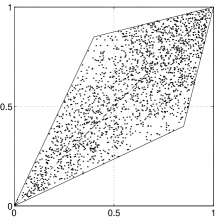
Figure 1: Asymptotic distribution of 2000 points starting from an uniform distribution over the whole phase space $\Omega$. $\epsilon=0.2$.

Before proceeding we give a mathematical definition of synchronization we are interested in.

Definition 1

A discrete dynamical system $S:\Omega\rightarrow\Omega$ is said to completely synchronize if as $n$ tends to infinity $|S^{n}(x)-S^{n}(y)|$ tends to zero for all $(x,y)\in\Omega$.

Using the linear stability analysis it can be shown jost2002 that this coupled map system synchronizes when $1/4<\epsilon<3/4$. The same result was also obtained by studying the evolution of the support of the invariant measure Jost2004 which is a global result as opposed to the linear stability analysis which is carried out near the synchronized solution. This was done by showing that if $\epsilon<1/4$ we obtain a quadrilateral of nonzero area as the support of the invariant measure. We depict this area in Fig 1 along with a distribution of points obtained from uniform distribution of initial conditions. And when $\epsilon$ crosses the value 1/4 this quadrilateral shrinks to the line $x=y$. In this sense the synchronization transition is a discontinuous transition.

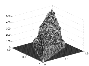
Figure 2: The stationary density: a histogram of the distribution of points of Fig. 1. Here the number of point is $10^{6}$ and the mesh size is 100x100. The horizontal plane depicts $\Omega$ and the vertical axis gives the number of points lying in the mesh square.

But this figure is misleading as it does not tell us anything about the density of points. As we show in Fig. 2, if we plot the histogram then we see a quite irregular structure. In Fig. 3 we plot the section of this invariant density along the line $x=y$. We see clearly that it is an irregular function. Studying this invariant density is the object of this paper. In particular we show that this density is indeed a fractal function on the synchronization manifold, i.e., its section along line $x=y$, and the fractal dimension of the graph of this function depends on the coupling parameter.

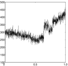
Figure 3: The section of the stationary density along the line $x=y$. In this graph the total number of points used is $10^{8}$ and the size of the mesh used is 1000x1000.

The paper is organized as follows. In section 2 we give a brief introduction to invariant measures recalling some definitions and results required for completeness. We also outline a method to find the stationary density. We then move on to our main result in the section 3 after introducing basic concepts needed to characterize the irregularity of fractal functions. Section 4 concludes by pointing out some future directions.

2 Invariant measure

Invariant measures or the stationary densities LM provide a useful way to study the asymptotic behavior of dynamical systems. One starts with a distribution of initial conditions and studies its evolution as time goes to infinity. It is interesting to note that even if the dynamical system is chaotic a well behaved limit can exist which can then be used to study various average properties. In this section we give a brief introduction to invariant measures and a way to find one. We begin with the definitions (the norms used are $L^{1}$ norms throughout):

Definition 2

A measure $\mu$ is said to be invariant under a transformation $S$ if $\mu(S^{-1}(A))=\mu(A)$ for any measurable subset $A$ of $\Omega$.

Definition 3

Let $(X,A,\mu)$ be a measure space and the set $D(X,A,\mu)$ be defined by $D(X,A,\mu)=\{f\in L^{1}(X,A,\mu):f\geq 0\mbox{ and }||f||=1\}$. Any function $f\in D(X,A,\mu)$ is called a density.

Definition 4

Let $(X,A,\mu)$ be a measure space. A linear operator $P:L^{1}\rightarrow L^{1}$ satisfying

(a) $Pf\geq 0$ for $f\geq 0$, $f\in L^{1}$; and

(b) $||Pf||=||f||$, for $f\geq 0$, $f\in L^{1}$

is called a Markov operator.

A Markov operator satisfies a contractive property, viz., $||Pf||\leq||f||$. And this property implies the stability property of iterates of Markov operators, viz., $||Pf-Pg||\leq||f-g||$. We shall be interested in the fixed points of Markov operators.

Definition 5

Let $(X,A,\mu)$ be a measure space and $P$ be a Markov operator. Any $f\in D$ that satisfies $Pf=f$ is called a stationary density of $P$.

A stationary density is the Radon-Nikodym derivative of an invariant measure with respect to $\mu$.

2.1 The Frobenius-Perron operator

There exist various methods to find invariant measures. One approach is to use the so called Frobenius-Perron operator. This operator when applied to $\rho_{n}(x)$, the density at the $n$th time step, yields the density at the $(n+1)$th time step. Since all the points at the $(n+1)$th step in some set $D$ come from the points in the set $S^{-1}(D)$ we have the following equality defining the Frobenius-Perron operator $P$:

$$\int\int_{D}P\rho(x)\mu(dx)=\int\int_{S^{-1}(D)}\rho(x)\mu(dx)$$ (8)

The Frobenius-Perron operator is a Markov operator.

2.2 The invariant measure of the tent map

If in (8) we choose our discrete dynamical system to be the one dimensional tent map defined in (4) and $D=[0,x]$ then the equation (8) reduces to

$$P\rho(x)=\rho(x/2)+\rho(1-x/2).$$ (9)

We are interested in the fixed point solutions; this leads to

$$\rho(x)=\rho(x/2)+\rho(1-x/2).$$ (10)

A solution of this functional equation is $\rho(x)=1$. Of course, this is a trivial solution. $\delta(x)$ and $\delta(x-2/3)$ also solve this equation but we are not interested in such singular solutions since they do not span the phase space.

3 Stationary density of the coupled tent map

We now turn to coupled maps. In this section we study the stationary density on the synchronization manifold, i.e., the line $x=y$. We show that the density is a fractal function with its Hölder exponent related to the coupling parameter $\epsilon$.

We use the following definition of Hölder continuity and its relation to the box dimension falconer1990 :

Definition 6

A function $f:[0,1]\rightarrow R$ is in $C_{x_{0}}^{\alpha}$, for $0<\alpha<1$ and $x_{0}\in[0,1]$, if for all $x\in[0,1]$

$$|f(x)-f(x_{0})|\leq c|x-x_{0}|^{\alpha}.$$ (11)

A pointwise Hölder exponent $\alpha_{p}(x_{0})$ at $x_{0}$ is the supremum of the $\alpha$s for which the inequality (11) holds. We also use the relation between the Hölder continuity and the box dimension of the graph a function, ${\rm dim_{B}graph}f$.

Proposition 1

If for $f:[0,1]\rightarrow R$, the pointwise Hölder exponent is $\alpha$ for all $x\in[0,1]$ and $c$ in (11) is uniform then ${\rm dim_{B}graph}f=2-\alpha$.

Now we are ready to state and prove our main result, viz, the estimate of the box dimension of the graph of the stationary density.

Theorem 3.1

Let $\rho(x,y)$ be the stationary density of the coupled dynamical system (1) and let $\rho^{D}(x)$ be its restriction on the line $x=y$. If $\rho(x,y)$ is bounded then ${\rm dim_{B}graph}\rho^{D}\geq d$ where $d=2+\ln(1-2\epsilon)/\ln 2$, with $0<\epsilon\leq 1/4$.

Proof: We use the Frobenius-Perron operator defined in equation (8). We choose $D=[0,x]\times[0,y]$ and get

$$P\rho(x,y)={\partial\over\partial x}{\partial\over\partial y}\int\int_{S^{-1}(D)}\rho(x^{\prime},y^{\prime})dx^{\prime}dy^{\prime}$$ (12)

Our $S$ in equation (1) is not invertible. In fact, it has 4 preimages. Let us denote them by $S_{i}^{-1}$, $i=1,...,4$. If $X\in\Omega$, since $f$ is symmetric, we get

$$P\rho(X)=J^{-1}(X)\sum_{i=1}^{4}\rho(S_{i}^{-1}(X))$$ (13)

where $J^{-1}(X)=|dS^{-1}(X)/dX|$. The fixed point of this operator is given by the following functional equation for the density.

$$\rho(x,y) = {1\over{4|1-2\epsilon|}}[\rho(\beta x/2-\gamma y/2,-\gamma x/2+\beta y/2)$$ (14)

$$+\rho(1-\beta x/2+\gamma y/2,-\gamma x/2+\beta y/2)$$

$$+\rho(\beta x/2-\gamma y/2,1+\gamma x/2-\beta y/2)$$

$$+\rho(1-\beta x/2+\gamma y/2,1+\gamma x/2-\beta y/2)]$$

where $\gamma=\epsilon/1-2\epsilon$ and $\beta=1+\gamma$. Since we know that a point belonging to $\Omega$ does not leave $\Omega$, all the arguments of $\rho$ on the right hand side of the above equation should be between 0 and 1. This gives us four lines which bound an area $0\leq\beta x/2-\gamma y/2\leq 1$ and $0\leq-\gamma x/2+\beta y/2\leq 1$. Lets denote this area by $Gamma$. The support of the invariant measure should be contained in $\Gamma\cap\Omega$.

We also remark that for $0\leq\epsilon<1/4$, the discrete dynamical system $S$ that we have considered is everywhere expanding and this implies that the stationary density exists LM .

The above equation can be written as, for $0\leq\epsilon<1/4$,

$$\rho(x,y)={1\over{(1-2\epsilon)}}\rho_{SS}(\beta x/2-\gamma y/2,-\gamma x/2+\beta y/2)$$ (15)

where

$$\rho_{SS}(x,y)={{\rho(x,y)+\rho(1-x,y)+\rho(x,1-y)+\rho(1-x,1-y)}\over 4}$$ (16)

is the part of $\rho$ that is symmetric around $1/2$ in both arguments. Now if we substitute $x=y$ in equation (15) we see that the arguments on both sides of the equation belong to the diagonal. As a result we obtain a functional equation

$$\rho^{D}(x)={1\over{(1-2\epsilon)}}\rho^{D}_{S}(x/2)$$ (17)

where we use a shorthand notation $\rho^{D}_{S}(x)=\rho^{D}_{SS}(x,x)$. With the change of variable $z=x/2$ and a decomposition of $\rho^{D}(x)$ as $\rho^{D}(x)=\rho^{D}_{S}(x)+\rho^{D}_{A}(x)$, the ”symmetric” and ”antisymmetric” part where again $\rho^{D}_{A}(x)$ is a shorthand notation for $\rho^{D}_{AS}(x,x)+\rho^{D}_{SA}(x,x)+\rho^{D}_{AA}(x,x)$ , we arrive at

$$\rho^{D}_{S}(z)=(1-2\epsilon)\rho^{D}_{S}(2z)+g(z)$$ (18)

where $g(z)=(1-2\epsilon)\rho^{D}_{A}(2z)$. Its solution can be written down as

$$\rho^{D}_{S}(z)=\sum_{k=0}^{\infty}(1-2\epsilon)^{k}g(2^{k}z).$$ (19)

This is a Weierstrass function and if $g(z)\in C^{\beta}$ where $\beta>-\ln(1-2\epsilon)/\ln 2$ then the calculation in falconer1990 for $g(z)=\sin(z)$ can be carried over and it can be shown that the pointwise Hölder exponent of this function is $-\ln(1-2\epsilon)/\ln 2$ everywhere implying that ${\rm dim_{B}graph}\rho^{D}_{S}=d$. And if $g(z)$ is not smooth enough then it can only increase the box dimension of $\rho^{D}(x)$, hence the result. ∎

4 Concluding Remarks

We have studied the stationary density of two coupled tent maps as a function of the coupling parameter. We find that even though the density of the individual tent map is smooth it becomes very irregular as soon as a small coupling is introduced in the sense that the pointwise Hölder exponent is small everywhere. And the density smoothes as the coupling is increased. It becomes smooth that is the Hölder exponent becomes one at the value of $\epsilon$ where the synchronization transition takes place. We have thus elucidated a new aspect of synchronization in coupled dynamical systems, beyond the standard aspects of linear or global stability of synchronized solutions.

It is a curious fact that the Hölder exponent becomes one exactly at the critical value of the coupling parameter, i.e., $\epsilon_{c}=1/4$. It would be important to understand if there is any underlying principle behind this observation, that is, one valid also for other maps with varying coupling matrices.

It is interesting to note that fractal probability densities have arisen in a completely different scenario, namely the random walk problem with shrinking step lengths Krapivsky2004 .

One should also characterize the stationary density away from the synchronization manifold. It is expected to have a more complex multifractal character Jaffard1997 . The effect of different network topologies on the stationary density is another interesting topic.

One of us (KMK) would like to thank the Alexander-von-Humboldt-Stiftung for financial support.

References

- [1] A. Pikovsky, M. Rosenblum, and J. Kurths. Synchronization - A Universal Concept in Nonlinear Science. Cambridge University Press, 2001.
- [2] L. M. Pecora, T. L. Carroll, G. A. Johnson, D. J. Mar, and J. F. Heagy. Fundamentals of synchronization in chaotic systems, concepts, and applications. Chaos, 7:520, 1997.
- [3] G. D. VanWiggeren and R. Roy. Communication with chaotic lasers. Science, 279:1198, 1998.
- [4] D. Hansel and H. Sompolinsky. Synchronization and computation in a chaotic neural network. Phys. Rev. Lett., 68:718, 1992.
- [5] G. Buzsáki and A. Draguhn. Neuronal oscillations in cortical networks. Science, 304:1926, 2004.
- [6] R. W. Friedrich, C. J. Habermann, and G. Laurent. Multiplexing using synchrony in the zebrafish olfactory bulb. Nature Neuroscience, 7:862, 2004.
- [7] J. Jost and K. M. Kolwankar. Global analysis of synchronization in coupled maps, 2004.
- [8] J. Jost and M. P. Joy. Spectral properties and synchronization in coupled map lattices. Phys. Rev. E, 65(1):016201, 2002.
- [9] A. Lasota and M. C. Mackey. Chaos, Fractals and Noise. Springer, 1994.
- [10] K. Falconer. Fractal Geometry - Mathematical Foundations and Applications. John Wiley, 1990.
- [11] P. L. Krapivsky and S. Redner. Random walk with shrinking steps. Am. J. Phys., 72:591, 2004.
- [12] S. Jaffard. Multifractal formalism for functions part ii: Self-similar functions. SIAM J. Math. Anal., 28:971, 1997.