One of the fourth-order analog to the first Painlevé equation is studied. All power expansions for solutions of this equation near points $z=0$ and $z=\infty$ are found by means of the power geometry method. The exponential additions to the expansion of solution near $z=\infty$ are computed. The obtained results confirm the hypothesis that the fourth-order analog of the first Painlevé equation determines new transcendental functions.

1 ​​​​​​.   Introduction.

More than one century ago Painlevé and his school discovered six irreducible second-order equations, which determine new transcendental functions. Over a long period of time these functions seemed to have no physical applications, but now these equations are widely used for description of different physical processes. At the present the problem of analysis of the higher analogs to the Painlevé equations has appeared. There is a lot of works, devoted to the solution of this problem [1, 2, 3, 4, 5, 6, 7, 8, 9, 10, 11, 12, 13]. One of the fourth-order analogs of the first Painlevé equation is equation

$$w_{zzzz}+18w\,w_{zz}+9w^{2}_{z}+24w^{3}=z$$ (1.1)

In papers [3, 14, 2, 15, 16, 9] it was shown that equation (1.1) has properties, that are typical for the Painlevé equations $P_{1}\div P_{6}$. Equation (1.1) belongs to the class of exactly solvable equations, as it has Lax pair and a lot of other typical properties of the exactly solvable equations. However it does not have the first integrals in the polynomial form, that is one of the features of the Painlevé equations. Equation (1.1) seems to determine new transcendental functions just as equations $P_{1}\div P_{6}$, although the rigorous proof of the irreducibility of equation (1.1) is now the open problem.

Thereupon the study of all the asymptotic forms and power expansions of equation (1.1) is the important stage of the analysis of this equation, as this fact indirectly confirms the irreducibility of equation (1.1).

This equation does not have the exact solutions, and so it is very important to find the asymptotic forms and the power expansions of the solution of this equation, that is the aim of this work.

Let us find all the power expansions for the solution of equation (1.1) in the form of

$$w(z)=c_{r}\,z^{r}+\sum_{s}\,c_{s}\,z^{s}$$ (1.2)

at $z\rightarrow\,0$, then $\omega=-1$, $s>r$ and at $z\rightarrow\,\infty$, then $\omega=1$, $s<r$.

For that we use the power geometry method [17, 18, 19, 20].

The outline of this paper is as follows. Section 2 is devoted to the general properties of equation (1.1). In sections 3–5 the expansions near $z=0$ are found. In sections 6–9 the power expansion near $z=\infty$ and its exponential additions are obtained.

2 ​​​​​​.  The general properties of equation (1.1).

Let us consider the fourth-order equation (1.1)

$$f(z,w)\stackrel{{\scriptstyle def}}{{=}}w_{zzzz}+18ww_{zz}+9w^{2}_{z}+24w^{3}-z=0$$ (2.1)

For monomials of equation (2.1) we have points $M_{1}=(-4,1),\,\,\,M_{2}=(-2,2),\,\,\,M_{3}=(-2,2),\,\,\,M_{4}=(0,3),\,\,\,M_{5}=(1,0)$.

The carrier of equation is defined by four points $Q_{1}=M_{1}$, $Q_{2}=M_{4}$, $Q_{3}=M_{5}$ and $Q_{4}=M_{2}=M_{3}$. Their convex hull $\Gamma$ is the triangle (fig. 1).

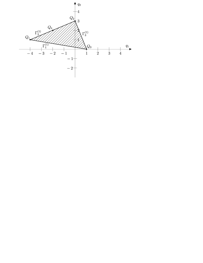
Figure 1:

This triangle has apexes $Q_{j}\,(j=1,2,3)$ and edges $\Gamma_{1}^{(1)}=[Q_{3},\,Q_{1}],\,\,\Gamma_{2}^{(1)}=[Q_{1},\,Q_{2}],\,\,\Gamma_{3}^{(1)}=[Q_{2},\,Q_{3}]$

Outward normal vectors $N_{j}\,(j=1,2,3)$ of edges $\Gamma_{j}^{(1)}\,(j=1,2,3)$ are determined by vectors

$$N_{1}=(-1,-5),\,\,\,N_{2}=(-1,2),\,\,\,N_{3}=(3,1)$$ (2.2)

The normal cones $U_{j}^{(1)}$ to edges $\Gamma_{j}^{(1)}$ are

$$U_{j}^{(1)}=\mu N_{j},\,\,\,\mu>0,\,\,\,j=1,2,3$$ (2.3)

They and the normal cones $U_{j}^{(0)}$ of apexes $\Gamma_{j}^{(0)}=Q_{j}\,\,(j=1,\,2,\,3)$ are represented at fig. 2.

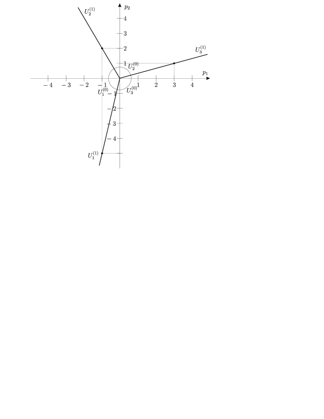
Figure 2:

We can choose the basis of the lattice of the carrier of equation (2.1) as

$$B_{1}=(-5,\,1),\,\,\quad\,B_{2}=(-3,\,2)$$ (2.4)

Let us study solutions, corresponding to the bounds $\Gamma_{j}^{(d)},\,\,d=0,1;\,\,j=1,\,2,\,3$ in view of the reduced equations, conforming to apexes $\Gamma_{j}^{(0)}(j=1,\,2,\,3)$

$$\hat{\emph{f}}_{1}^{(0)}\stackrel{{\scriptstyle def}}{{=}}w_{zzzz}=0$$ (2.5)

$$\hat{\emph{f}}_{2}^{(0)}\stackrel{{\scriptstyle def}}{{=}}24\,w^{3}=0$$ (2.6)

$$\hat{\emph{f}}_{3}^{(0)}\stackrel{{\scriptstyle def}}{{=}}\,-z=0$$ (2.7)

and reduced equations, conforming to edges $\Gamma_{j}^{(1)}(j=1,2,3)$

$$\hat{\emph{f}}_{1}^{(1)}\stackrel{{\scriptstyle def}}{{=}}w_{zzzz}-z=0$$ (2.8)

$$\hat{\emph{f}}_{2}^{(1)}\stackrel{{\scriptstyle def}}{{=}}w_{zzzz}+18\,w\,w_{zz}+9w_{z}^{2}+24w^{3}=0$$ (2.9)

$$\hat{\emph{f}}_{3}^{(1)}\stackrel{{\scriptstyle def}}{{=}}24w^{3}-z=0$$ (2.10)

Note, that the reduced equations (2.6) and (2.7) are the algebraic ones. According to [18] they do not have non-trivial power or non-power solutions.

3 ​​​​​​.   Solutions, corresponding to apex $Q_{1}$.

Apex $Q_{1}=(-4,1)$ is corresponded to reduced equation (2.5).

Let us find the reduced solutions

$$w=c_{r}z^{r},\,\,\,c_{r}\neq 0$$ (3.1)

for $\omega(1,r)\in U_{1}^{(0)}$.

Since $p_{1}<0$ in the cone $U_{1}^{(0)}$, then $\omega=-1,\,\,\,z\rightarrow 0$ and the expansions are the ascending power series of $z$. The dimension of the bound $d=0$, therefor

$$g(z,w)=w^{4}\,w^{-1}\,w_{zzzz}$$ (3.2)

We get the characteristic polynomial

$$\chi(r)\stackrel{{\scriptstyle def}}{{=}}g(z,z^{r})=r(r-1)(r-2)(r-3)$$ (3.3)

Its roots are

$$r_{1}=0,\,\,\,r_{2}=1,\,\,\,r_{3}=2,\,\,\,r_{4}=3$$ (3.4)

Let us explore all these roots.

The root $r_{1}=0$ is corresponded to vector $R=(1,0)$ and vector $\omega R\in U_{1}^{(0)}$.

We obtain the family $\mathcal{F}_{1}^{(1)}\,1$ of reduced solutions $w=c_{0}$, where $c_{0}\neq 0$ is arbitrary constant and $\omega=-1$. The first variation of equation (2.5)

$$\frac{\delta\hat{\emph{f}}_{1}^{(0)}}{\delta w}=\frac{d^{4}}{dz^{4}}$$ (3.5)

gives operator

$$\mathcal{L}(z)=\frac{d^{4}}{dz^{4}}\neq 0$$ (3.6)

Its characteristic polynomial is

$$\nu(k)=z^{4-k}\mathcal{L}(z)\,z^{k}=k(k-1)(k-2)(k-3)$$ (3.7)

Equation

$$\nu(k)=0$$ (3.8)

has four roots

$$k_{1}=0,\,\,\,k_{2}=1,\,\,\,k_{3}=2,\,\,\,k_{4}=3$$ (3.9)

As long as $\omega=-1$ and $r=0$, then the cone of the problem is

$$\mathcal{K}=\{k>0\}$$ (3.10)

It contains the critical numbers $k_{2}=1,\,\,\,k_{3}=2$ and $k_{3}=3$. Expansions for the solutions, corresponding to reduced solution (3.1) can be presented in the form

$$w=c_{0}+c_{1}z+c_{2}z^{2}+c_{3}z^{3}+\sum^{\infty}_{k=4}c_{k}z^{k}$$ (3.11)

where all the coefficients are constants, $c_{0}\neq 0,\,\,\,c_{1},\,\,\,c_{2}$, $c_{3}$ are arbitrary ones and $c_{k}\,\,(k\geq 4)$ are uniquely defined. Denote this family as $\emph{G}_{1}^{(0)}1$. Expansion (3.11) with taking into account eight terms is

$$\begin{gathered}w\left(z\right)=c_{{0}}+c_{{1}}z+c_{{2}}{z}^{2}+c_{{3}}{z}^{3}-\left(\frac{3}{2}\,c_{{0}}c_{{2}}+{c_{{0}}}^{3}+\frac{3}{8}\,{c_{{1}}}^{2}\right){z}^{4}+\\ +\left({\frac{1}{120}}-{\frac{9}{10}}\,c_{{0}}c_{{3}}-\frac{3}{5}\,c_{{1}}c_{{2}}-\frac{3}{5}\,{c_{{0}}}^{2}c_{{1}}\right){z}^{5}+\\ +\left(\frac{1}{40}\,c_{{0}}{c_{{1}}}^{2}-\frac{1}{5}\,{c_{{2}}}^{2}-{\frac{9}{20}}\,c_{{1}}c_{{3}}+{\frac{7}{10}}\,{c_{{0}}}^{2}c_{{2}}+\frac{3}{5}\,{c_{{0}}}^{4}\right){z}^{6}+\\ +\left(\frac{3}{10}\,{c_{{0}}}^{2}c_{{3}}-{\frac{1}{280}}\,c_{{0}}+\frac{3}{5}\,c_{{0}}c_{{1}}c_{{2}}+\frac{3}{5}\,{c_{{0}}}^{3}c_{{1}}-\frac{3}{10}\,c_{{2}}c_{{3}}+\frac{1}{10}\,{c_{{1}}}^{3}\right){z}^{7}+\ldots\end{gathered}$$

Let us explore root $r_{2}=1$. The cone of the problem is $\mathcal{K}=\{k>1\}$. It contains the critical numbers $k_{2}=2,\,\,\,k_{3}=3$. The expansion of solution, corresponding to the reduced solution

$$\mathcal{F}_{1}^{(1)}2:\,\,\,w=c_{1}\,z$$

can be written as

$$w(z)=c_{1}z+c_{2}z^{2}+c_{3}z^{3}+\sum^{\infty}_{k=4}c_{k}z^{k}$$ (3.12)

where $c_{1}\neq 0,\,\,\,c_{2}$ and $c_{3}$ are the arbitrary constants. Denote this family as $\emph{G}_{1}^{(0)}2$. The expansion of solutions (3.12) with taking into account seven terms is

$$\begin{gathered}w(z)=c_{{1}}z+c_{{2}}{z}^{2}+c_{{3}}{z}^{3}-\frac{3}{8}\,{c_{{1}}}^{2}{z}^{4}+\left({\frac{1}{120}}-\frac{3}{5}\,c_{{1}}c_{{2}}\right){z}^{5}-\\ -\left(\frac{1}{5}\,{c_{{2}}}^{2}+{\frac{9}{20}}\,c_{{1}}c_{{3}}\right){z}^{6}+\left(\frac{1}{10}\,{c_{{1}}}^{3}-\frac{3}{10}\,c_{{2}}c_{{3}}\right){z}^{7}+\ldots\end{gathered}$$

For root $r_{2}=2$ the cone of the problem is $\mathcal{K}=\{k>2\}$. The critical number is $k_{3}=3$. The expansion of the solutions, corresponding to the reduced solution

$$\mathcal{F}_{1}^{(1)}3:\,\,\,w=c_{2}\,z^{2}$$

takes the form

$$w=c_{2}z^{2}+c_{3}z^{3}+\sum^{\infty}_{k=4}c_{k}\,z^{k}$$ (3.13)

Denote this family as $\emph{G}_{1}^{(0)}3$. Expansion (3.13) with taking into account eight terms is

$$\begin{gathered}w(z)=c_{{2}}{z}^{2}+c_{{3}}{z}^{3}+{\frac{1}{120}}\,{z}^{5}-\frac{1}{5}\,{c_{{2}}}^{2}{z}^{6}-\frac{3}{10}\,c_{{2}}c_{{3}}{z}^{7}-{\frac{9}{80}}\,{c_{{3}}}^{2}{z}^{8}-\\ -{\frac{1}{630}}\,c_{{2}}{z}^{9}+\left({\frac{2}{75}}\,{c_{{2}}}^{3}-{\frac{41}{33600}}\,c_{{3}}\right){z}^{10}+\ldots\end{gathered}$$ (3.14)

For root $r_{3}=3$ the cone of the problem is $\mathcal{K}=\{k>3\}$. There is no critical number here. The expansion of solutions, corresponding to the reduced solution, is

$$\mathcal{F}_{1}^{(1)}4:\,\,\,w=c_{3}\,z^{3}$$

takes the form

$$w(z)=c_{3}z^{3}+\sum^{\infty}_{k=4}c_{k}\,z^{k}$$ (3.15)

Denote this family as $\emph{G}_{1}^{(0)}4$. The expansion (3.15) with taking into account four terms is

$$\begin{gathered}w(z)=c_{{3}}{z}^{3}+{\frac{1}{120}}\,{z}^{5}-{\frac{9}{80}}\,{c_{{3}}}^{2}{z}^{8}-{\frac{41}{33600}}\,c_{{3}}{z}^{10}+\ldots\end{gathered}$$ (3.16)

The expansions of solutions converge for sufficiently small $|z|$. The existence and analyticity of expansions (3.11), (3.12), (3.13) and (3.15) follow from Cauchy theorem.

4 ​​​​​​.   Solutions, corresponding to edge $\Gamma^{(1)}_{1}$.

Edge $\Gamma^{(1)}_{1}$ is conformed by the reduced equation

$$\hat{f}_{1}^{(1)}(z,y)\stackrel{{\scriptstyle def}}{{=}}w_{zzzz}-z=0$$ (4.1)

Normal cone is

$$U^{(1)}_{1}=\{-\mu(1,5),\,\,\mu>0\}$$ (4.2)

Therefor $\omega=-1$, i.e. $z\rightarrow 0$ and $r=5$. Power solutions are found in the form

$$w=c_{5}z^{5}$$

For $c_{5}$ we have

$$c_{5}=\frac{1}{120}$$ (4.3)

The only power solution is

$$\mathcal{F}_{2}^{(1)}1:\,\,\,w=\frac{z^{5}}{120}$$ (4.4)

Compute the critical numbers. The first variation of (2.8) is

$$\frac{\delta\hat{f}^{(1)}_{1}}{\delta w}=\frac{d^{4}}{dz^{4}}$$ (4.5)

We get the proper numbers

$$k_{1}=0,\,\,\,k_{2}=1,\,\,\,k_{3}=2,\,\,\,k_{4}=3$$ (4.6)

The cone of the problem

$$\mathcal{K}=\{k>5\}$$

does not consist them.

Solution (4.4) is corresponded to two vector indexes $\tilde{Q}_{1}=(0,1),\,\,\,\tilde{Q}_{2}=(5,0)$. There difference $B=\tilde{Q}_{1}-\tilde{Q}_{2}=(-5,\,1)$ equals to vector $Q_{1}-Q_{2}$. So solution (4.4) is conformed to lattice Z, which consists of points $Q=(q_{1},\,q_{2})=k(-3,\,2)+m(-5,\,1)=(-3k-5l,\,2k+l)$, where $k$ and $l$ are whole numbers. Points belong to line $q_{2}=-1$, if $l=-1-2k$. In this case $q_{1}=5+7k$. As long as the cone of the problem here is $\mathcal{K}=\{k>5\}$, the set of the carrier of solution expansion K takes the form

$$\textbf{K}=\{5+7n,\,\,\,n\in\mathbb{N}\}$$ (4.7)

Then the expansion of solution can be written as

$$w(z)=z^{5}\left(\frac{1}{120}+\sum^{\infty}_{m=1}c_{5+7m}\,z^{7m}\right)$$ (4.8)

Expansion (4.8) with taking into account three terms is

$$w(z)=\frac{z^{5}}{120}\left(1-{\frac{13}{31680}}\,{z}^{7}+{\frac{601}{4911667200}}\,{z}^{14}+\ldots\right)$$ (4.9)

Equation (4.1) does not have exponential additions and non-power asymptotic forms.

5 ​​​​​​.   Solutions, corresponding to edge $\Gamma^{(1)}_{2}$.

Edge $\Gamma^{(1)}_{2}$ is corresponded to the reduced equation

$$\hat{f}^{(1)}_{2}(z,w)\stackrel{{\scriptstyle def}}{{=}}w_{zzzz}-10\,w\,w_{zz}-5\,w^{2}+10\,w^{3}=0$$ (5.1)

The normal cone is

$$U^{(1)}_{2}=\{-\mu(1,-2),\,\mu>0\}$$ (5.2)

Therefor $\omega=-1$, i.e. $z\rightarrow 0$ and $r=-2$. Hence the solution of equation (5.1) we can find in the form

$$w=c_{-2}z^{-2}$$ (5.3)

For $c_{-2}$ we have the determining equation

$$c_{-2}^{2}+6\,c_{-2}+5=0$$ (5.4)

Consequently we get

$$c_{-2}^{(1)}=-1,\,\,\quad\,c_{-2}^{(2)}=-5$$ (5.5)

The reduced solutions are

$$\mathcal{F}_{2}^{(1)}1:\,\,\,w=-z^{-2}$$ (5.6)

$$\mathcal{F}_{2}^{(1)}2:\,\,\,w=-5z^{-2}$$ (5.7)

Let us compute the corresponding critical numbers. The first variation is

$$\frac{\delta f_{2}^{(1)}}{\delta w}=\frac{d^{4}}{dz^{4}}+18w_{zz}+18w\frac{d^{2}}{dz^{2}}+18\,w_{z}\frac{d}{dz}+72\,w^{2}$$ (5.8)

Applied to solution (5.6), it produces operator

$$\mathcal{L}^{(1)}(z)=\frac{d^{4}}{dz^{4}}-\frac{18}{z^{2}}\frac{d^{2}}{dz^{2}}+\frac{36}{z^{3}}\frac{d}{dz}-\frac{36}{z^{4}}$$ (5.9)

which is corresponded by the characteristic polynomial

$$\nu(k)=k^{4}-6k^{3}-7k^{2}+48k-36$$ (5.10)

Equation

$$\nu(k)=0$$ (5.11)

has the roots

$$k_{1}=-3,\,\,\,k_{2}=1,\,\,\,k_{3}=2,\,\,\,k_{4}=6$$ (5.12)

With reference to solution (5.7) variation (5.8) gives operator

$$\mathcal{L}^{(2)}(z)=\frac{d^{4}}{dz^{4}}-\frac{90}{z^{2}}\frac{d^{2}}{dz^{2}}+\frac{180}{z^{3}}\frac{d}{dz}+\frac{1260}{z^{4}}$$ (5.13)

which is corresponded by the characteristic polynomial

$$\nu(k)=k^{4}-6k^{3}-79k^{2}+264k+1260$$ (5.14)

with roots

$$k_{1}=-7,\,\,\,k_{2}=-3,\,\,\,k_{3}=6,\,\,\,k_{4}=10$$ (5.15)

The cone of the problem here is

$$\mathcal{K}=\{k>-2\}$$ (5.16)

Therefor for the reduced solution (5.6) three critical numbers belong to the cone, and there are two critical numbers for the reduced solution (5.7) in the cone of the problem.

The set of the carriers of the solution expansions K can be written as

$$\textbf{K}=\{-2+7n,\,\,\,n\in\mathbb{N}\}$$ (5.17)

Sets $\textbf{K}(0)$, $\textbf{K}(0,3)$ and $\textbf{K}(0,3,6)$ are

$$\begin{gathered}\textbf{K}(1)=\{-2+7n+3m,\,\,n,m\in\mathbb{N},\,\,n+m\geq\,0\}=\\ =\{-2,1,4,5,7,8,10,...\}\end{gathered}$$ (5.18)

$$\begin{gathered}\textbf{K}(1,2)=\{-2+7n+3m+4k,\,n,m,k\in\mathbb{N},\,\,m+n+k\geq\,0\}=\\ =\{-2,1,2,4,5,6,7,8,...\}\end{gathered}$$ (5.19)

$$\begin{gathered}\textbf{K}(1,2,6)=\{-2+7n+3m+4k+8l,\,n,m,k,l\in\mathbb{N},\,\,m+n+k+l\geq\,0\}=\\ =\{-2,1,2,4,5,6,7,8,...\}\end{gathered}$$ (5.20)

In this case the expansion for the solution of equation can be represented as

$$\begin{gathered}w(z)=\frac{2}{z^{2}}+\sum_{n+m+k+l>0}c_{-2+7n+3m+4k+8l}\,z^{-2+7n+3m+4k+8l}\end{gathered}$$ (5.21)

Denote this family as $G_{2}^{1}1$. The critical number $1$ does not belong to set K, so the compatibility condition for $c_{1}$ holds automatically and $c_{1}$ is the arbitrary constant. The critical number $2$ also does not belong to sets K and $\textbf{K}(1)$, therefor the compatibility condition for $c_{2}$ holds too and $c_{2}$ is the arbitrary constant. But critical number $6$ is a member of $\textbf{K}(1,2)$, so it is necessary to verify that the compatibility condition for $c_{6}$ holds and that $c_{6}$ is the arbitrary constant. The calculation shows that in this situation the condition holds and $c_{6}$ is the arbitrary constant too. The three-parameter power expansion of solutions, corresponding to the reduced solution (5.6) takes the form

$$\begin{gathered}w(z)=-\frac{1}{z^{2}}+c_{{1}}z+c_{{2}}{z}^{2}-\frac{3}{4}\,{c_{{1}}}^{2}{z}^{4}-\left(\frac{3}{4}\,c_{{1}}c_{{2}}+{\frac{1}{96}}\right){z}^{5}+c_{{6}}{z}^{6}+\\ +{\frac{7}{25}}\,{c_{{1}}}^{3}{z}^{7}+{\frac{1}{4928}}\,c_{{1}}\left(1848\,c_{{1}}c_{{2}}+17\right){z}^{8}+\left(\frac{1}{8}\,{c_{{2}}}^{2}c_{{1}}-\frac{1}{4}\,c_{{1}}c_{{6}}+{\frac{1}{448}}\,c_{{2}}\right){z}^{9}-\\ -\left({\frac{1}{156}}\,{c_{{2}}}^{3}+{\frac{437}{5200}}\,{c_{{1}}}^{4}+{\frac{9}{52}}\,c_{{2}}c_{{6}}\right){z}^{10}+\ldots\end{gathered}$$ (5.22)

The carrier of power expansion, corresponding to reduced solution (5.7), is formed by the sets

$$\begin{gathered}\textbf{K}(6)=\{-2+7n+8m,\,n,m\in\mathbb{N},\,\,m+n\geq\,0\}=\\ =\{-2,5,6,12,13,14,19,20,21,22,27,28,29,30,33,34,35,36,37,38,40,...\}\end{gathered}$$ (5.23)

$$\begin{gathered}\textbf{K}(6,10)=\{-2+7n+8m+12k,\,n,m,k\in\mathbb{N},\,\,m+n+k\geq\,0\}=\\ =\{-2,5,6,10,12,13,14,17,18,19,20,21,22,24...\}\end{gathered}$$ (5.24)

The expansion for solution of equation can be written as

$$\begin{gathered}w(z)=-\frac{5}{z^{2}}+\sum_{n+m+k>0}c_{-2+7n+8m+12k}\,z^{-2+7n+8m+12k}\end{gathered}$$ (5.25)

Denote this family as $G_{2}^{1}2$. The critical numbers 6 and 10 do not belong to the set K and the number 10 does not belong to the set $\textbf{K}(6)$. For numbers 6 and 10 the compatibility conditions holds automatically, therefor coefficients $c_{6}$ and $c_{1}0$ are the arbitrary constants. The two-parameter expansion of solution, corresponding to the reduced solution (5.7), is

$$\begin{gathered}w(z)=-\frac{5}{z^{2}}+{\frac{1}{480}}\,{z}^{5}+c_{{6}}{z}^{6}+c_{{10}}{z}^{10}-{\frac{1}{3502080}}\,{z}^{12}-\\ -{\frac{1}{4480}}\,c_{{6}}{z}^{13}-{\frac{3}{68}}\,{c_{{6}}}^{2}{z}^{14}-{\frac{3}{24640}}\,c_{{10}}{z}^{17}+\ldots\end{gathered}$$ (5.26)

According to [18], the expansions of solutions (5.22) and (5.26) do not have power and exponential additions.

6 ​​​​​​.   Solutions, corresponding to edge $\Gamma^{(1)}_{3}$.

Edge $\Gamma^{(1)}_{3}$ is corresponded by the reduced equation

$$\hat{f}_{3}^{(1)}(z,w)\stackrel{{\scriptstyle def}}{{=}}24\,w^{3}-z=0$$ (6.1)

In this case $\omega=1$, i.e. $z\rightarrow 0$ and $r=1/3$. The expansions are the descending power series of $z$.

Reduced equation (6.1) has three power solutions

$$\mathcal{F}_{3}^{(1)}1:\,\,\,\,w=\varphi^{(1)}(z)=c_{1/3}^{(1)}\,z^{1/3},\,\quad\,c_{1/3}^{(1)}=\frac{1}{2}\sqrt[3]{\frac{1}{3}}$$ (6.2)

$$\mathcal{F}_{3}^{(1)}2:\,\,\,\,w=\varphi^{(2)}(z)=c_{1/3}^{(2)}\,z^{1/3},\,\quad\,c_{1/3}^{(2)}\,=-\frac{1}{4}\left(1-i\sqrt{3}\right)\sqrt[3]{\frac{1}{3}}$$ (6.3)

$$\mathcal{F}_{3}^{(1)}3:\,\,\,\,w=\varphi^{(3)}(z)=c_{1/3}^{(3)}\,z^{1/3},\,\quad\,c_{1/3}^{(3)}\,=-\frac{1}{4}\left(1+i\sqrt{3}\right)\sqrt[3]{\frac{1}{3}}$$ (6.4)

The shifted carrier of reduced solutions (6.2) – (6.4) gives a vector

$$B=\left(\frac{1}{3},-1\right)$$ (6.5)

which equals a third of vector $Q_{2}-Q_{1}$. Therefor we explore the lattice, generated by vectors $Q_{3}-Q_{1}$ and $B$. The basis of this lattice is $(-3,2)$ and $(1/3,-1)$. We have $Q=(q_{1},q_{2})=k(-3,\,2)+m\left(\frac{1}{3},\,-1\right)=\left(-3k+m/3,\,\,2k-m\right)$, where $k$ and $m$ are the whole numbers. At the line $q_{2}=-1$ we have $2k-m=-1$, wherefrom $m=2k+1$ and $q_{1}=\frac{(1-7k)}{3}$. And so the carrier of solution is

$$\mathbf{K}=\left\{k=\frac{1-7n}{3},\,\,\,n\in\mathbb{N}\right\}$$ (6.6)

and the expansions of solutions take the form

$$G_{3}^{(1)}l:\,\,\,\,w=\varphi^{(l)}(z)=c^{(l)}_{1/3}z^{1/3}+\sum^{\infty}_{n=1}c^{(l)}_{(1-7n)/3}\,z^{{(1-7n)}/{3}}$$ (6.7)

Here $c^{(l)}_{1/3}$ can be found from reduced solutions (6.2) – (6.4), coefficients $c^{(l)}_{(1-7n)/3}$ are computed sequentially. The calculating of the coefficient $c_{-2}$ gives the result $c_{-2}=1/24$. The expansion of solution with taking into account five terms is

$$\begin{gathered}\varphi^{(l)}(z)=c_{{1/3}}\,{z^{1/3}}+\frac{1}{24}\,{z}^{-2}-{\frac{1925}{46656}}\,{\frac{1}{c_{{1/3}}}}{z}^{-13/3}\,+\\ \\ +{\frac{509575}{3359232}}\,{\frac{1}{{c_{{1/3}}}^{2}}}\,{z}^{-{{20}/{3}}}-{\frac{445712575}{362797056}}\,{\frac{1}{{c_{{1/3}}}^{3}}}{z}^{-9}\,+\ldots\end{gathered}$$ (6.8)

The obtained expansions seem to be divergent ones.

7 ​​​​​​.   Exponential additions of the first level.

Let us find the exponential additions to solutions (6.2)-(6.4). We look for the solutions in the form

$$w=\varphi^{(l)}(z)+u^{(l)},\,\,\,l=1,2,3$$

The reduced equation for the addition $u^{(l)}$ is

$$M_{l}^{(1)}(z)u^{(l)}=0$$ (7.1)

where $M_{l}^{(1)}(z)$ is the first variation at the solution $w=\varphi^{(l)}(z)$. As long as

$$\frac{\delta f}{\delta w}=\frac{d^{\,4}}{dz^{4}}+18w_{zz}+18w\frac{{d\,}^{2}}{dz^{2}}+18w_{z}\frac{d}{dz}+72w^{2}$$ (7.2)

then

$$M_{l}^{(1)}(z)=\frac{d^{\,4}}{dz^{4}}+18\varphi^{(l)}_{zz}+18\varphi^{(l)}\frac{d^{\,2}}{dz^{2}}+18\varphi_{z}^{(l)}\frac{d}{dz}+72{\varphi^{(l)}}^{2}$$ (7.3)

Equation (7.1) takes the form

$$\begin{gathered}\frac{d^{4}u^{(l)}}{dz^{4}}+18\varphi^{(l)}_{zz}u^{(l)}+18\varphi{(l)}\frac{d^{2}u^{(l)}}{dz^{2}}+18\varphi^{(l)}_{z}\frac{du^{(l)}}{dz}+72{\varphi^{(l)}}^{2}u^{(l)}=0,\,\,\,\\ l=1,2,3\end{gathered}$$ (7.4)

$$\zeta^{(l)}=\frac{d\ln u^{(l)}}{dz}$$ (7.5)

then from (7.5) we have

$$\frac{du^{(l)}}{dz}=\zeta^{(l)}u^{(l)},\,\,\quad\,\frac{d^{2}u^{(l)}}{dz^{2}}=\zeta_{z}^{(l)}u^{(l)}+{\zeta^{(l)}}^{2}u^{(l)}$$

$$\frac{d^{3}u^{(l)}}{dz^{3}}=\zeta^{(l)}_{zz}u^{(l)}+3\zeta^{(l)}\zeta_{z}^{(l)}u^{(l)}+{\zeta^{(l)}}^{3}u^{(l)}$$

$$\frac{d^{4}u^{(l)}}{dz^{4}}=\zeta^{(l)}_{zzz}u^{(l)}+4\zeta^{(l)}\zeta^{(l)}_{zz}u^{(l)}+3{\zeta_{z}^{(l)}}^{2}u^{(l)}+6{\zeta^{(l)}}^{2}\zeta_{z}^{(l)}u^{(l)}+{\zeta^{(l)}}^{4}u^{(l)}$$

By substituting the derivatives

$$\frac{du^{(l)}}{dz},\,\quad\,\frac{d^{2}u^{(l)}}{dz^{2}},\,\quad\,\frac{d^{4}u^{(l)}}{dz^{4}}$$

into the equation (7.4) we get the reduced equation in the form

$$\begin{gathered}u^{(l)}\left[\zeta^{(l)}_{zzz}+4\zeta^{(l)}\zeta^{(l)}_{zz}+3{\zeta^{(l)}_{z}}^{2}+6{\zeta^{(l)}}^{2}\zeta^{(l)}_{z}+\right.\\ +\left.{\zeta^{(l)}}^{4}+18\varphi_{zz}^{(l)}+18\varphi^{(l)}\zeta^{(l)}_{z}+18\varphi^{(l)}{\zeta^{(l)}}^{2}+18\varphi_{z}^{(l)}\zeta^{(l)}+72{\varphi^{(l)}}^{2}\right]=0\end{gathered}$$ (7.6)

Let us find the power expansions for solutions of equation (7.6). The carrier of equation (7.6) consists of points

$$\begin{gathered}Q_{1}=(-3,1),\,\,\,Q_{2}=(-2,2),\,\,\,Q_{3}=(-1,3),\\ Q_{4}=(0,4),\,\,\,Q_{5}=\left(\frac{1}{3},2\right),\,\,\,Q_{6}=\left(\frac{2}{3},0\right),Q_{7}=\left(-\frac{2}{3},1\right),\\ Q_{8}=\left(-\frac{5}{3},0\right),\,\,Q_{5,k}=\left(\frac{1-7k}{3},2\right),\,\,Q_{6,k}=\left(\frac{2-7k}{3},0\right),\\ Q_{7,k}=\left(-\frac{2+7k}{3},1\right),\,\,Q_{8,k}=\left(-\frac{5+7k}{3},0\right),\,\,\,k\in\mathbb{N}\end{gathered}$$ (7.7)

The closing of convex hull of points of the carrier of equation (7.6) is the strip. It is represented at fig. 3.

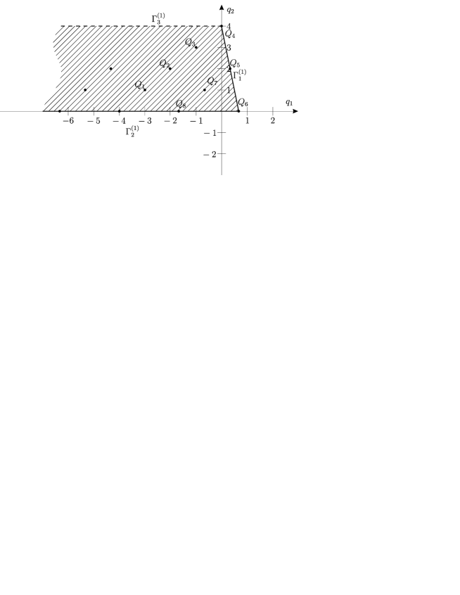
Figure 3:

The periphery of the strip contains edges $\Gamma^{(1)}_{j}\,\,(j=1,2,3)$ with normal vectors $N_{1}=(6,1),\,\,N_{2}=(0,-1),\,\,N_{3}=(0,1)$. It should take up edge $\Gamma^{(1)}_{1}$ only . This edge is corresponded by the reduced equation

$$h_{1}^{(1)}(z,\zeta)\stackrel{{\scriptstyle def}}{{=}}\zeta^{4}+18\varphi^{(l)}\zeta^{2}+72{\varphi^{(l)}}^{2}=0$$ (7.8)

Wherefrom we have

$$\zeta^{2}=-3\left(3+(-1)^{m}\right)\varphi^{(l)},\,\,\,m=1,2$$ (7.9)

We obtain twelve solutions of equation (7.8)

$$\begin{gathered}\zeta^{(l,m,k)}=g_{1/6}^{(l,m,k)}z^{1/6},\,\,\,l=1,2,3;\,\,m,k=1,2\end{gathered}$$ (7.10)

where

$$\begin{gathered}g_{1/6}^{(l,m,k)}=(-1)^{k}\sqrt{-3\left(3+(-1)^{m}\right)\,c_{1/3}^{(l)}}\,,\\ \,\,\,l=1,2,3;\,\,\,m,k=1,2\end{gathered}$$ (7.11)

The reduced equation is algebraic one, so it has no critical numbers. Let us compute the carrier of the expansion for solution of equation (7.6). The shifted carrier of equation (7.6) is contained in a lattice, generated by vectors $B_{1}=\left(\frac{7}{3},0\right),\,\,B_{2}=(1,1)$. The shifted carrier of solutions (7.10) gives rise to vector $B_{3}=\left(-\frac{1}{6},1\right)$. The difference $B_{2}-B_{3}=\left(\frac{7}{6},0\right)=\frac{1}{2}B_{1}\stackrel{{\scriptstyle def}}{{=}}B_{4}$. Therefor, vectors $B_{1},B_{2}$ and $B_{3}$ generate the same lattice as vectors $B_{2},B_{4}$. Points of this lattice can be written as

$$Q=(q_{1},q_{2})=k(1,1)+m\left(\frac{7}{6},0\right)=\left(k+\frac{7m}{6},k\right)$$

At the line $q_{2}=-1$ we have $k=-1$, and so $q_{1}=-1+\frac{7m}{6}$. As long as the cone of the problem here is $\mathcal{K}=\left\{k<\frac{1}{6}\right\}$, then the set of the carriers of expansions $\mathbf{K}$ is

$$\mathbf{K}=\left\{\frac{1-7n}{6},n\in\mathbb{N}\right\}$$ (7.12)

The expansion for solution of equation (7.6) takes the form

$$\begin{gathered}\zeta^{(l,m,k)}=g^{(l,m,k)}_{1/6}z^{1/6}+\sum_{n}g^{(l,m,k)}_{(1-7n)/6}\,z^{(1-7n)/6},\,\,\,\\ l=1,2,3;\,\,\quad\,m=1,2;\,\,\quad\,k=1,2\end{gathered}$$ (7.13)

Coefficients $g_{1/6}^{(l,m,k)}$ are determined by expression (7.11). Coefficient $g^{(l,m,k)}_{-1}$ takes on a value

$$g_{-1}^{(l,m,k)}=-\frac{1}{4}\\$$ (7.14)

The expansion of solution with taking into account four terms takes the form

$$\begin{gathered}\zeta^{(l,m,k)}=g_{{1/6}}\,{z}^{1/6}-\frac{1}{4}\,{z}^{-1}-{\frac{7}{288}}\,\frac{\left(17\,{g_{{1/6}}}^{2}+63\,c_{{1/3}}\right)}{g_{{1/6}}\left({g_{{1/6}}}^{2}+9\,c_{{1/3}}\right)}\,{z}^{-13/6}-\\ -{\frac{49}{1728}}\,{\frac{17\,{g_{{1/6}}}^{4}+36\,c_{{1/3}}{g_{{1/6}}}^{2}+567\,{c_{{1/3}}}^{2}}{{g_{{1/6}}}^{2}\left({g_{{1/6}}}^{2}+9\,c_{{1/3}}\right)^{2}}\,{z}^{-10/3}}+\ldots\end{gathered}$$ (7.15)

In view of (7.5) we can find additions $u^{(l,m,k)}(z)$. We have

$$u^{(l,m,k)}(z)=C\exp\int\zeta^{(l,m,k)}(z)dz$$

Wherefrom we get

$$\begin{gathered}u^{(l,m,k)}(z)=C_{1}\,z^{-1/4}\,\exp\left[\frac{6}{7}\,g^{(l,m,k)}_{1/6}\,z^{7/6}+\sum^{\infty}_{n=2}\frac{6}{7(1-n)}g^{(l,m,k)}_{(1-7n)/6}z^{7(1-n)/6}\right]\\ \,\,l=1,2,3;\,\quad\,m=1,2;\,\quad\,k=1,2\end{gathered}$$ (7.16)

Here $C_{1}$ and farther $C_{2}$ and $C_{3}$ are the arbitrary constants. Addition $u^{(l,m,k)}(z)$ near $z\rightarrow\infty$ is the exponentially small one in those sectors of complex plane $z$, where

$$Re\left[g^{(l,m,k)}_{7/6}\,z^{1/6}\right]<0$$ (7.17)

Thus for three expansions $G^{(1)}_{3}l$ we get four one-parameter family of additions $G_{3}^{(1)}lG^{1}_{1}mk$, where $m=1,2$ and $k=1,2$.

8 ​​​​​​.   Exponential additions of the second level.

Let us find exponential additions of the second level $v^{(p)}$, i.e. the additions to solutions $u^{(l,m,k)}(z)$. The reduced equation for addition $v^{(p)}$ is

$$M_{p}^{(2)}(z)v^{(p)}=0$$ (8.1)

where operator $M_{p}^{(2)}$ is the first variation of (7.6). Equation (8.1) for $v=v^{(p)}$ takes the form

$$\begin{gathered}\frac{d^{3}v}{dz^{3}}+4\zeta_{zz}v+4\zeta v_{zz}+6\zeta_{z}v_{z}+12\zeta\zeta_{z}v+\\ +6\zeta^{2}v_{z}+4\zeta^{3}v+18\varphi^{(l)}v_{z}+36\varphi^{(l)}\zeta v+18\varphi_{z}^{(l)}v=0\end{gathered}$$ (8.2)

Assumed that

$$\frac{d\ln v}{dz}=\xi$$ (8.3)

we have

$$\frac{dv}{dz}=\xi v,\,\,\quad\,\frac{d^{2}v}{dz^{2}}=\xi_{z}v+\xi^{2}v,\,\,\quad\,\frac{d^{3}v}{dz^{3}}=\xi_{zz}v+3\xi\xi_{z}v+\zeta^{3}v$$ (8.4)

From (8.2) we get equation

$$\begin{gathered}\xi_{zz}+3\,\xi\,\xi_{z}+\xi^{3}+4\zeta_{zz}+4\xi_{z}\,\zeta+4\xi^{2}\,\zeta+6\,\xi\,\zeta_{z}+12\zeta\zeta_{z}+6\,\xi\,\zeta^{2}+\\ +4\,\zeta^{3}+18\,\varphi^{(l)}\xi+36\,\zeta\,\varphi^{(l)}+18\,\varphi_{z}^{(l)}=0\end{gathered}$$ (8.5)

Monomials of equation (8.5) are corresponded by the points

$$\begin{gathered}M_{0,k}=\left(\frac{1}{2}-\frac{7}{6}k,\,0\right),\quad M_{1,k}=\left(\frac{1}{3}-\frac{7}{6}k,1\right),\\ M_{2,k}=\left(\frac{1}{6}-\frac{7}{6}k,\,2\right),\quad M_{3}=(0,3)\\ k=0,1,2,\ldots\end{gathered}$$ (8.6)

The carrier of the equation (8.5) is determined by points of the set (8.6). The convex set forms the strip, which is represented at fig. 4. It should examine edge $\Gamma_{1}^{(1)}$, which is passing through points

$$\begin{gathered}Q_{0}=\left(\frac{1}{2},0\right),\quad Q_{1}=\left(\frac{1}{3},1\right),\quad Q_{2}=\left(\frac{1}{6},2\right),\quad Q_{3}=\left(0,3\right)\end{gathered}$$ (8.7)

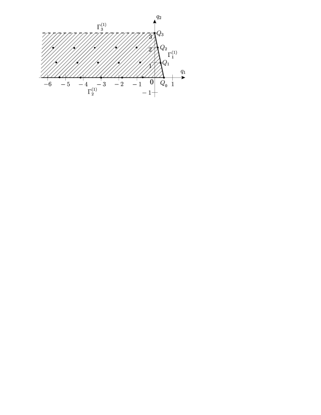
Figure 4:

The reduced equation, corresponding to this edge, is

$$\begin{gathered}\xi^{3}+4\,\xi^{2}\,\zeta+6\,\xi\,\zeta^{2}+4\,\zeta^{3}+18\,\xi\,\varphi^{(l)}+36\,\zeta\,\varphi^{(l)}=0\end{gathered}$$ (8.8)

The basis of the lattice, corresponding to the carrier of equation (8.5) is

$$\begin{gathered}B_{1}=(1,1),\,\,\,\,B_{2}=\left(\frac{7}{6},0\right)\end{gathered}$$

The solution of equation (8.8) takes the form

$$\begin{gathered}\xi^{(l,m,k,p)}=r_{1/6}^{(l,m,k,p)}\,z^{1/6},\,\,\,\,m,k=1,2;\,\,\,\,l=1,2,3;\,\,\,\,p=1,2,3\end{gathered}$$ (8.9)

where $r=r_{1/6}^{(l,m,k,p)},\,\,\,p=1,2,3$ are the roots of the equation

$$\begin{gathered}r^{3}+4\,r^{2}\,g_{1/6}^{(l,m,k)}+\left(6\,{g_{1/6}^{(l,m,k)}}^{2}+18\,c_{1/3}^{(l)}\right)\,r+4\,{g_{1/6}^{(l,m,k)}}^{3}+\\ +36\,g_{1/6}^{(l,m,k)}\,c_{1/3}^{(l)}=0\end{gathered}$$ (8.10)

Equation (8.10) has the roots

$$\begin{gathered}r_{1/6}^{(l,m,k,1)}=-2\,g_{1/6}^{(l,m,k)},\,\quad\,r_{1/6}^{(l,m,k,2)}=-g_{1/6}^{(l,m,k)}+\left(-18\,c_{1/3}^{(l)}-{g_{1/6}^{(l,m,k)}}^{2}\right)^{1/2}\\ r_{1/6}^{(l,m,k,3)}=-g_{1/6}^{(l,m,k)}-\left(-18\,c_{1/3}^{(l)}-{g_{1/6}^{(l,m,k)}}^{2}\right)^{1/2}\end{gathered}$$ (8.11)

The set of carriers of expansions for solution $\mathbf{K}$ coincides with (7.12). The expansion of solution for $\xi^{(l,m,k,p)}$ takes the form

$$\begin{gathered}\xi^{(l,m,k,p)}=r_{1/6}^{(l,m,k,p)}z^{1/6}+\sum_{n=1}^{\infty}r^{(l,m,k,p)}_{(1-7n)/6}\,z^{(1-7n)/6},\\ \,\quad\,l=1,2,3;\,\,\quad\,m=1,2;\,\,\quad\,k=1,2;\,\quad\,p=1,2,3\end{gathered}$$ (8.12)

The computing the coefficient $r_{-1}^{(l,m,k,p)}$ gives a result $r_{-1}^{(l,m,k,p)}=1/6$. The expansion of solution with taking into account three terms is

$$\begin{gathered}\xi^{(l,m,k,p)}=r_{{1/6}}{z^{1/6}}+\frac{1}{6}\,{z}^{-1}+\frac{7}{72}\,\left(34\,{g_{{1/6}}}^{3}r_{{1/6}}+{}\right.\\ \left.{}+36\,c_{{1/3}}r_{{1/6}}g_{{1/6}}+36\,c_{{1/3}}{g_{{1/6}}}^{2}+63\,c_{{1/3}}{r_{{1/6}}}^{2}+17\,{g_{{1/6}}}^{2}{r_{{1/6}}}^{2}+{}\right.\\ \left.{}+567\,{c_{{1/3}}}^{2}+17\,{g_{{1/6}}}^{4}\right)\left(g_{1/6}\right)^{-1}\left({g_{{1/6}}}^{2}+9\,c_{{1/3}}\right)^{-1}\\ \left(8\,g_{{1/6}}r_{{1/6}}+3\,{r_{{1/6}}}^{2}+6\,{g_{{1/6}}}^{2}+18\,c_{{1/3}}\right)^{-1}\,{z}^{-13/6}+\ldots\end{gathered}$$ (8.13)

The exponential additions $v^{(l,m,k,p)}(z)$ to solutions $u^{(l,m,k)}(z)$ are

$$\begin{gathered}v^{(l,m,k,p)}(z)=C_{2}\,z^{1/6}\exp\left[\frac{6}{7}\,r^{(l,m,k,p)}_{1/6}\,z^{7/6}+\sum^{\infty}_{n=2}\frac{6}{7(1-n)}r^{(l,m,k,p)}_{(1-7n)/6}z^{7(1-n)/6}\right],\\ l=1,2,3;\,\quad\,m=1,2;\,\quad\,k=1,2;\,\quad\,p=1,2,3\end{gathered}$$ (8.14)

9 ​​​​​​.   Exponential additions of the third level.

Let us compute the exponential additions of the third level $y^{(s)}$, i.e. the additions to the solutions $v^{(l,m,k,p)}(z)$. The reduced equation for addition $y^{(s)}$ is

$$M_{s}^{(3)}(z)y^{(s)}=0$$ (9.1)

Operator $M_{s}^{(3)}$ is the first variation of (8.5). Equation (9.1) for $y=y^{(l,m,k,p,s)}$ takes the form

$$\begin{gathered}y_{zz}+3\xi_{z}y+3\xi y_{z}+3\xi^{2}\,y+4\,\zeta\,y_{z}+8\,\xi\,\zeta\,y+\\ +6\zeta_{z}\,y+6\zeta^{2}\,y+18\,\varphi^{(l)}\,y=0\end{gathered}$$ (9.2)

Using the substitute

$$\frac{d\ln y}{dz}=\eta$$ (9.3)

we obtain

$$\frac{dy}{dz}=\eta y,\,\,\quad\,\frac{d^{2}y}{dz^{2}}=\eta_{z}y+\eta^{2}y$$ (9.4)

From (9.4) we have equation

$$\begin{gathered}\eta_{z}+\eta^{2}+3\xi_{z}+3\xi\eta+3\xi^{2}+4\,\eta\,\zeta+8\,\xi\,\zeta+6\zeta_{z}+6\zeta^{2}+18\,\varphi^{(l)}=0\end{gathered}$$ (9.5)

Monomials of equation (9.5) are corresponded by points

$$\begin{gathered}M_{0,k}=\left(\frac{1}{3}-\frac{7}{6}k,\,0\right),\quad M_{1,k}=\left(\frac{1}{6}-\frac{7}{6}k,\,1\right),\quad M_{2}=\left(0,\,2\right),\\ k=0,1,2\ldots\end{gathered}$$ (9.6)

The carrier of equation (9.5) is formed by points (9.6). The convex set forms the strip, which is represented at fig. 5. It should examine edge $\Gamma_{1}^{(1)}$, which is passing through points

$$\begin{gathered}Q_{0}=\left(\frac{1}{3},0\right),\,\,\,Q_{1}=\left(\frac{1}{6},1\right),\,\,\,Q_{2}=\left(0,2\right)\end{gathered}$$ (9.7)

Figure 5:

The reduced equation, corresponding to this edge, is

$$\begin{gathered}\eta^{2}+3\xi\eta+3\xi^{2}+4\,\eta\,\zeta+8\,\xi\,\zeta+6\,\zeta^{2}+18\,\varphi^{(l)}=0\end{gathered}$$ (9.8)

The solutions of equation (9.8) takes the form

$$\begin{gathered}\eta^{(l,m,k,p,s)}=q^{(l,m,k,p,s)}\,z^{1/6}\\ l=1,2,3;\,\,\,\,m,k=1,2;\,\,\,\,p=1,2,3;\,\,\,\,s=1,2;\end{gathered}$$ (9.9)

where $q^{(l,m,k,p,s)}=q$ are the roots of equation

$$\begin{gathered}q^{2}+\left(3\,r_{1/6}^{(l,m,k,p)}+4\,g_{1/6}^{(l,m,k)}\right)q+8\,r_{1/6}^{(l,m,k,p)}\,g_{1/6}^{(l,m,k)}+\\ +6\,{g_{1/6}^{(l,m,k)}}^{2}+3\,{r_{1/6}^{(l,m,k,p)}}^{2}+18\,c_{1/3}^{(l)}=0\end{gathered}$$ (9.10)

The roots of equation (9.10) are

$$\begin{gathered}q_{1/6}^{(l,m,k,p,s)}=-\frac{3}{2}\,r_{1/6}^{(l,m,k,p)}-2\,g_{1/6}^{(l,m,k)}+\\ +(-1)^{s-1}\,\left({-\frac{3}{4}\,{r_{1/6}^{(l,m,k,p)}}^{2}-2\,{r_{1/6}^{(l,m,k,p)}}\,g_{1/6}^{(l,m,k)}-2\,{g_{1/6}^{(l,m,k)}}^{2}-18\,c_{1/3}^{(l)}}\right)^{1/2},\\ l=1,2,3;\,\,\,\,m,k=1,2;\,\,\,\,p=1,2,3;\,\,\,\,s=1,2;\end{gathered}$$ (9.11)

The basis of the lattice, corresponding to the carrier of equation (9.7), is

$$\begin{gathered}B_{1}=(1,1),\,\,\,\,B_{2}=\left(\frac{7}{6},0\right)\end{gathered}$$

The set of carriers of expansions for solution $\mathbf{K}$ coincides with (7.12). The expansion of solution for $\eta^{(l,m,k,p,s)}$ takes the form

$$\begin{gathered}\eta^{(l,m,k,p,s)}=q^{(l,m,k,p,s)}_{1/6}z^{1/6}+\sum_{n=1}^{\infty}q^{(l,m,k,p,s)}_{(1-7n)/6}\,z^{(1-7n)/6},\,\,\,\\ l=1,2,3;\,\,\quad\,m=1,2;\,\,\quad\,k=1,2;\,\,\quad\,p=1,2,3;;\,\,\quad\,s=1,2;\end{gathered}$$ (9.12)

Coefficients $q^{(l,m,k,p,s)}_{1/6},\,\,s=1,2$ are determined by formulas (9.11). The computing of the coefficient $q^{(l,m,k,p,s)}_{-1}$ gives a result $q^{(l,m,k,p,s)}_{-1}=1/6$. Exponential additions $y^{(s,p,l,m,k)}(z)$ to the solutions $v^{(l,m,k,p)}(z)$ are

$$\begin{gathered}y^{(l,m,k,p,s)}(z)=C_{3}\,z^{1/6}\\ \exp\left[\frac{6}{7}\,q^{(l,m,k,p,s)}_{1/6}\,z^{7/6}+\sum^{\infty}_{n=2}\frac{6}{7(1-n)}q^{(l,m,k,p,s)}_{(1-7n)/6}z^{7(1-n)/6}\right]\\ l=1,2,3;\,\quad\,m=1,2;\,\quad\,k=1,2;\,\quad\,p=1,2,3;\,\quad\,s=1,2\end{gathered}$$ (9.13)

Thus we find three levels of the exponential additions to the expansions for solutions of equation near point $z=\infty$.

Solution $w(z)$ at $z\rightarrow\infty$ with taking into account the exponential additions has the expansion

$$\begin{gathered}w(z)=c^{(l)}_{1/3}z^{1/3}+\frac{1}{24}\,z^{-2}+\sum^{\infty}_{n=2}c^{(l)}_{(1-7n)/3}\,z^{{(1-7n)}/{3}}+\\ +C_{1}\,z^{-1/4}\,\exp\{F_{1}(z)+C_{2}\,z^{1/6}\exp\{F_{2}(z)+C_{3}\,z^{1/6}\exp\{F_{3}(z)\}\}\}\end{gathered}$$ (9.14)

where $c_{1/3}^{(l)}$ can be computed by formulas (6.2), (6.3) and (6.4); $F_{1}(z)=F_{1}^{(l,m,k)}(z)$, $F_{2}(z)=F_{2}^{(l,m,k,p)}(z)$ and $F_{3}(z)=F_{3}^{(l,m,k,p,s)}(z)$, ($l=1,2,3;\,\,\,m,k=1,2;\,\,\,p=1,2,3;\,\,\,s=1,2$) are

$$\begin{gathered}F_{1}^{(l,m,k)}(z)=\frac{6}{7}\,g^{(l,m,k)}_{1/6}\,z^{7/6}+\sum^{\infty}_{n=2}\frac{6}{7(1-n)}g^{(l,m,k)}_{(1-7n)/6}z^{7(1-n)/6}\end{gathered}$$ (9.15)

$$\begin{gathered}F_{2}^{(p,l,m,k)}(z)=\frac{6}{7}\,r^{(l,m,k,p)}_{1/6}\,z^{7/6}+\sum^{\infty}_{n=2}\frac{6}{7(1-n)}r^{(l,m,k,p)}_{(1-7n)/6}z^{7(1-n)/6}\end{gathered}$$ (9.16)

$$\begin{gathered}F_{3}^{(l,m,k,p,s)}(z)=\frac{6}{7}\,q^{(l,m,k,p,s)}_{1/6}\,z^{7/6}+\sum^{\infty}_{n=2}\frac{6}{7(1-n)}q^{(l,m,k,p,s)}_{(1-7n)/6}z^{7(1-n)/6}\end{gathered}$$ (9.17)

Coefficients $g^{(l,m,k)}_{1/6}$, $r^{(l,m,k,p)}_{1/6}$ and $q^{(l,m,k,p,s)}_{1/6}$ are defined by formulas (7.11), (8.11) and (9.11). The other coefficients are computed sequentially.

10 ​​​​​​.   Conclusion.

Let us formulate the results of this work.

All the power asymptotic forms for equation (2.1) were found.

We also found all the power expansions, corresponding to these asymptotic forms. We denote the obtained families as $G_{1}^{(0)}1$, $G_{1}^{(0)}2$, $G_{1}^{(0)}3$, $G_{1}^{(0)}4$, $G_{1}^{(1)}1$, $G_{2}^{(1)}1$ and $G_{2}^{(1)}2$ (these expansions converge for sufficiently small $|z|$). The existence and analyticity of these expansions follow from Cauchy theorem.

We found three families of expansions near $z=\infty$. That are families $G_{3}^{(1)}l\,\,(l=1,2,3)$, described by formulas (6.2), (6.3) and (6.4). For each of these expansions we found four exponential additions $G_{3}^{(1)}lG_{1}^{1}mk\,\,(m,k=1,2)$ expressed by formula (7.16). For them it was computed exponential additions $G_{3}^{(1)}lG_{1}^{1}mkG_{1}^{(1)}p\,\,(m,k=1,2;p=1,2,3)$, and then for them the proper exponential additions $G_{3}^{(1)}lG_{1}^{(1)}mkG_{1}^{(1)}pG_{1}^{(1)}s\,\,(m,k=1,2;p=1,2,3;s=1,2)$ were found too.

Families $G_{2}^{(1)}l\,\,$ and $G_{2}^{(1)}2$ were first found in the paper [3, 14, 16, 9]. However the structure of expansions $G_{2}^{(1)}1$ and $G_{2}^{(2)}2$ was not discussed earlier. The other families of expansions of solution are found for the first time.

Comparing the power expansions of equation (2.1) with power expansions of Painlevé equations $P_{1}\div P_{6}$ [21, 19, 22, 23] we note, that they differ. This fact can be interpreted as the additional prove for the hypothesis, that the fourth-order equation (2.1) determines new transcendental functions just as equations $P_{1}\div P_{6}$.

References

1.Kudryashov N.A. The first and second Painlevé equations of higher order and
some relations between them // Phys. Letters. A. 1997. V. 224. N 6.
P. 353–360.
2.Kudryashov N.A. The analitical theory of nonlinear differential equations.
Moscow – Izhevsk: The institute of compute investigations, 2004.
360 p. (in Russian)
3.Kudryashov N.A. Two hierarchies of ordinary differential equations and
their properties.// Phys. Letters. A. 1999. V. 252. P. 173–179.
4.Kudryashov N.A. Fourth-order analogies to the Painlevé equations // J. Phys.
A.: Math. Gen. 2002. V. 35. N 21. P. 4617–4632.
5.Kudryashov N.A. Amalgamations of the Painlevé equations // J. Math.
Phys., 2003, V. 44. N 12. P. 6160–6178
6.Clarkson P.A., Hone A.N.W., Joschi N. Hierarchies of difference equations
and Backlund transformations, Journal of Nonlinear Mathematical
physics, v. 10, 2003
7.Cosgrove C.M. Higher - order Painleve equations in the polynomial class. I. Bureau
symbol P2, Study Appl. Math., v. 104, 2000, 1- 65
8.Creswell G., Joshi N. The discrete first,second and thirty - fourth Painleve hierarchies,
Journal of Physics A, Math. Gen., v. 32, 1999, 655–669
9. Gordoa P.R., Pickering A. Nonisospectral scattering problems: a key to integrable hierarhies,
Journal of Mathematical Physics, v. 40, N 11, 1999, 5749–5786
10.Hone Andrew N.W. Non –autonomous Hénon — Heiles system // Physica D. 1998. V. 118 P. 1 – 16.
11.Kawai T., Koike T., Nishikawa Y., Takei Y. On the complete description of the
Stokes geometry for the first painleve hierarchy, 2004,
preprint/RS/RIMS 1471, Kioto
12.Mugan U., Jrad F. Painleve test and the first Painleve hierarchy,
Journal of Physics A, Math. Gen., v. 32, 1999, 7933–7952
13.Mugan U., Jrad F. Painleve test and higher order differential equations,
Journal of Nonlinear Mathematical Physics, v. 9, N 3, 2002, 282–310
14.Kudryashov N.A. Double Bäcklund transformations
and special integrals for the hierarhy.// Phys. Letters.
A. 2000. V. 273. P. 194–202.
15.Kudryashov N.A. Transcendents defined by nonlinear
fourth-order ordinary differential equations // J. Phys. A.: Math.
Gen. 1999. V. 32. N 6. P. 999–1013.
16.Kudryashov N.A. Nonlinear differential fourth-order equations
with transcendental solutions, Theoretical and mathematical physics,
v. 122, N 1, 2000, P. 72 - 86. (in Russian)
17.Bruno A.D. Power geometry in the algebraic and differential equations,
M., Nauka, Phismatlit, 1998, 288 p. (in Russian)
18.Bruno A.D.
Asymptotics and Expansions of Solutions to an Ordinary Differential
Equation, v.59, YMN, v. 3, 2004, p. 31-80. (in Russian)
19.Bruno A.D., Petrovich V.Y. Singularities of solutions to the first Painlevé equation,
KIAM Preprint N 9, Moscow. (in Russian)
20.Bruno A.D., Kudryashov N.A.
Asymptotic forms and power expansions for solution of the analog to
the first Painlevé equation. //Keldysh Institut of Applied
Mathematics, Preprint N 17, 2005, 26 pp.
21.Golubev V.V. The lectures on integration of motion the heavy
solid body about the fixed point. M.: Gostexizdat, 1953. 288 c. (in
Russian)
22.Bruno A.D. Power Geometry as a new calculus, in book H.G.W. Begehr
et al (eds) Analysis and Applications, ISAAC, 2001, 51-71, 2003 Kluwer
23.Gromak V.I., Laine I., Shimomura S. Painleve Differential Equations in
the Complex Plane, Walter de Gruyter, Berlin, New York, 2002.