Feshbach Resonance Management of Bose-Einstein Condensates in Optical Lattices

Abstract

We analyze gap solitons in trapped Bose-Einstein condensates (BECs) in optical lattice potentials under Feshbach resonance management. Starting with an averaged Gross-Pitaevsky (GP) equation with a periodic potential, we employ an envelope wave approximation to derive coupled-mode equations describing the slow BEC dynamics in the first spectral gap of the optical lattice. We construct exact analytical formulas describing gap soliton solutions and examine their spectral stability using the Chebyshev interpolation method. We show that these gap solitons are unstable far from the threshold of local bifurcation and that the instability results in the distortion of their shape. We also predict the threshold of the power of gap solitons near the local bifurcation limit.

I Introduction

At sufficiently low temperatures, particles in a dilute boson gas can condense in the ground state, forming a Bose-Einstein condensate (BEC) Dalfovo et al. (1999). Under the typical confining conditions of experimental settings, BECs are inhomogeneous and the number of condensed atoms ($N$) ranges from several thousand (or less) to several million (or more). The magnetic traps that confine them are usually approximated by harmonic potentials. There are two characteristic length scales: the harmonic oscillator length $a_{ho}=\sqrt{\hbar/(m\omega_{ho})}$ [which is on the order of a few microns], where $\omega_{ho}=(\omega_{x}\omega_{y}\omega_{z})^{1/3}$ is the geometric mean of the trapping frequencies, and the mean healing length $\chi=1/\sqrt{8\pi|a|\bar{n}}$ [which is on the order of a micron], where $\bar{n}$ is the mean particle density and $a$, the (two-body) $s$-wave scattering length, is determined by the atomic species of the condensate. Interactions between atoms are repulsive when $a>0$ and attractive when $a<0$. For a dilute ideal gas, $a\approx 0$.

If considering only two-body, mean-field interactions, a dilute Bose-Einstein gas can be modeled using a cubic nonlinear Schrödinger equation (NLS) with an external potential; this is also known as the Gross-Pitaevsky (GP) equation. BECs are modeled in the quasi-one-dimensional (quasi-1D) regime when the transverse dimensions of the condensate are on the order of its healing length and its longitudinal dimension is much larger than its transverse ones Köhler (2002). The GP equation for the condensate wavefunction $\psi(x,t)$ takes the form

$$i\hbar\psi_{t}=-\frac{\hbar^{2}}{2m}\psi_{xx}+V(x)\psi+g|\psi|^{2}\psi\,,$$ (1)

where $|\psi|^{2}$ is the number density, $V(x)$ is the external trapping potential, $g=[4\pi\hbar^{2}a/m][1+\mathcal{O}(\zeta^{2})]$ is proportional to the two-body scattering length, and $\zeta=\sqrt{|\psi|^{2}|a|^{3}}$ is the dilute gas parameter Dalfovo et al. (1999); Köhler (2002).

Experimentally realizable potentials $V(x)$ include harmonic traps, quartic double-well traps, optical lattices and superlattices, and superpositions of lattices or superlattices with harmonic traps. The existence of quasi-1D (“cigar-shaped”) BECs motivates the study of lower dimensional models such as Eq. (1). We focus here on the case of spatially periodic potentials without a confining trap along the dimension of the lattice, as that is of particular theoretical and experimental interest. For example, such potentials have been used to study Josephson effects Anderson and Kasevich (1998), squeezed states Orzel et al. (2001), Landau-Zener tunneling and Bloch oscillations Morsch et al. (2001), period-multiplied wavefunctions Porter and Cvitanović (2004); Machholm et al. (2004), and the transition between superfluidity and Mott insulation at both the classical Smerzi et al. (2002) and quantum Greiner et al. (2002) levels. Moreover, with each lattice site occupied by one alkali atom in its ground state, a BEC in an optical lattice shows promise as a register in a quantum computer Vollbrecht et al. (2004).

The properties of BECs—including their shape, collective excitations, statistical fluctuations, and the formation and dynamics of their solitons and vortices—are determined by the strength and sign of their two-body atomic interactions $a$. This scattering length, and hence the coefficient of the nonlinearity in the GP equation, can be adjusted in both sign and magnitude (over a large range) by minutely adjusting a magnetic field in the vicinity of a so-called “Feshbach resonance” Donley et al. (2001); Inouye et al. (1998).

A Feshbach resonance is an enhancement in the scattering amplitude of a particle incident on a target when the energy of the former is approximately that needed to create a quasibound state of the two-particle system. If a pair of ultracold atoms has a molecular bound state near zero energy, then during collisions they stick together for a little while as they undergo a Feshbach resonance. While few molecules have bound states at such energies, one can adjust the relative energies of atoms and molecules with different magnetic moments by applying a magnetic field. With such “Zeeman tuning”, one can move the atomic energy from just above the resonance to just below it, so that the scattering length diverges and changes sign from positive to negative across the resonance.

As a result of the control this procedure gives over condensate properties, the manipulation of ultracold atoms using Feshbach resonances has become among the most active research areas in experimental atomic physics. Feshbach resonances have provided a key for creating molecular BECs, generating solitons and atom-molecule coherence, stabilizing or destabilizing BECs, and creating novel Fermi liquids Duine and Stoof (2004); Kleppner (2004); Donley et al. (2002); Regal et al. (2003). For example, it was recently shown that near a Feshbach resonance, a quantum phase transition occurs between a regime with both atomic and molecular condensates and one with only molecular condensates Romans et al. (2004). As pointed out in Ref. Dickerscheid et al. (2005), this transition should be much easier to observe for condensates loaded into optical lattice potentials.

In Feshbach resonance management, which was motivated by similar techniques in fiber optics Kurtzke (1993), the BEC scattering length is varied periodically in time. This yields dynamically interesting soliton solutions, such as breathers Kevrekidis et al. (2003b). Very recently, there has been some theoretical work concerning Feshbach resonances in BECs in optical lattices Abdullaev et al. (2003); Brazhnyi and Konotop (2005); Matuszewski et al. (To appear). This situation is also the subject of current experimental investigations Köhl et al. (2005).

In the present paper, we use an averaged GP equation Pelinovsky et al. (2004a); Zharnitsky and Pelinovsky (2005) to examine gap solitons in BECs trapped in optical lattices and under the influence of Feshbach resonance management. Using an envelope-wave approximation, we derive coupled-mode equations describing the slow dynamics of gap solitons. We provide an analytical construction of gap soliton solutions and examine their spectral stability with numerical computations of eigenvalues. We then describe the time-evolution of gap solitons with the averaged and original GP equations. Finally, we summarize our results.

II The averaged Gross-Pitaevsky equation

We consider the non-dimensional GP equation for trapped BECs under Feshbach resonance management,

$$i\psi_{t}=-\psi_{xx}+V(x)\psi+g(t)|\psi|^{2}\psi\,,$$ (2)

where the normalized independent variables are

$$\tilde{x}=\frac{\sqrt{2m}x}{\hbar}\,,\qquad\tilde{t}=\frac{t}{\hbar}\,,$$

and the tildes have been dropped from Eq. (2). The nonlinear coefficient can be written Kevrekidis et al. (2003b)

$$g(t)=\gamma_{0}+\frac{1}{\varepsilon}\gamma\left(\frac{t}{\varepsilon}\right)\,,$$ (3)

and the potential for optical lattices is Pelinovsky et al. (2004b)

$$V(x)=2\epsilon V_{0}\cos(\omega x)\,.$$ (4)

Here, $\gamma_{0}$ is the mean value of the nonlinearity coefficient; $\gamma(\tau)$, with $\tau=t/\varepsilon$, is a mean-zero periodic function with unit period; $\varepsilon\ll 1$ is a small parameter describing the strength of the Feshbach resonance management; $\omega$ is the wavenumber of the optical lattice; and $\epsilon V_{0}$ is a small parameter describing the strength (amplitude) of the lattice. Because (3) changes rapidly in time (i.e., the management is strong), it is reasonable use a model without dissipation Köhl et al. (2005). We note that the two small parameters $\epsilon$ and $\varepsilon$ in Eq. (2) are due to two different physical sources and can be uncorrelated.

One can exert very precise control over optical lattice strengths and wavenumbers experimentally Denschlag et al. (2004b). In particular, both strong and weak lattices can be implemented; we will consider a weak optical lattice, so that $\epsilon$ in (4) is small. In experiments, the scattering length $a$ can also be adjusted either nonadiabatically (strong nonlinearity management), which is the situation discussed in the present work, or adiabatically (weak nonlinearity management). In general, different dynamics can occur depending on how rapidly $a$ is adjusted, as discussed, e.g., in Cubizolles et al. (2003). There have already been some experiments in which Feshbach resonances are applied to BECs in the presence of optical lattices Köhl et al. (2005) and others are being planned by multiple experimental groups. As mentioned above, a conservative model is appropriate for strong nonlinearity management. For weak nonlinearity management, however, the GP equation (2) needs to be augmented by dissipation terms, as three-body recombination leads to experimental losses Donley et al. (2001); Köhl et al. (2005). Therefore, we will only consider strong management, so that $\varepsilon$ in (3) is small.

The small parameter $\varepsilon$ can be used to simplify the time-periodic GP equation (2) with an averaging method. Using the time-averaging procedure from Pelinovsky et al. (2004a), one can look for an asymptotic solution to the GP equation (2) of the form

$$\psi(x,t)=e^{i\varepsilon\gamma_{-1}(\tau)|u|^{2}(x,t)}\;\left[u(x,t)+{\rm O}(\varepsilon)\right]\,,$$ (5)

where $u$ is the complex-valued amplitude and $\gamma_{-1}(\tau)$ is the mean-zero anti-derivative of $\gamma(\tau)$. Within a regular averaging procedure (see the review in Zharnitsky and Pelinovsky (2005)), we obtain the averaged GP equation,

$$iu_{t} =-u_{xx}+2\epsilon V_{0}\cos(\omega x)u+\gamma_{0}|u|^{2}u$$

$$\quad-\gamma_{1}^{2}\left[((|u|^{2})_{x})^{2}+2|u|^{2}(|u|^{2})_{xx}\right]u\,,$$ (6)

where $\gamma_{1}$ is the standard deviation of the nonlinearity coefficient. The model (6) provides a starting point for our analysis of gap solitons in BECs in optical lattices under Feshbach resonance management. Without such management ($\gamma_{1}=0$), gap solitons of the GP equation (6) were studied in Pelinovsky et al. (2004b) using Floquet theory, multiple-scale expansions, beyond-all-orders theory, and Evans-function computations of eigenvalues. We will mainly consider the opposite case when $\gamma_{1}\neq 0$ but $\gamma_{0}=0$.

III Coupled-mode Equations

We are interested in modeling gap solitons supported by subharmonic resonances between the periodic potential and spatio-temporal solutions of the averaged GP equation (6). To simplify the model, we use the second small parameter $\epsilon$ and obtain coupled-mode equations, which averages the spatially periodic nonlinear equation (6) near a spectral gap of its associated linearization,

$$iu_{t}=-u_{xx}+2\epsilon V_{0}\cos(\omega x)u\,.$$ (7)

In the limit of small $\epsilon$, the spectral gaps all become narrow and the first spectral gap occurs at first order in $\epsilon$. Using the space-averaging technique of Ref. Agueev and Pelinovsky (1994), one can look for an asymptotic solution of the averaged GP equation (6) in the two-wave form

$$u(x,t) =\sqrt{\epsilon}\left(A(X,T)e^{i\omega_{0}x-i\omega_{0}^{2}t}\right.$$

$$\quad\left.+B(X,T)e^{-i\omega_{0}x-i\omega_{0}^{2}t}+{\rm O}(\epsilon)\right)\,,$$ (8)

where $A$ and $B$ are complex-valued amplitudes, $X=\epsilon x$ and $T=\epsilon t$ are slow variables, and $\omega=2\omega_{0}$. This wavenumber ratio indicates that we are studying $2\!:\!1$ subharmonic resonances [e.g. the first spectral gap of equation (7)]. Using the regular asymptotic procedure from Agueev and Pelinovsky (1994), we obtain a system of coupled-mode equations

$$i(A_{T}+\omega A_{X}) =V_{0}B+\gamma_{0}(|A|^{2}+2|B|^{2})A$$

$$\quad+2\gamma_{1}^{2}\omega^{2}(2|A|^{2}+|B|^{2})|B|^{2}A\,,$$

$$i(B_{T}-\omega B_{X}) =V_{0}A+\gamma_{0}(2|A|^{2}+|B|^{2})B$$

$$\quad+2\gamma_{1}^{2}\omega^{2}(|A|^{2}+2|B|^{2})|A|^{2}B\,.$$ (9)

The first equation governs the left-propagating wave $A$, whereas the second equation governs the right-propagating wave $B$. The two waves interact with a cubic cross-phase modulation from the mean value of the scattering length and with a quintic cross-phase modulation from the standard deviation of the scattering length. The latter effect represents the main contribution of Feshbach resonance management in trapped BECs.

The system of coupled-mode equations (9) is Hamiltonian, with symmetric potential energy

$$W(A,B) =V_{0}\left(\bar{A}B+A\bar{B}\right)$$

$$\quad+\frac{\gamma_{0}}{2}\left(|A|^{4}+4|A|^{2}|B|^{2}+|B|^{4}\right)$$

$$\quad+2\gamma_{1}^{2}\omega^{2}|A|^{2}|B|^{2}(|A|^{2}+|B|^{2})\,.$$ (10)

Additionally, Eq. (10) satisfies the assumption on symmetric potential functions used recently for analyzing the existence and stability of gap solitons Chugunova and Pelinovsky (2006). While the previous work concerned gap solitons in coupled-mode equations with cubic nonlinearity, we will focus on the new effects that arise from the quintic nonlinear terms. These effects correspond to mean-zero Feshbach resonance management, which affects the propagation of gap solitons in optical lattices. We can see that the last term of $W$ in (10) is positive definite, similar to the second term with $\gamma_{0}>0$. Therefore, Feshbach resonance management leads to defocusing effects on the propagation of gap solitons in periodic potentials. The defocusing role of Feshbach resonance management was studied recently in Kevrekidis et al. (2005) in the context of blow-up arrest in multi-dimensional GP equations.

One determines the linear spectrum of the coupled-mode equations (9) from the linearized system in Fourier form, $(A,B)\sim e^{iKX-i\Omega T}$, where $\Omega=\pm\sqrt{V_{0}^{2}+\omega^{2}K^{2}}$. The spectral gap exists for $|\Omega|<|V_{0}|$ and corresponds to the first spectral gap associated with the periodic potential in Eq. (7). The lower (upper) spectral band of the coupled-mode equations (9) for $\Omega<-|V_{0}|$ (for $\Omega>|V_{0}|$) corresponds to the first (second) spectral band of the periodic potential in (7).

The coupled-mode system (9) can be reduced to a nonlinear Schrödinger (NLS) equation near the band edges of the linear spectrum. Using the asymptotic representation

$$A =\sqrt{\mu}e^{\pm i|V_{0}|T}\left[W(\xi,\zeta)\pm\frac{i\mu\omega}{2V_{0}}W_{\xi}+{\rm O}(\mu^{2})\right]\,,$$ (11)

$$B =\sqrt{\mu}e^{\pm i|V_{0}|T}\left[\mp W(\xi,\zeta)+\frac{i\mu\omega}{2V_{0}}W_{\xi}+{\rm O}(\mu^{2})\right]\,,$$ (12)

where $\xi=\mu X$, $\zeta=\mu^{2}T$, and $\mu$ is a small parameter for the distance of $\Omega$ from the band edges $\pm|V_{0}|$, one can reduce the coupled-mode equations (9) with $\gamma_{0}=0$ to the quintic NLS equation:

$$iW_{\zeta}=\pm\frac{\omega^{2}}{2V_{0}}W_{\xi\xi}+6\gamma_{1}^{2}\omega^{2}|W|^{4}W\,.$$ (13)

The quintic NLS equation (13) is focusing near the lower spectral band with $\Omega=-|V_{0}|$ and is defocusing near the upper spectral band with $\Omega=|V_{0}|$. Therefore, the gap soliton solutions bifurcate from the lower spectral band via a local (small-amplitude) bifurcation. They terminate at the upper spectral band via a nonlocal (large-amplitude) bifurcation, similar to gap solitons in the GP equation with a periodic potential Pelinovsky et al. (2004b).

The derivation of the quintic NLS equation (13) confirms the predictions of the recent paper Gubeskys et al. (2005) on the power threshold for one-dimensional gap solitons in the case $\gamma_{0}=0$ and $\gamma_{1}\neq 0$. The existence of the power threshold near the local bifurcation limit was computed numerically in Ref. Gubeskys et al. (2005). Because the quintic NLS equation exhibits a similar power threshold for NLS solitons (see, e.g., Pelinovsky et al. (1998)), the numerical fact is now confirmed from the perspective of asymptotic theory. We note that the coupled-mode equations (9) with $\gamma_{0}\neq 0$ reduce to the cubic NLS equation, which does not exhibit the power threshold for NLS solitons.

IV Gap Solitons

We simplify the construction of exact gap soliton solutions to the coupled-mode equations (9) by normalizing $V_{0}=-1$, $\omega=1$ (a standard scaling transformation can be employed for this purpose) and defining $\sigma^{2}=2\gamma_{1}^{2}\omega^{2}$. We construct gap soliton solutions by separating variables into time-periodic and spatially localized solutions of the coupled-mode equations (9):

$$A(X,T)=a(X)e^{-i\Omega T}\,,\quad B(X,T)=b(X)e^{-i\Omega T}\,.$$

Because of the symmetry in the potential function, $W(A,B)=W(B,A)$, the gap soliton solutions satisfy the constraint $b=\bar{a}$ Chugunova and Pelinovsky (2006), so that $a(X)$ solves the following nonlinear ordinary differential equation:

$$ia^{\prime}+\Omega a+\bar{a}=3\gamma_{0}|a|^{2}a+3\sigma^{2}|a|^{4}a\,.$$

Converting the function $a(X)$ to polar coordinates,

$$a(X)=\sqrt{Q(X)}\exp[-i\Theta(X)/2]\,,$$ (14)

we obtain the second-order system,

$$Q^{\prime} =-2Q\sin\Theta\,,$$

$$\Theta^{\prime} =-2\Omega-2\cos\Theta+6\gamma_{0}Q+6\sigma^{2}Q^{2}\,.$$ (15)

This system has the first integral

$$E=-\Omega Q-Q\cos\Theta+\frac{3}{2}\gamma_{0}Q^{2}+\sigma^{2}Q^{3}\,,$$ (16)

where $E=0$ from the zero boundary conditions $Q(X)\to 0$ as $|X|\to\infty$.

In the remainder of this paper, we consider the case $\gamma_{0}=0$ and $\gamma_{1}\neq 0$, which shows the effects of Feshbach resonance management on the existence and stability of gap solitons. For the case $\gamma_{0}\neq 0$ and $\gamma_{1}=0$, exact analytical solutions for gap solitons are available de Sterke and Sipe (1994) and the stability problem has been analyzed numerically (see Chugunova and Pelinovsky (2006)). When $\gamma_{0}=0$, the second-order system (15) reduces to the first-order differential equation,

$$\Theta^{\prime}=4(\Omega+\cos\Theta)\,.$$ (17)

The function $Q(X)$ is found from $\Theta(X)$ with the relation

$$Q^{2}=\frac{\Omega+\cos\Theta}{\sigma^{2}}\geq 0\,.$$ (18)

Using the technique from Appendix A of Chugunova and Pelinovsky (2006), we find the exact analytical solution of Eq. (17) and obtain

$$\cos\Theta=\frac{\cosh^{2}{(2\beta x)}-\gamma\sinh^{2}{(2\beta x)}}{\cosh^{2}{(2\beta x)}+\gamma\sinh^{2}{(2\beta x)}}\,,$$ (19)

where

$$\gamma=\frac{1+\Omega}{1-\Omega}\,,\qquad\beta=\sqrt{1-\Omega^{2}}\,,$$

and $|\Omega|<1$. Substituting (19) into (18) then gives

$$Q^{2}=\frac{1}{\sigma^{2}}\frac{1+\Omega}{\cosh^{2}{(2\beta x)}+\gamma\sinh^{2}{(2\beta x)}}\,,$$ (20)

so that

$$a(X)=\frac{\sqrt[4]{\gamma(\cosh{(4\beta X)}-\Omega)}}{\sqrt{\sigma}[\cosh(2\beta X)+i\sqrt{\gamma}\sinh(2\beta X)]}$$ (21)

and

$$|a|^{2}=\frac{\beta}{\sigma\sqrt{\cosh(4\beta X)-\Omega}}\,.$$ (22)

The limit $\Omega\to-1$ yields the small-amplitude gap soliton $|a|^{2}\to({\beta}/{\sigma\sqrt{2}})\;{\rm sech}(2\beta X)$, which satisfies the focusing quintic NLS equation (13). At this local bifurcation limit, the power of the gap soliton has a threshold,

$$P\equiv\int_{-\infty}^{\infty}\left(|A|^{2}+|B|^{2}\right)dX\to P_{0}\equiv\frac{\pi}{\sigma\sqrt{2}}\,,$$

such that the power $P$ is bounded from below by the limiting value $P_{0}$. The opposite limit $\Omega\to+1$ yields the large-amplitude (singular) gap soliton $|a|^{2}\to({\beta}/{\sigma\sqrt{2}}){\rm csch}(2\beta X)$, which satisfies the corresponding defocusing quintic NLS equation (13). Thus, in accordance with the asymptotic reduction to the quintic NLS equation (13), the family of gap soliton solutions of the coupled-mode system (9) bifurcates from the lower spectral band ($\Omega=-1$) and terminates at the upper spectral band ($\Omega=+1$).

IV.1 Stability

The spectral stability of the gap soliton (21) follows from the linearization

$$\left\{\begin{array}[]{c}A(X,T)=e^{-i\Omega T}\left(a(X)+U_{1}(X)e^{\lambda T}\right)\\ \bar{A}(X,T)=e^{i\Omega T}\left(\bar{a}(X)+U_{2}(X)e^{\lambda T}\right)\\ B(X,T)=e^{-i\Omega T}\left(\bar{a}(X)+U_{3}(X)e^{\lambda T}\right)\\ \bar{B}(X,T)=e^{i\Omega T}\left(a(X)+U_{4}(X)e^{\lambda T}\right)\end{array}\right.\,.$$ (23)

The vector ${\bf U}=(U_{1},U_{2},U_{3},U_{4})^{T}$ solves the linear eigenvalue problem,

$$H_{\omega}{\bf U}=i\lambda s{\bf U}\,,$$ (24)

where $s=\mbox{diag}(1,-1,1,-1)$ is a diagonal matrix. The linearized energy operator $H_{\omega}$ has the form

$$H_{\omega}=D(\partial_{X})+\mathcal{V}(X)\,,$$ (25)

where

$$D=\left(\begin{array}[]{cccc}-\Omega-i\partial_{X}&0&-1&0\\ 0&-\Omega+i\partial_{X}&0&-1\\ -1&0&-\Omega+i\partial_{X}&0\\ 0&-1&0&-\Omega-i\partial_{X}\end{array}\right)$$

and

$$\mathcal{V}=\sigma^{2}\left(\begin{array}[]{cccc}5|a|^{4}&2|a|^{2}a^{2}&4|a|^{2}a^{2}&4|a|^{4}\\ 2|a|^{2}\bar{a}^{2}&5|a|^{4}&4|a|^{4}&4|a|^{2}\bar{a}^{2}\\ 4|a|^{2}\bar{a}^{2}&4|a|^{4}&5|a|^{4}&2|a|^{2}\bar{a}^{2}\\ 4|a|^{4}&4|a|^{2}a^{2}&2|a|^{2}a^{2}&5|a|^{4}\end{array}\right)\,.$$

Using the block-diagonalization method from Chugunova and Pelinovsky (2006), we employ the orthogonal similarity matrix

$$S=\frac{1}{\sqrt{2}}\left(\begin{array}[]{cccc}1&0&1&0\\ 0&1&0&1\\ 0&1&0&-1\\ 1&0&-1&0\end{array}\right)$$

that simultaneously block-diagonalizes the energy operator $H_{\omega}$,

$$S^{-1}H_{\omega}S=\left(\begin{array}[]{cc}H_{+}&0\\ 0&H_{-}\end{array}\right)\equiv H,$$ (26)

and the linearized operator $sH_{\omega}$,

$$S^{-1}sH_{\omega}S=s\left(\begin{array}[]{cc}0&H_{-}\\ H_{+}&0\end{array}\right)\equiv iL\,,$$ (27)

where $H_{\pm}$ are two-by-two Dirac operators:

$$H_{+} =\left(\begin{array}[]{cc}-\Omega-i\partial_{X}+9\sigma^{2}|a|^{4}&6\sigma^{2}|a|^{2}a^{2}-1\\ 6\sigma^{2}|a|^{2}\bar{a}^{2}-1&-\Omega+i\partial_{X}+9\sigma^{2}|a|^{4}\end{array}\right)\,,$$ (30)

$$H_{-} =\left(\begin{array}[]{cc}-\Omega-i\partial_{X}+\sigma^{2}|a|^{4}&1-2\sigma^{2}|a|^{2}a^{2}\\ 1-2\sigma^{2}|a|^{2}\bar{a}^{2}&-\Omega+i\partial_{X}+\sigma^{2}|a|^{4}\end{array}\right)\,.$$ (33)

Eigenvalues of the operators $L$, $H_{+}$, and $H_{-}$ are detected numerically with the Chebyshev interpolation method Chugunova and Pelinovsky (2006). The main advantage of the Chebyshev grid is that clustering of the grid points occurs near the end points of the interval. This prevents the appearance of spurious complex eigenvalues that may otherwise arise from the discretization of the continuous spectrum. Moreover, by using the block-diagonalization in (26)–(27), we are able to reduce the memory constraints and double the speed of the numerical computations (see the details in Chugunova and Pelinovsky (2006)).

The numerical eigenvalues of the operators $L$, $H_{+}$, and $H_{-}$ are displayed in Fig. 1 for six different values of the parameter $\Omega$. When $\Omega$ is close to the local bifurcation threshold (e.g., for $\Omega=-0.9$), the operator $L$ has a four-dimensional kernel at $\lambda=0$ and a pair of small purely imaginary eigenvalues near $\lambda=0$. The pair of purely imaginary eigenvalues originates from the six-dimensional kernel of the linearized quintic NLS equation (13) (see, e.g., Ref. Pelinovsky et al. (1998)). In this case, the operator $H_{+}$ has no isolated non-zero eigenvalues, whereas the operator $H_{-}$ has a simple isolated non-zero eigenvalue. The eigenvalue of $H_{-}$ still exists at $\Omega=-0.7$, but it disappears before $\Omega=-0.3$ because it collides with the end point of the continuous spectrum of $H_{-}$. The pair of eigenvalues of $L$ survives at $\Omega=-0.3$, but it disappears at $\Omega=0$ because it collides with the end points of the continuous spectrum of $L$. When $\Omega>0$, the pair of complex eigenvalues bifurcates in the spectrum of $L$ from the end points of the continuous spectrum of $L$. The complex eigenvalues of $L$ bifurcate simultaneously with a simple isolated non-zero eigenvalue of the operator $H_{-}$. The pair of complex eigenvalues of $L$ and the isolated non-zero eigenvalue of $H_{-}$ persist for larger values of $\Omega$ (e.g., for $\Omega=0.3$ and $\Omega=0.7$). The eigenvalues just discussed are labeled in the figure as ${\rm I}$ and ${\rm II}$.

In sum, the gap solitons of the coupled-mode system (9) with $\gamma_{0}=0$ are spectrally stable for $\Omega<0$ and spectrally unstable due to complex unstable eigenvalues for $\Omega>0$. This behavior is similar to the stability analysis of the coupled-mode system (9) with $\gamma_{0}\neq 0$ and $\gamma_{1}=0$ (see Chugunova and Pelinovsky (2006) and references therein).

V Numerical simulations

To confirm the accuracy of the coupled-mode theory, we corroborate the instability of gap solitons for $\Omega>0$ predicted from the analysis of the system (9) with full numerical simulations of the averaged GP equation (6). We consider the trigonometric management function $\gamma(\tau)=\cos(2\pi\tau)$ and fix the other parameters as follows: $\gamma_{0}=0$, $\gamma_{1}=1/\sqrt{2}$, $V_{0}=-1$, $\omega=1$, and $\epsilon=0.1$. We vary the parameter $\Omega$ for the gap soliton solutions, focusing on computations with $\Omega=-0.5$ and $\Omega=0.5$. According to analysis of the coupled-mode equations (9), the value $\Omega=-0.5$ corresponds to the case of stable gap solitons, and the value $\Omega=0.5$ corresponds to the case of unstable gap solitons. The initial condition for all simulations is selected to be a perturbation of the leading-order two-wave approximation (III) with the gap soliton solutions (21).

We integrated the averaged GP equation (6) using a finite-difference approximation (with 480 grid points) in space and a Runge-Kutta integration scheme (with step size $h=0.001$) in time. The perturbations of the initial gap solitons are of the same functional form as the gap solitons but with larger amplitudes.

Figure 2 shows the time-evolution of a stable gap soliton with $\Omega=-0.5$. The stationary gap soliton persists in the full dynamics of the averaged GP equation (6), in agreement with the stability analysis of the coupled-mode system (9).

Figure 3 illustrates the dynamics of an unstable gap soliton with $\Omega=0.5$. We observe an asymmetric beating between different localized waveforms. The localized wave is not destroyed in the unstable case, but rather undergoes shape distortions due to the oscillatory instability. This behavior agrees with the stability analysis in the coupled-mode system (9), as the unstable eigenvalues of gap solitons with $\Omega>0$ are complex-valued (see Fig. 1). While the perturbation used in Fig. 3 is large, note that a perturbation with the same percentage difference in the soliton amplitude does not lead to an instability in Fig. 2.

We also examined the dynamics of the solutions constructed using coupled-mode theory under full numerical simulations of the original GP equation (2). In these simulations, which were also performed using a finite-difference approximation (with 480 grid points) in space and a Runge-Kutta integration scheme (with step size $h=0.001$) in time, the external potential includes contributions from a small harmonic trap in addition to the optical lattice in (4). Hence, the potential in these simulations is given by $\hat{V}(x)=V(x)+V_{h}x^{2}$. The initial conditions and parameters are the same as for the simulations of the averaged GP equation, with the additional values $\varepsilon=0.25$ and $V_{h}=0.01$. In Fig. 4, we show the spatio-temporal evolution of the constructed gap solitons under equation (2). As expected, the solitons that we found to be stable persist longer with respect to the full GP dynamics than those determined to be unstable.

VI Conclusions

In conclusion, we studied Feshbach resonance management for gap solitons in Bose-Einstein condensates trapped in optical lattice potentials. We applied an envelope wave approximation to the averaged Gross-Pitaevsky equation with a periodic potential to yield coupled-mode equations describing the slow BEC dynamics in the first spectral gap of the optical lattice. We derived exact analytical expressions for gap solitons with zero mean scattering length. In this situation, Feshbach resonances are employed to tune a condensate between the repulsive and attractive regimes (corresponding to their usual experimental application). Applying Chebyshev interpolation to the coupled-mode equations, we showed that these gap solitons are unstable above the center of the first spectral gap (far from the local bifurcation threshold). We then showed with numerical simulations of the averaged Gross-Pitaevsky (GP) equation that unstable gap solitons exhibit beating between different localized shapes, thereby confirming the stability results predicted from the coupled-mode theory. We corroborated this further with numerical simulations of the original GP equation, which show that the stable gap solitons persist much longer than the unstable ones.

We note that gap solitons in the GP equation with a periodic potential (6) and the coupled-mode system (9) in the case of no Feshbach resonance management have been studied recently in Pelinovsky et al. (2004b) and Chugunova and Pelinovsky (2006), respectively. We can see from comparing the previous and new results that Feshbach resonance management leads to a new effect with respect to the existence of the power threshold near the local bifurcation limit Gubeskys et al. (2005). On the other hand, there are not many differences in the stability results, as Feshbach resonance management does not stabilize gap solitons far from the threshold of local bifurcations (which are known to be unstable Chugunova and Pelinovsky (2006)). We have also confirmed that Feshbach resonance management leads to defocusing effects on the propagation of gap solitons, which is relevant for blow-up arrest in multi-dimensional problems Kevrekidis et al. (2005).

VII Acknowledgements

We gratefully acknowledge Jit Kee Chin, Randy Hulet, Panos Kevrekidis, Boris Malomed, and Steve Rolston for useful discussions about this project. The code for numerical simulations of the NLS was modified from the code of Panos Kevrekidis. M.A.P. acknowledges support from the NSF VIGRE program and the Gordon and Betty Moore Foundation. M. Ch. was supported by the ShacrNet and NSERC graduate scholarships. D. P. was supported by the NSERC Discovery and PREA grants.

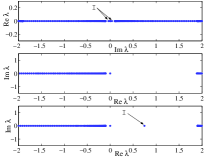
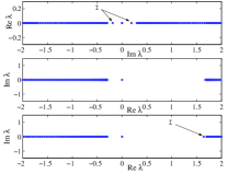
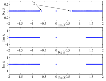
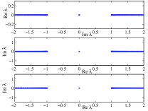
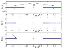
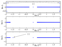
Figure 1: (Color online) Eigenvalues and instability bifurcations for the operators $L$, $H_{+}$, and $H_{-}$ in (27), (30, and (33). The parameter values are $\Omega=-0.9$ (top left), $\Omega=-0.7$ (top right), $\Omega=-0.3$ (middle left), $\Omega=0.0$ (middle right), $\Omega=0.3$ (bottom left), and $\Omega=0.7$ (bottom right).

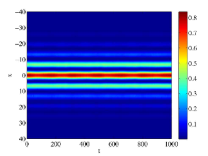
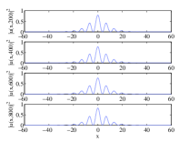
Figure 2: (Color online) Stable time-evolution of a gap soliton with $\Omega=-0.5$ in the averaged GP equation (6). (Left) Spatio-temporal evolution of $|u(x,t)|^{2}$. (Right) Spatial profiles of $|u(x,t)|^{2}$ for $t=0$, $t=200$, $t=400$, and $t=800$.

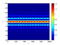
Figure 3: (Color online) Unstable time-evolution of a gap soliton with $\Omega=0.5$ in the averaged GP equation (6). (Left) Spatio-temporal evolution of $|u(x,t)|^{2}$. (Right) Spatial profiles of $|u(x,t)|^{2}$ for $t=0$, $t=200$, $t=400$, and $t=800$.

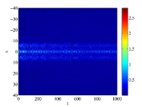
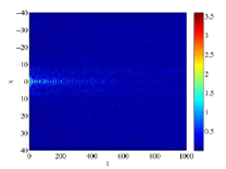
Figure 4: (Color online) Spatio-temporal evolution of $|\psi(x,t)|^{2}$, with initial conditions given by the constructed gap solitons, under the dynamics of the full GP equation (2). (Left) $\Omega=-0.5$. (Right) $\Omega=0.5$.

References

- Dalfovo et al. (1999) F. Dalfovo, S. Giorgini, L. P. Pitaevskii, and S. Stringari, Reviews of Modern Physics 71, 463 (1999).
- Köhler (2002) T. Köhler, Physical Review Letters 89, 210404 (2002).
- Anderson and Kasevich (1998) B. P. Anderson and M. A. Kasevich, Science 282, 1686 (1998).
- Orzel et al. (2001) C. Orzel, A. K. Tuchman, M. L. Fenselau, M. Yasuda, and M. A. Kasevich, Science 291, 2386 (2001).
- Morsch et al. (2001) O. Morsch, J. H. Müller, M. Cristiani, D. Ciampini, and E. Arimondo, Physical Review Letters 87, 140402 (2001).
- Machholm et al. (2004) M. Machholm, A. Nicolin, C. J. Pethick, and H. Smith, Physical Review A 69, 043604 (2004).
- Porter and Cvitanović (2004) M. A. Porter and P. Cvitanović, Physical Review E 69, 047201 (2004).
- Smerzi et al. (2002) A. Smerzi, A. Trombettoni, P. G. Kevrekidis, and A. R. Bishop, Physical Review Letters 89, 170402 (2002).
- Greiner et al. (2002) M. Greiner, O. Mandel, T. Esslinger, T. Hänsch, and I. Bloch, Nature 415, 39 (2002).
- Vollbrecht et al. (2004) K. G. H. Vollbrecht, E. Solano, and J. I. Cirac, Physical Review Letters 93, 220502 (2004).
- Donley et al. (2001) E. A. Donley, N. R. Claussen, S. L. Cornish, J. L. Roberts, E. A. Cornell, and C. E. Weiman, Nature 412, 295 (2001).
- Inouye et al. (1998) S. Inouye, M. R. Andrews, J. Stenger, H. J. Miesner, D. M. Stamper-Kurn, and W. Ketterle, Nature 392, 151 (1998).
- Donley et al. (2002) E. A. Donley, N. R. Claussen, S. T. Thompson, and C. E. Weiman, Nature 417, 529 (2002).
- Duine and Stoof (2004) R. A. Duine and H. T. C. Stoof, Physics Reports 396, 115 (2004).
- Kleppner (2004) D. Kleppner, Physics Today 57, No. 8, 12 (2004).
- Regal et al. (2003) C. A. Regal, C. Ticknor, J. L. Bohn, and D. S. Jin, Nature 424, 47 (2003).
- Romans et al. (2004) M. W. J. Romans, R. A. Duine, S. Sachdev, and H. T. C. Stoof, Physical Review Letters 93, 020405 (2004).
- Dickerscheid et al. (2005) D. B. M. Dickerscheid, A. Khawaja, D. van Osten, and H. T. C. Stoof, Physical Review A 71, 043604 (2005).
- Kurtzke (1993) C. Kurtzke, IEEE Photonics Technology Letters 5, 1250 (1993).
- Kevrekidis et al. (2003b) P. G. Kevrekidis, G. Theocharis, D. J. Frantzeskakis, and B. A. Malomed, Physical Review Letters 90, 230401 (2003b).
- Abdullaev et al. (2003) F. K. Abdullaev, E. N. Tsoy, B. A. Malomed, and R. A. Kraenkel, Physical Review A 68, 053606 (2003).
- Brazhnyi and Konotop (2005) V. A. Brazhnyi and V. V. Konotop, Physical Review A 72, 033615 (2005).
- Matuszewski et al. (To appear) M. Matuszewski, E. Infeld, B. A. Malomed, and M. Trippenbach, Physical Review Letters 95, 050403 (2005).
- Köhl et al. (2005) M. Köhl, H. Moritz, T. Stöferle, K. Günter, and T. Esslinger, Physical Review Letters 94, 080403 (2005).
- Pelinovsky et al. (2004a) D. E. Pelinovsky, P. G. Kevrekidis, D. J. Frantzeskakis, and V. Zharnitsky, Physical Review E 70, 047604 (2004a).
- Zharnitsky and Pelinovsky (2005) V. Zharnitsky and D. E. Pelinovsky, Chaos 15, 037105 (2005)
- Pelinovsky et al. (2004b) D. E. Pelinovsky, A. A. Sukhorukov, and Y. S. Kivshar, Physical Review E 70, 036618 (2004b).
- Denschlag et al. (2004b) J. Hecker Denschlag, J. E. Simsarian, H. Haffner, C. McKenzie, A. Browaeys, D. Cho, K. Helmerson, S. L. Rolston, and W. D. Phillips, Journal of Physics B: Atomic Molecular and Optical Physics 35, 3095-3110 (2002b).
- Cubizolles et al. (2003) J. Cubizolles, T. Bourdel, S. J. J. M. F. Kokkelmans, G. V. Shlyapnikov, and C. Salomon, Physical Review Letters 91, 240401 (2003).
- Agueev and Pelinovsky (1994) D. Agueev and D. Pelinovsky, SIAM Journal of Applied Mathematics 65, 1101 (2005).
- Chugunova and Pelinovsky (2006) M. Chugunova and D. E. Pelinovsky, SIAM Journal of Applied Dynamical Systems 5, 66 (2006).
- Kevrekidis et al. (2005) P. G. Kevrekidis, D. E. Pelinovsky, and A. Stefanov, Journal of Physics A: Mathematical and General 39, 479 (2006).
- Gubeskys et al. (2005) A. Gubeskys, B. A. Malomed, and I. M. Merhasin, Studies in Applied Mathematics 115, 255 (2005).
- Pelinovsky et al. (1998) D. E. Pelinovsky, Y. S. Kivshar, and V. V. Afanasjev, Physica D 116, 121 (1998).
- de Sterke and Sipe (1994) C. M. de Sterke and J. E. Sipe, Progress in Optics 33, 203 (1994).