Nonlinear Hamiltonian dynamics of Lagrangian transport and mixing in the ocean

Abstract

Methods of dynamical system’s theory are used for numerical study of transport and mixing of passive particles (water masses, temperature, salinity, pollutants, etc.) in simple kinematic ocean models composed with the main Eulerian coherent structures in a randomly fluctuating ocean — a jet-like current and an eddy. Advection of passive tracers in a periodically-driven flow consisting of a background stream and an eddy (the model inspired by the phenomenon of topographic eddies over mountains in the ocean and atmosphere) is analyzed as an example of chaotic particle’s scattering and transport. A numerical analysis reveals a nonattracting chaotic invariant set $\Lambda$ that determines scattering and trapping of particles from the incoming flow. It is shown that both the trapping time for particles in the mixing region and the number of times their trajectories wind around the vortex have hierarchical fractal structure as functions of the initial particle’s coordinates. Scattering functions are singular on a Cantor set of initial conditions, and this property should manifest itself by strong fluctuations of quantities measured in experiments. The Lagrangian structures in our numerical experiments are shown to be similar to those found in a recent laboratory dye experiment at Woods Hole. Transport and mixing of passive particles is studied in the kinematic model inspired by the interaction of a jet current (like the Gulf Stream or the Kuroshio) with an eddy in a noisy environment. We demonstrate a non-trivial phenomenon of noise-induced clustering of passive particles and propose a method to find such clusters in numerical experiments. These clusters are patches of advected particles which can move together in a random velocity field for comparatively long time. The clusters appear due to existence of regions of stability in the phase space which is the physical space in the advection problem.

I Introduction

In the last decade, ideas and methods of dynamical systems theory have been used actively in physical oceanography with the aim to describe qualitatively and quantitatively impact of coherent structures in the ocean on transport and mixing of passive particles (water masses, temperature, salinity, pollutants, etc.) D00 ; B89 ; DW96 ; KK99 ; PD04 ; KJ04 ; KK04 . By passive particles, one means particles which take on the velocity of a flow very rapidly and do not influence the flow. By a coherent structure, we mean a quasistationary structure that can be recognized during a time much longer than all Eulerian time characteristics of a flow. Example of an Eulerian coherent structure is shown in Fig. 1 as a satellite image of the Gulf Stream with a loop of warmer water. In the Lagrangian approach, we are interested not in the velocity field but in movement of fluid parcels or passive scalars which satisfy the vector equation

$$\frac{d{\bf r}}{dt}={\bf v}({\bf r},t),$$ (1)

where ${\bf r}(x,y,z)$ and ${\bf v}(u,v,w)$ are the vector position of a particle and its vector velocity at the point $(x,y,z)$, respectively. The Eulerian velocity field $\bf v$ is given as a solution of a hydrodynamic equation or it is measured in the ocean (on the sea surface it can be done, for example, with the help of a Doppler radar). Eq. 1 is a three dimensional dynamical system whose phase space is the physical space for advected particles. It is well known in dynamical system’s theory that invariant manifolds, like stationary points, different kinds of attractors, including strange ones, KAM tori, cantori, stable and unstable manifolds, define mainly transport and mixing in the phase space. In hydrodynamics it is natural to call them Lagrangian coherent structures that define global transport and mixing of passive particles in fluids. Lagrangian structures can be visualized in laboratory in dye experiments and partially in the ocean with the help of drifters and buoys D91 ; RPW86 .

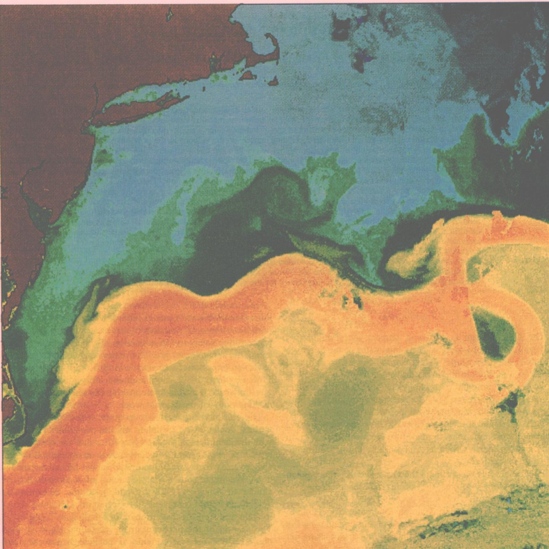
Figure 1: Satellite image of the Gulf Stream. Redder colors indicate warmer water. NOAA advanced very high resolution radiometer.

The main task of dynamical system’s theory in physical oceanography is to find and specify Lagrangian coherent structures and their impact on transport and mixing of water masses. Methods of that theory are attractive especially because they are common for different classes of models, dynamic and kinematic ones, and do not depend on their specific analytic forms because they use, mainly, fundamental geometric structures.

In this paper in the framework of the geometrical approach, we describe transport and mixing of passive particles in geophysical flows composed with the main Eulerian coherent structures in the ocean, a jet-like current and an eddy. The focus of this work is not on dynamics of the flow but rather on mechanisms of particle’s transport and mixing. That is why we use, as a prototype model, a kinematic model that was introduced in JTPL01 to describe the phenomenon of topographical eddies in the ocean K83 ; Z95 ; H73 ; GC97 . A current over seamounts and bottom cavities produce on the rotating Earth (quasi)stationary anticyclonic and cyclonic eddies, respectively. Such eddies may arise over underwater ridges and valleys as well.

In modeling oceanic flows we should take into account, generally speaking, a periodic tidal component of the current under consideration and a random component caused by turbulent diffusion. A simple stream function that is able to describe the main features of the two-dimensional flow of ideal fluid over a $\delta$-like bottom topography has the following normalized form:

$${\Psi=\ln{\sqrt{x^{2}+y^{2}}}+\varepsilon x+\xi x\left[(1-\alpha)\sin\tau+\alpha F(\tau)\right]},$$ (2)

where the first term represents a fixed point vortex placed at the point with Cartesian coordinates $x=y=0$, the second and third ones describe a steady and periodic components of the current with the normalized velocities $\varepsilon$ and $\xi$, respectively, and $F(\tau)$ is a random function with $\alpha$ being a normalized strength of noise.

II Geometry of transport and mixing in a periodically-driven flow: jet current with a tidal component over delta-like bottom topography

It immediately follows from incompressibility and two-dimensionality of the flow that equations of advection of passive particles are Hamiltonian ones

$$\dot{x} =u(x,y,\,\tau)=-\frac{\partial\Psi}{\partial y},$$ (3)

$$\dot{y} =v(x,y,\,\tau)=\frac{\partial\Psi}{\partial x},$$

where dot denotes differention with respect to the normalized time $\tau$. Analysis of transport and mixing of advected particles in the flow given by the stream function (2) without random force has been done in our papers PD04 ; JETP04 . In this section we discuss briefly the main results in the case of a periodic perturbation.

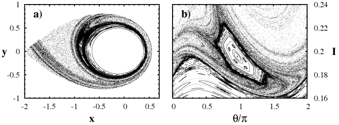
Figure 2: Poincaré sections of the mixing zone in the Cartesian (a) and the action-angle (b) coordinates.

In the absence of any time dependence in the streamfunction (2), the phase portrait of the unperturbed system consists of finite and infinite orbits separated by a separatrix encompassing the vortex and passing through the saddle point ($x=-1/\varepsilon$, $y=0$). In the polar coordinates ($x=\rho\cos\varphi$, $y=\rho\sin\varphi$), the unperturbed equations are solved in quadratures

$$\dot{\rho}=\pm\varepsilon\,\sqrt{1-\left(\frac{E-\ln\rho}{\varepsilon\rho}\right)^{2}},$$ (4)

where $E=\varepsilon\rho\cos\varphi+\ln\rho$ is an integral of motion. Depending on initial conditions, particles move either around the vortex along closed streamlines encompassed by the separatrix loop or around the loop along infinite streamlines. We have shown analytically and numerically in JTPL01 that under a small perturbation there exist transversal intersections of stable and unstable saddle-point manifolds in the neighborhood of the unperturbed separatrix. Under periodic perturbation, the particle’s trajectories deviate from the steady-flow streamlines. We define there zones in the phase (physical) space as follows: free-stream region (with incoming and outcoming components), mixing region and vortex core as the sets of trajectories with the number of times they wind around the vortex being zero, finite and infinite, respectively. Transport is trivial in the free-stream region. The size of the vortex core depends on the ratio $\varepsilon/\xi$. The vortex core consists of regular periodic and quasiperiodic trajectories with thin stochastic layers between them. As the value $\varepsilon/\xi$ increases, the vortex core grows while the mixing zone shrinks, correspondingly. The frequency of particle’s rotation in the vortex core depends on the distance from the singular point $(0,0)$ and is much higher than the perturbation frequency that is equal to $1$. Therefore, the perturbation can be treated as adiabatic with respect to most orbits inside the core, and these orbits are regular, except for those lying in a neighborhood of higher-order overlapping resonances which make up very narrow stochastic layers. In applications, it is important that KAM tori in the vortex core make up impermeable barriers that limit particle’s transport and mixing.

The topology of trajectories in the mixing zone is much more complicated. In Fig. 2 we show the Poincaré sections of the whole mixing region (Fig. 2a with Cartesian coordinates $x$ and $y$) and of a part of this region in the neighborhood of the half-integer primary resonance (Fig. 2b with the action $I$ and angle $\vartheta/\pi$ variables) which is surrounded by higher order resonances. High density of points around the vortex core and the islands means the presence of cantori there which can trap particles for a long time. The cantori should play an important role in transport and mixing of passive particles in geophysical flows.

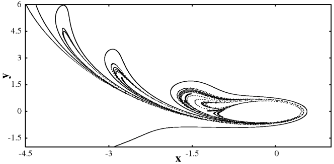
Figure 3: Image of the unstable manifold $\Lambda_{u}$ obtained as a snapshot of a dye streak at $\tau=15\pi$.

A chaotic invariant set $\Lambda$ is defined as a set of all orbits (except for the KAM tori and cantori) that never leave the mixing region. The set consists of an infinite number of periodic and aperiodic (chaotic) orbits. All orbits in this set are unstable. If a tracer belongs to $\Lambda$ at the initial moment, then it remains in the mixing region as $\tau\to\infty$ or $\tau\to-\infty$. The Poincaré section of $\Lambda$ is a set of points of Lebesgue measure zero. Most trajectories of the tracers advected in the mixing region of the incoming flow sooner or later leave the mixing region with the outgoing flow. However, their behavior is largely determined by the presence of $\Lambda$. They can “trail” after trajectories of the saddle set wandering in their neighborhoods.

Each orbit in the chaotic set and, therefore, the entire set $\Lambda$ have both stable and unstable manifolds. The stable manifold $\Lambda_{s}$ of the chaotic set is defined as the invariant set of orbits approaching those in $\Lambda$ as $\tau\to\infty$. The unstable manifold $\Lambda_{u}$ is defined as the stable manifold corresponding to time-reserved dynamics. Following trajectories in $\Lambda_{s}$, tracers, advected by the incoming flow, enter the mixing region and remain there forever. It was mentioned above that the corresponding initial conditions make up a set of measure zero. The tracer trajectories that are initially close to those in the chaotic set follow the chaotic-set trajectories for a long time and eventually deviate from them, and leave the mixing region along the unstable manifold. This behavior offers a unique opportunity to extract important properties of $\Lambda$ by measuring the characteristics of scattered particles and to observe unstable manifolds directly in laboratory experiments and even in geophysical flows.

An unstable manifold can be visualized by various methods. A blob consisting of many tracer particles, initially belonging to the intersection of the incoming flow with the stable manifold, spreads out and transforms into an intricate fractal curve approaching $\Lambda_{u}$ in the course of time. A similar pattern develops in dyeing experiments. The stable manifold lies in the coordinate-plane region bounded by the separatrix locations at the times corresponding to the two extrema reached during the perturbation period. This region extends to $-\infty$ along the $y$ axis, and its width is determined by the values of $\varepsilon$ and $\xi$. Only particles located in this region reach the mixing region. Figure  3 shows an image of the unstable manifold at $\tau=15\pi$ obtained numerically by integrating the equations of motions for particles continuously injected into the incoming flow at the point with $x_{0}=-4.357759744$ and $y_{0}=-6$. This pattern oscillates with the period of the flow. Tracer particles are advected along the fractal curve of the unstable manifold, which plays the role of an “attractor” in a Hamiltonian system JETP04 (there are no “classical” attractors in an incompressible flow).

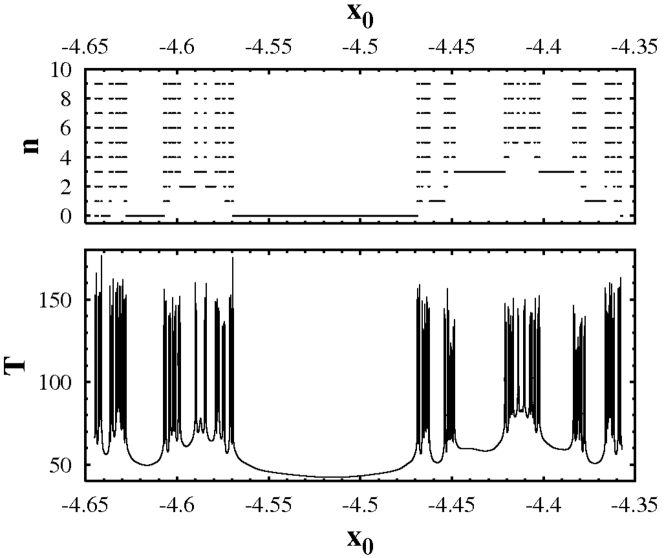
Figure 4: Advection fractal under a periodic perturbation. (a) the number of turns of particles around the vortex $n$ and (b) the respective exit time $T$ vs initial particle’s position $x_{0}$.

Choosing a material line in the incoming flow, we calculate the total number $n$ of turns executed by particles, belonging to this line, before they escape into the outgoing-flow region. The graph of $n(x_{0})$ is shown to be an intricate self-similar hierarchy of sequences of fragments of the material line (Fig. 4a). Their fractal properties are generated by the infinite sequence of intersections of stable and unstable manifolds with the material line segment as it rotates about the vortex. Following to the paper M03 , we refereed to the sequences of segments corresponding to each $n\geq 0$ as epistrophes. The epistrophes make up a hierarchy. Numerical experiments on epistrophes lying on different levels reveal the following trends: (I) each epistrophe converges to a limit point in the material line segment under consideration; (II) the end points of each segment in an $n$th-level epistrophe are the limit points of an $(n+1)$th-level epistrophe; (III) the lengths of segments in an epistrophe decrease in geometric progression; (IV) the common ratio $q$ of all progressions is related to the largest Lyapunov exponent for the saddle point as follows: $\lambda=-(1/2\pi)\ln q$. The epistrophic structure manifests itself in the plot of dependence of the time of exit of particles from the mixing zone $T$ on their initial positions in the material line $x_{0}$. This plot, shown in Fig. 4b, demonstrates wild oscillations of the exit time $T$ in the neighborhood of singular points of the Cantor-like set which, in principle, can be measured in real laboratory experiments.

Transport of passive particles is defined by a generic mechanism of scattering and folding in the flow, where stretching is caused by the stationary current component and folding — by the nonstationary tidal component and vortex. Strictly speaking, the structure of the fractal chaotic scattering is defined by the chaotic invariant set $\Lambda$ with a stable $\Lambda_{s}$ and an unstable $\Lambda_{u}$ manifolds. In the physical space $\Lambda_{s}$ acts as a variety of dynamical traps that are able to trap the particles for a while. We have identified a mechanism of trapping of the ends of strophes and epistrophes segments with the saddle unstable periodic orbit. Stable manifolds of the other unstable periodic and chaotic orbits “attract” advected particles and deposit in the structure of the fractal as well. Effect of different dynamical traps manifests itself on different timescales and for different values of the winding number $n$. For $\tau$ of the order of a few perturbation periods and small $n$, the mechanism of stretching and folding defines the particle’s transport. With increasing $\tau$ and $n$, the saddle orbit and other unstable periodic and chaotic orbits, belonging to the chaotic invariant set $\Lambda$, begin to play a significant role in forming the fractal.

II.1 Transport and mixing of tracers in a Woods Hole laboratory experiment

In this section we discuss the results of a laboratory experiment on chaotic advection which has been carried out at the Woods Hole oceanographic Institution DPH02 with the aim to find a possible mechanism for fluid transport and mixing among a western boundary current and subbasin recirculation gyres. Possible applications include the North Atlantic Deep Western Boundary Current and its adjacent mesoscale recirculation gyres. Transport and mixing of a dye in this real experiment are shown to be very similar to those in our model flow described in the preceding section. The respective flow has been set up in cylindrical laboratory tank (42.5 cm in diameter and a mean depth of 20 cm) with a slopping bottom (a slope is $s=0.15$). The tank rotates at a fixed rate $\Omega=2$ rad$\cdot$s^-1 and the circulation is driven by a lid that rotates at a differential rate $\Delta\Omega<0$, producing a uniform, anticyclonic surface stress vortex. Under a steady lid forcing, the (nearly) steady flow, consisting of the western boundary current with the velocity of $u_{\omega}\simeq 0.1\div 0.3$ cm$\cdot$s^-1 and the twin gyre, can be set up. The main control parameter in the experiment is the ratio between the Stommel and inertial boundary layers $\delta\simeq 8\sqrt{\Delta\Omega/\Omega}$.

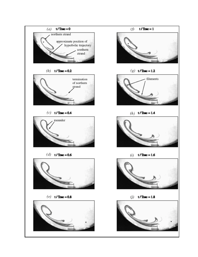
Figure 5: Evolution of dye lines over two forcing cycles in the Woods Hole laboratory experiment DPH02 .

The flow is almost steady if $\delta\leq 1.1$. Varying the lid rotation

$$\Delta(t)=\Delta\Omega_{0}\left(1+A_{\text{osc}}\sin\frac{2\pi t}{T_{\text{osc}}}\right),$$ (5)

it is possible to produce a time-periodic flow. Different methods have been used for visualizing and measuring the horizontal circulation. Neutrally buoyant plastic particles are suspended in the tank and illuminated by a laser light. Streak images showing the trajectories of the particles over short time intervals are made from digital video recording of the flow. Direct velocity measurements are made using particle image velocimetry with a spatial resolution of 1 cm. Another visualization technique involves the injection of dye into the flow using a needle. Dye patterns are illuminated from below and recorded from above using a video camera.

Within the range $1.1<\delta<1.4$, the recirculation splits into twin gyres, the northern and southern ones, forming the $\infty$-like figure. Mixing of the dye is weak in the steady regime and thought to be due to double diffusion between the salty ambient water and the food color dye. The time dependence introduces considerably more complicated mixing of the dye. The sequence in Fig. 5 DPH02 shows the evolution of the dye contour over two periods of the lid oscillation with $\delta=1.25$, $A_{\text{osc}}=0.05$ and $T_{\text{osc}}=131$ s. Dye is injected very close to the southern loop of unperturbed $\infty$-like separatrix (south is to the right and west is downward in the figure). Fig. 5a corresponds to the time moment about three cycles after injection is begun ($t/T_{\text{osc}}=0$), and Fig. 5j is for $t/T_{\text{osc}}=1.8$. In fact, the above pictures illustrate the evolution of the unstable manifold of the respective chaotic invariant set.

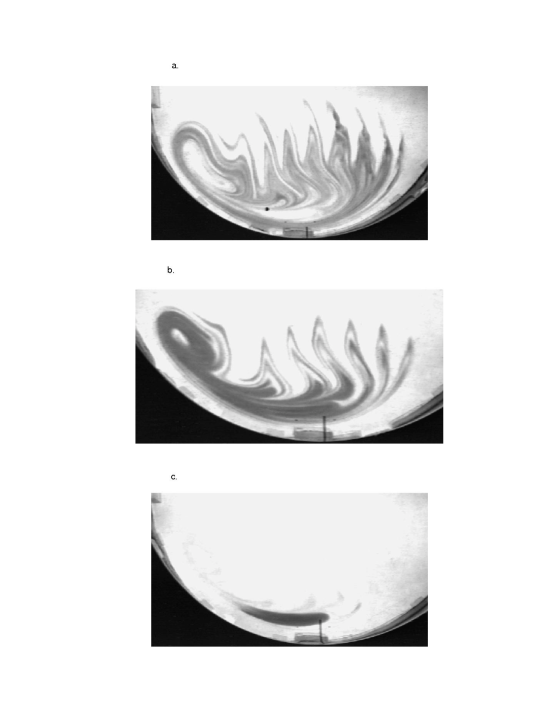
Figure 6: Dye patterns with different places of injection in the Woods Hole laboratory experiment DPH02 .

Transport and mixing depend strongly on which place in the flow the dye is injected. Fig. 6 DPH02 demonstrates the tracer streaklines with three different places of injection: just outside the southern gyre (Fig. 6a), just inside the western edge of the southern gyre (Fig. 6b) and inside the very center of the southern gyre (Fig. 6c). In the first two cases, the prominent filaments of the dye are seen both in the southern and northern gyres. That is because the dye is injected very close to the unperturbed separatrix in both the case. In the third case, the dye is injected inside the gyre core and remains confined there by KAM-tori which are impenetrable barriers for mixing (except for molecular diffusion).

We would like to pay attention on a similarity between the streaklines in our numerical experiment (Fig. 3) and the dye streaklines in the laboratory experiment (Fig. 6) DPH02 . In both the experiments, the dye is injected nearly the unperturbed separatrix, and both the pictures are images of the unstable manifolds of the respective chaotic invariant set $\Lambda$. A difference is that the unperturbed separatrix in our model flow is of a $\propto$-like form, and, therefore, our flow has only one gyre. The detailed analysis, of transport and mixing, similar to one that has been done in our papers PD04 ; JETP04 and in this paper, can be done for the laboratory flow DPH02 modeling transport and mixing of water masses among western boundary currents and subbasin recirculation gyres. Therefore, we expect for all the features of chaotic scattering: fractals, anomalous transport, stickiness, etc.

III Transport and mixing in a kinematic model of the current-eddy interaction in a noisy environment

III.1 Modeling noise

Real flows, of course, have noisy components due to environment. We will model noise $F(\tau)$ as a function consisting of a thousand of harmonics

$${F(\tau)=\frac{1}{\sqrt{N+1}}\sum\limits_{k=0}^{N}\sin(\omega_{k}\tau+\varphi_{k})},$$ (6)

with random phases $\varphi_{k}$ equally distributed in the range $[0:\,2\pi]$ and with frequencies $\omega_{k}=\omega_{b}+k(\omega_{e}-\omega_{b})/N$ equally distributed in a wide range between the lowest $(\omega_{b})$ and highest $(\omega_{e})$ frequencies. It is possible, in principle, to model the spectrum of an arbitrary form with the help of the series (6) introducing an amplitude factor depending on the frequency. Accordingly to the central limit theorem, $F(\tau)$ has a Gaussian distribution with zero expectation value because it is a large number of independent random variables. The factor $1/\sqrt{N+1}$ provides the variance to be equal to $1/2$.

Figure 7: A realization of the random function $F(\tau)$ with $\omega_{b}=2$, $\omega_{e}=5$ and $N=1000$.

Figure 8: PDF for the realization shown in Fig. 7 (circles). Gaussian distribution with $\sigma^{2}=1/2$ is shown by the solid line.

In Fig. 7 we show a piece of a realization of the function $F(\tau)$ and in Fig. 8 — a probability distribution for this realization. In simulation we use not the function $F(\tau)$ itself but its approximation by cubic splines providing the computation time to be almost independent on the number of harmonics of $F(\tau)$.

Modeling noise with the help of the series (6), instead of solving respective stochastic equations, has both the advantages and disadvantages. Among the advantages we mean the following:

• The function $F(\tau)$ is smooth. It allows to use in modeling equations with noise all the numerical methods and codes tested with problems without noise.

• Reproducibility. The function $F(\tau)$ depends on a set of phases $\varphi_{k}$ which is produced by a random-number generator. Initializing the generator with the same number, we reproduce the same realization of $F(\tau)$ under the same $\omega_{b}$, $\omega_{e}$ and $N$. In such a way we can do different numerical experiments with the same realization of noise.

• Independence of solutions on the integration step. In difference from numerical solving of stochastic equations with additional dependence on the integration step, our method does not contain any additional dependence on the integration step.

• Noise with an arbitrary spectrum can be modeled.

• A nonzero correlation length can be chosen to model noise with specific correlation properties.

The following disadvantages of our modeling of noise should be mentioned:

• It is necessary to cut the respective spectrum from above and below.

• Computing a high-frequency noisy perturbation requires more spline coefficients to memorize and more short integration steps.

• Spectrum of noise is not smooth but contains a large number of delta-like peaks.

III.2 Noise-induced transport and mixing

In this subsection we study transport and mixing of passive particles in a kinematic model inspired by the interaction of a jet current (like the Gulf Stream or the Kuroshio) with an eddy (see Fig. 1). Oversimplifying the problem, we model the respective flow by the stream function with a noisy component induced in the ocean by turbulence with different scales

$${\Psi_{noise}=\ln{\sqrt{x^{2}+y^{2}}}+\varepsilon x+\xi xF(\tau)}.$$ (7)

What is the effect of a broad-band weak noise on transport and mixing of passive particles? What happens with the main structures and properties of the flow — the vortex core, chaotic invariant set and its stable and unstable manifolds, fractals, anomalous transport, and main resonances — on reasonable timescales under a noisy-like excitation?

The most evident effect of noise is fussing of smooth invariant curves of a deterministic Hamiltonian system under consideration. In the limit $\tau\to\infty$, no regions in the phase space remain forbidden. Even a weak noise can induce transport of particles through KAM tori which cease to be impenetrable barriers to transport. Noise-induced diffusion depends mainly on the frequency range of noise and occurs on different time scales. For example, a vortex core may remain an impenetrable barrier for a long time comparing with a period of rotation of particles around the vortex.

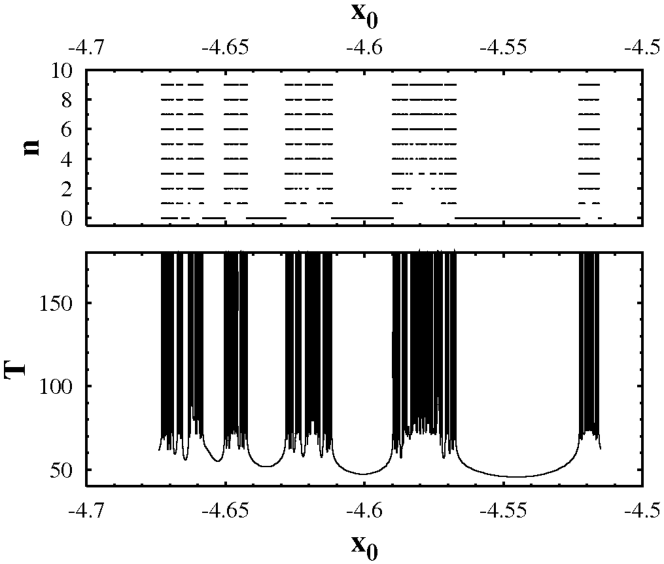
Figure 9: Advection fractal under a high-frequency noisy perturbation. (a) the number of turns of particles around the vortex $n$ and (b) the respective exit time $T$ vs initial particle’s position $x_{0}$.

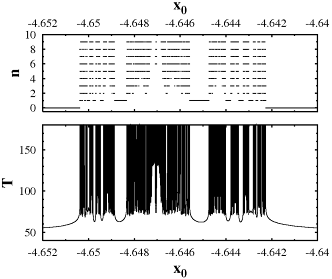
Figure 10: Magnification of one of the epistrophes of the fractal in Fig. 9.

Let us consider transport and mixing of particles chosen on the material line in the incoming flow with the coordinates $y_{0}=-6$, $x_{0}\in[-4.674:-4.515]$ under the influence of a steady current with the velocity $\varepsilon=0.5$ and a noise with the amplitude $\xi=0.1$ and the frequency range $\omega\in[2:5]$. We compute the dependencies of the number of turns of particles around the vortex $n$ and the respective exit times $T$ on the initial particle’s position. It follows from comparing Figs. 4 and 9, that a hierarchical fractal structure with epistrophes and strophes survives under a noisy excitation. Magnification of one of the epistrophes of the fractal in Fig. 9 demonstrates a self-similar structure (see Fig. 10). Distribution of exit times $T$ under the noisy perturbation (not shown there) demonstrates a more heavy tail and increasing values of the exit times comparing with the case of purely periodic perturbation PD04 . Noisy-induced breaking of deep invariant curves in the vortex core occurs due to numerous resonances between frequencies of the noise and the unperturbed frequencies. Therefore, a large number of particles may diffuse into the vortex core and stay there for a long time.

Figure 11: Semilogarithmic plot of the decrease in the segment length $L_{j}$ on its number $j$ in the zero-level epistrophe under high-frequency (circles) and low-frequency (squares) noisy perturbations.

The epistrophic law, found in the preceding section with the flow with a periodic perturbation, is valid under a noisy perturbation as well. In Fig. 11 we plot the dependencies of the segment lengths of the zero-level epistrophe on the number of the respective segment both for high-frequency ($\omega\in[2:5]$) and low-frequency ($\omega\in[0.4:1]$) noise. The exponential law is, in general, valid. We generalize the epistrophic law in the case of noise as follows:

$$q=\exp(-2\pi\lambda/\omega_{\text{eff}}),$$ (8)

where $\omega_{\text{eff}}$ is an effective frequency of perturbation defining the average frequency of appearing lobe-like structures with which particles quit the mixing zone. Whereas this frequency is exactly equal to unity in a periodic flow (see Fig. 3 with the lobe-like structures), it is equal to $\omega_{\text{eff}}\simeq 2.9$ under a high-frequency noisy perturbation and to $\omega_{\text{eff}}\simeq 0.3$ under a low-frequency one.

IV Noise-induced clustering of tracers

In geophysical field experiments one works mainly with single realizations of stochastic processes of interest and on a finite time interval $[0:T_{0}]$. By these reasons we can recover “deterministic” methods to explore the sets of stable trajectories satisfying to the condition of the finite-time invariance: if any set in the phase space at $t=0$ transforms to itself at $t=T_{0}$ without mixing, then it corresponds to an ensemble of trajectories which are stable by Lyapunov within the interval $[0:T_{0}]$. In order to find such stable sets for an arbitrary spectrum of perturbation, we propose the following map:

$${x_{n+1}=x(x_{n},y_{n},T_{0}),\qquad y_{n+1}=y(x_{n},y_{n},T_{0})},$$ (9)

where $x_{n}$ and $y_{n}$ are initial particle’s positions for the $n$-th iteration. In fact, this map is equivalent to a Poincaré map for a system under a periodic perturbation $\tilde{F}(\tau)$ consisting of identical pieces of $F(\tau)$ of the same duration $T_{0}$

$$\tilde{F}(\tau+mT_{0})=F(\tau),\quad 0\leq\tau\leq T_{0},\quad m=0,1,\dots.$$ (10)

In this way we replace our original randomly-driven system by a periodically-driven one. It should be emphasized that the validity of this replacement is restricted by the time interval $[0:T_{0}]$. By analogy with the usual Poincaré map, the key property of the map (9) is the following: each point of a continuous closed trajectory of the map (9) corresponds to a starting point of the solution of Eqs. (3) which remains stable by Lyapunov till the time $T_{0}$. The inverse statement is not, in general, true. It will be shown below that the map (9) provides sufficient but not necessary criterion of stability.

The phenomena, we report on in this section, is clustering of passive particles in a noisy flow resembling clustering of sound rays in an ocean underwater sound channel found in MUP04 . We have developed a special method to seek for such clusters, i. e. patches of tracers that move together for a long time in spite of action of a broad-band noise. Fig. 12a demonstrates the result of mapping with $T_{0}=2.3\pi$ on the configuration plane $(x,y)$, and Figs. 12b and c are magnification of the respective clusters in Fig. 12a. Prominent chains of the islands of stability can survive under a rather strong noisy perturbation ($\varepsilon=0.5$ and $\xi=0.1$) with the high-frequency range $\omega\in[9:10]$. To give a more direct manifestation of coherent clustering in a random flow that could be observed in real laboratory dye experiments, we compare the evolution of patches of particles chosen in the regions of stability and instability in the configuration space. In the upper panel in Fig. 13 we show the evolution of a coherent cluster corresponding to the small black point (the region of stability for a given realization of noise) with coordinates $x\simeq-0.535$ and $y\simeq 0.1$ in Fig. 12a. More or less compact evolution of this patch with $10^{4}$ particles goes on up to, at least, $\tau=6\pi$. For comparison, the lower panel in Fig. 13 demonstrates on the same time interval the evolution of the patch with the same number of particles chosen initially close to the coherent cluster at $\tau=0$. The respective initial patch is deformed strongly at $\tau=6\pi$.

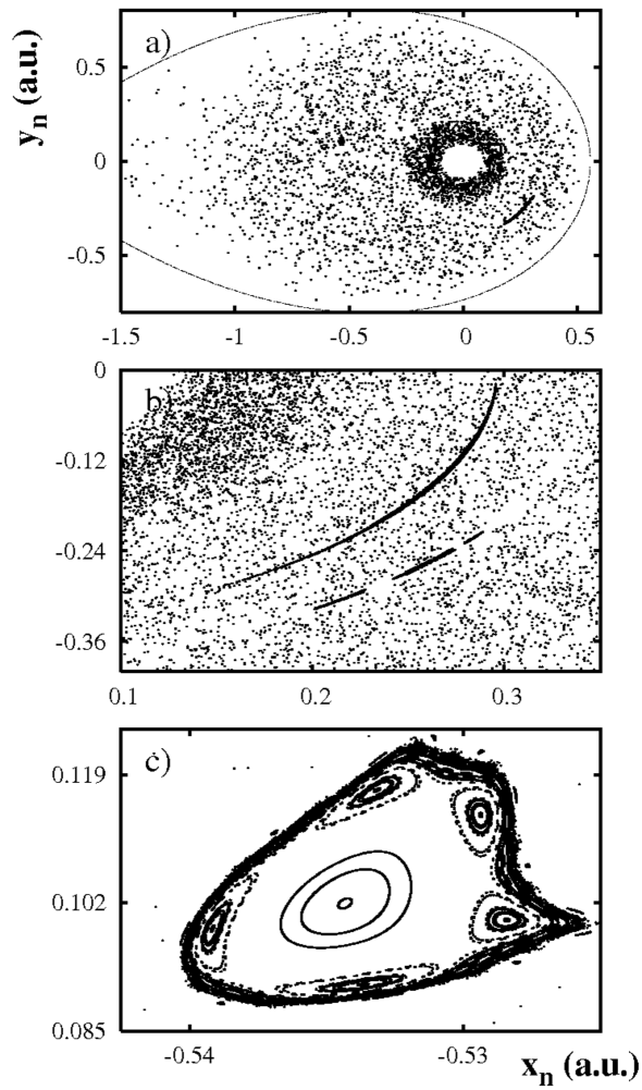
Figure 12: The map (9) with $T_{0}=2.3\pi$ revealing clusters of particles in a random velocity field with the amplitude $\xi=0.1$ and the frequency band $\omega\in[9:10]$. (a) general view in the phase plane $(x,y)$, (b) and (c) magnification of the respective clusters in (a). The dotted line is an unperturbed separatrix.

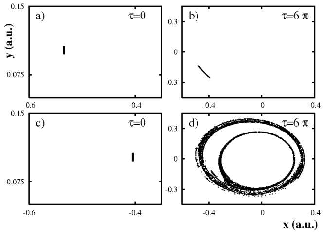
Figure 13: The compact evolution of a coherent cluster of particles (the upper panel) and deformation of an unstable patch of particles (the lower panel) in a random velocity field. Parameters of noise are given in caption to Fig. 12.

We would like to emphasize that the duration of the temporal interval $T_{0}$ in constructing the map (9) can be chosen arbitrarily. Thus, if $F(\tau)$ is a stationary random process, the regions of stability in the phase space exist at any time moment. The map (9) enables to prove definitely the existence of some regions of stability in the phase space but not all of them. Really, the map, constructed with any given value of $T_{0}$, can reveal only those stable sets which correspond to the phase oscillations nearby the fixed points of the map. However, there exist another regions of stability looking as chaotic ones on the map. The topology of the map changes with varying the mapping time $T_{0}$, and some regions in the phase space, which look as pseudochaotic on the map at $T_{0}=T_{1}$, become stable at $T_{0}=T_{2}>T_{1}$. The total area of the regions of stability, survived under a weak noise at $\tau=T_{0}$, can be estimated as an area of superposition of all the stable sets detected by the map (9) with the mapping step varying from $T_{0}$ to $T_{c}$, where $T_{c}$ is a mixing time.

Clustering in the ocean is a common feature that can be seen, for example, in satellite images of the ocean surface. In resent years new observation’s tools — quasi-Lagrangian current following floats and drifters — have been used to observe velocity field in the ocean at different levels of depth (for a review see D91 ). In connection with our numerical observation of coherent clusters of passive particles in the simple kinematic ocean model, we would like to pay attention to the results of the SOFAR floats program in the POLYMODE experiment in the North Atlantic RPW86 . Up to forty neutrally buoyant floats at $700$ m and $1300$ m were used to provide a quasi-Lagrangian description of the structure and evolution of the mesoscale eddy field. Those floats can be considered as quasi-passive tracers in a weak-noise environment. A large number of the deep floats revealed remarkably coherent motion over a two-month period.

V Conclusion

Kinematic models are attractive because of their simplicity, generality and possibility to reveal fundamental geometric structures responsible for Lagrangian transport and mixing in the ocean. In this paper we have reviewed transport and mixing of passive particles in a simple kinematic two-dimensional model with a topographical eddy and a tidal time-periodic current. We have found fractal features of transport and mixing in a kinematic model of the current-eddy interaction in a noisy environment and compared the results obtained with the purely deterministic case. The Lagrangian structures in our numerical experiments have been shown to be similar to those found in a recent laboratory dye experiment at Woods Hole DPH02 . We have demonstrated a non-trivial phenomenon of noise-induced clustering of passive particles and proposed a method to find the clusters in numerical experiments. These clusters are patches of advected particles which can move together in a random velocity field for comparatively long time. The clusters appear due to existence of regions of stability in the phase space which is the physical space in advection problems.

VI Acknowledgments

This work was supported by the Russia Government Program “World Ocean”, by the Program “Mathematical Methods in Nonlinear Dynamics” of the Russian Academy of Sciences, and by the Program for Basic Research of the Far Eastern Division of the Russian Academy of Sciences.

References

- (1) H.A. Dijkstra, Nonlinear physical oceanography, Dordrecht, Kluwer, 2000.
- (2) A.S. Bower, A simple kinematic mechanism for mixing fluid parcels across a meandering jet, J. Phys. Oceanogr. 21 (1989) 173-180.
- (3) J.Q. Duan, S. Wiggins, Fluid exchange across a meandering jet with quasi-periodic time variability, J. Phys. Oceanogr. 26 (1996) 1176-1188.
- (4) V.F. Kozlov, K.V. Koshel’, Barotropic model of chaotic advection in background flows, Izv. AN. Fiz. Atmos. Okean. 35 (1999) 137-144 [Izvestiya, Atmospheric and Oceanic Physics. 35 (1999) 123-130].
- (5) M. Budyansky, M. Uleysky, S. Prants, Hamiltonian fractals and chaotic scattering by a topographical vortex and an alternating current, Physica D. 195 (2004) 369-378.
- (6) L. Kuznetsov, C.K.R.T. Jones, M. Toner, Jr. A.D. Kirwan, Assessing coherent-feature kinematics in ocean models, Physica D. 191 (2004) 81-105.
- (7) Yu.G. Izrailsky, V.F. Kozlov, K.V. Koshel, Some specific features of chaotization of the pulsating barotropic flow over elliptic and axisymmetric sea-mounts, Phys. Fluids. 16 (2004) 3173-3190.
- (8) R.E. Davis, Lagrangian ocean studies, Annu. Rev. Fluid Mech. 23 (1991) 43-64.
- (9) T. Rossby, J. Price, D. Webb, The spatial and temporal evolution of a cluster of SOFAR floats in the POLYMODE local dynamics experiment (LDE), J. Phys. Oceanogr. 16 (1986) 428-442.
- (10) M.V. Budyansky, S.V. Prants, Universal mechanism of chaotic mixing in an elementary deterministic flow, Piśma Zh. Tekh. Fiz. 27 (2001) 51-56 [Tech. Phys. Lett. 27 (2001) 508-510].
- (11) V.F. Kozlov, Models of the Topographical Vortices in the Ocean, Nauka, Moscow, 1983 [in Russian].
- (12) V.N. Zyryanov, Topographical Vortices in Dynamics of Sea Currents, IVP RAN, Moscow, 1995 [in Russian].
- (13) N.G. Hogg, On the stratified Taylor columns, J. Fluid Mech. 58 (1973) 517-537.
- (14) D.R. Goldner, D.C. Chapman, Flow and particle motion induced above a tall seamount by steady and tidal background currents, Deep-Sea Research I. 44 (1997) 719-744.
- (15) M.V. Budyansky, M.Yu. Uleysky, S.V. Prants, Chaotic scattering, transport, and fractals in a simple hydrodynamic flow, Zh. Eksp. Teor. Fiz. 126 (2004) 1167-1179 [JETP. 99 (2004) 1018-1027].
- (16) K.A. Mitchell, J.P. Handley, B. Tighe, J.B. Delos and S.K. Knudson, Geometry and topology of escape, Chaos. 13 (2003) 880-891.
- (17) H.E. Deese, L.J. Pratt, K.R. Helfrich, A laboratory model of exchange and mixing between western boundary layers and subbasin recirculation gyres, J. Phys. Oceanogr. 32 (2002) 1870-1889.
- (18) D.V. Makarov, M.Yu. Uleysky, S.V. Prants, Ray chaos and ray clustering in underwater acoustics Chaos. 14 (2004) 79-95.