Regularization of moving boundaries in a Laplacian field
by a mixed Dirichlet-Neumann boundary condition — exact results

Abstract

The dynamics of ionization fronts that generate a conducting body, are in simplest approximation equivalent to viscous fingering without regularization. Going beyond this approximation, we suggest that ionization fronts can be modeled by a mixed Dirichlet-Neumann boundary condition. We derive exact uniformly propagating solutions of this problem in 2D and construct a single partial differential equation governing small perturbations of these solutions. For some parameter value, this equation can be solved analytically which shows that the uniformly propagating solution is linearly convectively stable.

Boundaries between two phases that move according to the gradient of a Laplacian or diffusive field, occur in many fields of the natural sciences and have a long and intricate research history Pelce ; well known examples include viscous fingering in Hele-Shaw flow st ; visfing , solidification fronts in under-cooled melts Pelce , migration of steps BCF or electromigration of voids electro0 ; electro on the surface of layered solids or boundaries of bacterial colonies in an external nutrition field bact . Viscous fingering here takes a paradigmatic role as the oldest and most studied problem — determining the long time dynamics up to today leads to mathematical surprises Tanveer ; Tanveer2 ; KL ; Jaume .

A similar moving boundary problem arises in so-called streamer discharges PREUWC ; PRLMan that precede sparks and lightning. Streamer ionization fronts can be understood as moving boundaries separating an ionized phase from a non-conducting phase PRLMan ; Man04 ; Bern1 . The inner front structure can be approximated by a boundary condition of mixed Dirichlet-Neumann-type, as we will sketch below. A similar boundary condition appears in step motion on the surface of layered solids when the Schwoebel barrier is taken into account BCF . Our boundary condition has a similar physical effect as the curvature correction in viscous fingering. We do show here that it indeed stabilizes certain uniformly translating shapes. In our analysis below, we encountered a number of surprises: $(i)$ planar fronts are linearly unstable to transversal perturbations of arbitrary wave vector $0<k<\infty$, still we find that sufficiently curved fronts are linearly convectively stable; $(ii)$ a simple explicit uniformly translating solution can always be found; $(iii)$ linear perturbations of these solutions can be reformulated in terms of a single partial differential equation, $(iv)$ if the solution of this perturbation problem is Taylor expanded and truncated at any finite order, the eigensolutions seem to be purely oscillating, $(v)$ however, for a particular parameter value, the linear perturbation theory has an explicit analytical solution that shows that there are no oscillations. Rather, perturbations might grow for some time, while they simultaneously are convected to the back where they disappear. Only a shift of the original shape remains for $t\to\infty$. To our knowledge, this is the first explicit solution showing the convective stabilization of a curved front according to the concept of Zeldovich comb .

In fact, the interfacial dynamics with our boundary condition can be addressed by explicit analysis much further than the classical viscous fingering problem. It therefore might contribute not only to the understanding of ionization fronts, but also shed new light on other moving boundary problems like the classical viscous fingering problem.

A simple moving boundary approximation for a streamer ionization front was suggested by Lozansky and Firsov Firsov : The front penetrates into a non-ionized and electrically neutral region (indicated with a ⁺) with a velocity determined by the local electric field ${\bf E}^{+}=-\nabla\varphi^{+}$:

$$\nabla^{2}\varphi^{+}=0~{},~{}~{}~{}v_{n}=\hat{\bf n}\cdot\nabla\varphi^{+},$$ (1)

where $\hat{\bf n}$ is the local normal on the boundary. Approximating the interior ionized region as ideally conducting

$$\varphi^{-}={\rm const.},$$ (2)

and the electric potential as continuous across the ionization boundary $\varphi^{+}=\varphi^{-}$, one arrives at the Lozansky-Firsov interfacial model. This model was suggested in PRLMan to explain streamer branching, and it was explicitly analyzed in Bern1 . Replacing the electric potential $\varphi$ by the pressure field $p$, one finds the non-regularized motion of viscous fingers in a Hele-Shaw cell. The model generically leads within finite time to the formation of cusps, i.e., of locations on the interface with vanishing radius of curvature entov .

We here propose to replace the boundary condition $\varphi^{+}-\varphi^{-}=0$ by

$$\varphi^{+}-\varphi^{-}=\epsilon\;\hat{\bf n}\cdot\nabla\varphi^{+}$$ (3)

to suppress these unphysical cusps. Here the length scale $\epsilon$ characterizes the width of the ionization front where the ionization increases and the electric field decreases. It determines the jump $\varphi^{+}-\varphi^{-}$ of the electric potential across the boundary for given field $\nabla\varphi^{+}$ ahead of the front.

The classical boundary condition for viscous fingering is $\varphi^{+}-\varphi^{-}=\gamma\kappa$ where $\kappa$ is the local curvature of the moving interface, and $\gamma$ is surface tension. In contrast, the boundary condition (3) does not involve front curvature, but can be derived from planar ionization fronts, more precisely from a minimal set of partial differential equations for electron and ion densities and their coupling to the electric field PREUWC . The formal derivation will be given elsewhere. Here we note that ignoring electron diffusion ($D=0$) as in Man04 , the planar uniformly translating front solutions of the p.d.e.s always yield a relation $\varphi^{+}-\varphi^{-}=F(\hat{\bf n}\cdot\nabla\varphi^{+})$. For large field $E^{+}=\hat{\bf n}\cdot\nabla\varphi^{+}$ ahead of the front, the function $F$ becomes linear, and the boundary condition (3) results.

This boundary condition has a similar physical effect as the curvature correction in viscous fingering: high local fields ahead of the front decrease due to the change of $\varphi^{+}$ on the boundary, and the interface moves slower than an equipotential interface (where $\varphi^{+}={\rm const}$). While the boundary condition of viscous fingering suppresses high interfacial curvatures that can lead to high fields, the boundary condition (3) suppresses high fields that frequently are due to high local curvatures. This physical consideration has motivated our present study whether the boundary condition (3) also regularizes the interfacial motion.

The minimal p.d.e. model for streamer fronts with $D=0$ leads to a dispersion relation with asymptotes

$$s(k)=\left\{\begin{array}[]{ll}vk&~{}~{}~{}\mbox{for }k\ll 1/\epsilon\\ v/\epsilon&~{}~{}~{}\mbox{for }k\gg 1/\epsilon\end{array}\right.$$ (4)

for linear transversal perturbations $e^{ikx+st}$ of planar interfaces Man04 . It is important to check whether the moving boundary approximation (1)–(3) reproduces this behavior. Indeed, analyzing planar interfaces we find $s(k)=vk/(1+\epsilon k)$ in full agreement with (4) as we will show in detail elsewhere. This strongly suggests that the interfacial model captures the correct physics. It shows furthermore, that planar fronts are linearly unstable against any wave-vector $k$ for all $\epsilon$.

We now restrict the analysis to the two-dimensional version of the model and to arbitrary closed streamer shapes in an electric field that becomes homogeneous

$$\varphi(x,y)\to-E_{0}x~{}~{}~{}\mbox{far from the ionized body}.$$ (5)

The problem is treated with conformal mapping methods Bern1 : The exterior of the streamer where $\nabla^{2}\varphi^{+}=0$ can be mapped onto the interior of the unit circle. Parameterizing the original space with $z=x+iy$ and the interior of the unit disk with $\omega$, the position of the streamer can be written as

$$z=x+iy=f_{t}(\omega)=\frac{1}{h_{t}(\omega)}=\sum_{k=-1}^{\infty}a_{k}(t)\;\omega^{k},$$ (6)

where $h_{t}(\omega)$ is analytical on the unit disk with a single zero at $\omega=0$ and therefore has the Laurent expansion given on the right. The boundary of the ionized body

$$\omega=e^{i\alpha},~{}~{}~{}\alpha\in[0,2\pi[,$$ (7)

is parametrized by the angle $\alpha$.

The potential $\varphi^{+}$ is a harmonic function due to (1), therefore one can find a complex potential $\Phi(z)=\varphi^{+}+i\psi$ that is analytic. Its asymptote is $\Phi(z)\to-E_{0}z$ for $|z|\to\infty$ according to (5). For the complex potential $\hat{\Phi}(\omega)$, this means that

$$\hat{\Phi}(\omega)=\Phi(f_{t}(\omega))=-E_{0}\;a_{-1}(t)\left(\frac{1}{\omega}+\sum_{k=0}^{\infty}c_{k}(t)\;\omega^{k}\right),$$ (8)

where the pole $\propto 1/\omega$ stems from the constant far field $E_{0}$, and the remainder is a Taylor expansion that accounts for the analyticity of $\hat{\Phi}$. The boundary motion $v_{n}=\hat{\bf n}\cdot\nabla\varphi$ (1) is rewritten as

$${\rm Re}\left[i\partial_{\alpha}f_{t}^{*}\;\partial_{t}f_{t}\right]={\rm Re}\left[-i\partial_{\alpha}\hat{\Phi}(e^{i\alpha})\right].$$ (9)

The boundary condition (3) takes the form

$${\rm Re}\left[\hat{\Phi}(e^{i\alpha})\right]=\epsilon\;{\rm Re}\left[\frac{i\partial_{\alpha}\hat{\Phi}(e^{i\alpha})}{|\partial_{\alpha}f_{t}|}\right].$$ (10)

The moving boundary problem is now reformulated as Eqs. (9) and (10) together with the ansätze (6) and (8) for $f_{t}$ and $\hat{\Phi}$.

For the unregularized problem (where $\epsilon=0$), it is well known that all ellipses with a main axis oriented parallel to the external field are uniformly translating solutions: for principal radii $r_{x,y}=a_{-1}\pm a_{1}$, they propagate with velocity $v=-E_{0}(r_{x}+r_{y})/r_{y}$, while the potential is $\hat{\Phi}=E_{0}a_{-1}(t)(\omega-1/\omega)$ Bern1 ; entov .

For a moving boundary problem with regularization, there are only rare cases where analytical solutions can be given, and frequently they are given only implicitly SolVF ; SolVF2 ; entov . For the present problem, however, an explicit solution is found for all $\epsilon>0$:

$$z = f_{t}(\omega)=\frac{a_{-1}}{\omega}+vt,~{}~{}~{}\partial_{t}a_{-1}=0,$$ (11)

$$\hat{\Phi}(\omega) = -E_{0}a_{-1}\left(\frac{1}{\omega}-\frac{1-\epsilon/a_{-1}}{1+\epsilon/a_{-1}}\;\omega\right).$$ (12)

This solution simply describes a circle $z=x+iy=a_{-1}e^{-i\alpha}+vt$ with radius $a_{-1}$ that according to (9) propagates with velocity $v=-2E_{0}/(1+\epsilon/a_{-1})$. Note that $\epsilon$ changes the velocity, but not the shape of the solution. Note further that the multiplicity of uniformly translating solutions reduces through regularization in a similar way as in viscous fingering, namely from a family of ellipse solutions characterized by two continuous parameters $a_{-1}$ and $a_{1}$ to a family of circle solutions characterized by only one radius $a_{-1}$ or interface width $\epsilon$.

The physical problem has two length scales, the interface width $\epsilon$ and the circle radius $a_{-1}$. In the sequel, we set $a_{-1}=1$, measuring all lengths relative to the radius of the circle.

Now the question arises whether a uniformly translating circle is stable against small perturbations, in particular, in view of the linear instability of the planar front (4). The basic equations (6)–(10) show a quite complicated structure, and it is a remarkable feature that linear stability analysis of the translating circle (11)–(12) can be reduced to solving a single partial differential equation. We write

$$f_{t}(\omega) = \frac{1}{\omega}+\tau+\beta(\omega,\tau),~{}~{}~{}\tau=vt,~{}~{}~{}v=\frac{-2E_{0}}{1+\epsilon},$$ (13)

$$\hat{\Phi}(\omega) = -E_{0}\left(\frac{1}{\omega}-\frac{1-\epsilon}{1+\epsilon}\;\omega\right)+v\;\phi(\omega,\tau),$$ (14)

where $\beta$ and $\phi$ are analytical in $\omega$ and assumed to be small. Eqs. (9) and (10) are expanded to first order in $\beta$ and $\phi$ about the uniformly translating circle and read

$${\rm Re}\left[\omega\;\partial_{\tau}\beta-\omega\partial_{\omega}\beta\right]={\rm Re}\left[-\omega\partial_{\omega}\phi\right]~{}~{}~{}\mbox{for }\omega=e^{i\alpha},$$ (15)

$$\frac{\epsilon}{2}\;\left(\omega+\frac{1}{\omega}\right){\rm Re}\left[\omega^{2}\partial_{\omega}\beta\right]={\rm Re}\left[\epsilon\;\omega\partial_{\omega}\phi+\phi\right].$$ (16)

By construction, $F(\omega)=\partial_{\tau}\beta-\partial_{\omega}\beta+\partial_{\omega}\phi$ is analytical for $|\omega|<1$, and Eq. (15) shows that ${\rm Re}[\omega\;F(\omega)]=0$ for $|\omega|=1$. Furthermore, it is clear that $\omega\;F(\omega)$ vanishes for $\omega=0$. Therefore,

$$0=\omega\;F(\omega)=\omega\;\left(\partial_{\tau}\beta-\partial_{\omega}\beta+\partial_{\omega}\phi\right)$$ (17)

is valid on the whole closed unit disk. The corresponding analysis of Eq. (16) yields

$$\frac{\epsilon}{2}\;\left(\omega+\frac{1}{\omega}\right)\;\omega^{2}\partial_{\omega}\beta=\epsilon\omega\partial_{\omega}\phi+\phi+{\rm const.}$$ (18)

To this equation the operator $\omega\partial_{\omega}$ is applied, and Eq. (17) is used to eliminate terms containing $\omega\partial_{\omega}\phi$. As a result, we find an equation only for the function $\beta(\omega,\tau)$:

$${\cal L}_{\epsilon}\;\beta = 0,$$ (19)

$${\cal L}_{\epsilon} = -\epsilon\;(1-\omega^{2})\;\omega\;\partial_{\omega}^{2}-(2+\epsilon-3\epsilon\;\omega^{2})\;\partial_{\omega}$$ (20)

$$\qquad\qquad+2\epsilon\;\omega\partial_{\omega}\;\partial_{\tau}+2(1+\epsilon)\;\partial_{\tau}.$$

Eq. (19) has to be solved for arbitrary initial conditions $\beta(\omega,0)$ that are analytical in some neighborhood of the unit disk. The operator ${\cal L}_{\epsilon}$ conserves analyticity in time. $\epsilon$ is a singular perturbation that multiplies the highest derivatives $\partial_{\omega}^{2}$ and $\partial_{\omega}\partial_{\tau}$.

The case $\epsilon=0$ is almost trivial, since ${\cal L}_{\epsilon}$ reduces to

$${\cal L}_{0}=2\;(\partial_{\tau}-\partial_{\omega}).$$ (21)

Thus all solutions can be written as

$$\beta(\omega,\tau)=\hat{\beta}(\omega+\tau),$$ (22)

where $\hat{\beta}(\zeta)$ is any function analytic in a neighborhood of the unit disk $|\zeta|\leq 1$. The time evolution just amounts to a translation along the strip $-1\leq{\rm Re}~{}\zeta\leq\infty$, $|{\rm Im}~{}\zeta|\leq 1$. Any singularity of $\hat{\beta}$ at some finite point $\zeta$ on the strip will lead to a breakdown of perturbation theory within finite time; this is the generic behavior as found previously in the full nonlinear analysis of this unregularized problem. Of course, there also exist solutions that stay bounded for all times.

A different perspective on $\epsilon=0$ is that the Richardson moments are an infinite sequence of conserved quantities entov . A reflection of this property is that any polynomial $\beta(\omega,\tau)=\sum_{k=0}^{N}b_{k}(\tau)\omega^{k}$ for any $N$ with an appropriate choice of the time dependent functions $b_{k}(\tau)$ is an exact solution for all times $\tau>0$, for linear perturbation theory (19) as well as for the full nonlinear problem Bern1 , i.e., any truncation of the Laurent series (6) leads to exact solutions.

This observation suggests that an expansion in powers of $\omega$ is a natural ansatz also for nonvanishing (but small) $\epsilon$. Taking as initial condition some polynomial of order $N$, one finds from the form (20) of ${\cal L}_{\epsilon}$ that higher modes $\omega^{k}$, $k>N$ are generated dynamically — similarly to the daughter singularities in regularized viscous fingers Tanveer . When the expansion in $\omega$ is truncated at some arbitrary $N^{\prime}$, it can be shown that the problem for any truncation $N^{\prime}$ and for any value $\epsilon>0$ has purely imaginary temporal eigenvalues. One would therefore expect all eigensolutions for $\epsilon>0$ to be purely oscillating in time. However, this behavior seems inconsistent with our exact solution for $\epsilon=1$.

For $\epsilon=1$ it turns out that the operator factorizes

$${\cal L}_{1} = \Big{[}2\partial_{\tau}-(1-\omega^{2})\partial_{\omega}\Big{]}\;\Big{[}2+\omega\partial_{\omega}\Big{]}.$$ (23)

which allows us to construct the general solution. We introduce the function

$$g(\omega,\tau)=[2+\omega\partial_{\omega}]\;\beta(\omega,\tau),$$ (24)

that obeys the equation

$$[2\partial_{\tau}-(1-\omega^{2})\partial_{\omega}]\;g(\omega,\tau)=0.$$ (25)

The general solution of this equation reads

$$g(\omega,\tau)=G\left(\frac{\omega+T}{1+T\omega}\right),~{}~{}~{}T=\tanh\frac{\tau}{2}.$$ (26)

The function $G$ is derived from the initial condition as

$$G(\omega)=g(\omega,0)=[2+\omega\partial_{\omega}]\;\beta(\omega,0);$$ (27)

hence it is analytical in a neighborhood of the unit disk. Finally, Eq. (24) is solved by

$$\beta(\omega,\tau)=\int_{0}^{\omega}\frac{x\;dx}{\omega^{2}}\;G\left(\frac{x+T}{1+Tx}\right).$$ (28)

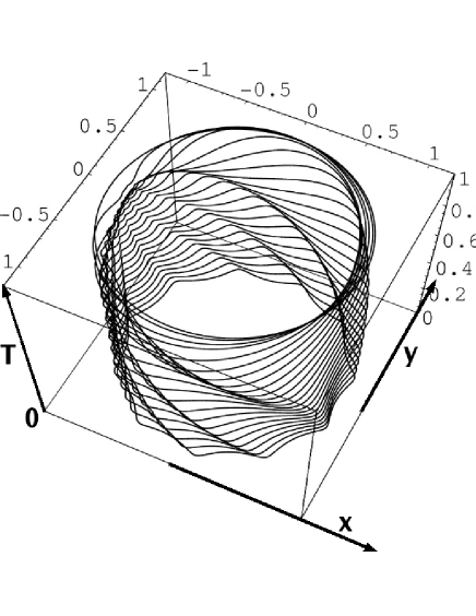
Figure 1: Temporal evolution of a perturbed circle $f_{t}(\omega)-\tau=1/\omega+\beta(\omega,\tau)$ moving in the positive $x$-direction, according to Eqs. (12) and (26)–(28). The constant motion in time $\tau$ is subtracted. The initial perturbation is a Fourier mode $\beta(\omega,0)=-0.5\;\omega^{k}/(k+2)$ with $k=10$. The evolution during times $0\leq\tau\leq\infty$ corresponding to $0\leq T\leq 1$ is shown for time steps $T=$ 0, 0.05, 0.1, $\ldots$, 0.85, 0.9, 0.95, 0.97, 0.99, 1.0.

Now the one parameter family of mappings

$$\omega\longrightarrow\zeta_{T}(\omega)=\frac{\omega+T}{1+T\omega},~{}~{}~{}-1<T<1,$$ (29)

forms a subgroup of the automorphisms of the unit disk. Thus on the level of $G(\zeta)$, the dynamics amounts to a conformal mapping of the unit disk $|\omega|\leq 1$ onto itself. This dynamics is somewhat distorted by the additional integration (28) leading to $\beta(\omega,\tau)$, but it is easily seen that $\beta(\omega,\tau)$ and $\partial_{\omega}\beta(\omega,\tau)$ are bounded uniformly in $\tau$ for $|\omega|\leq 1$. Hence, contrary to the unregularized problem for $\epsilon=0$, only perturbations contribute that are bounded for all times. Hence an infinitesimal perturbation can never form cusps. Furthermore, the mapping $\omega\to\zeta_{T}(\omega)$ has fixed points $\omega=\pm 1$; and for $\tau\to\infty$, i.e., $T\to 1$, it degenerates to $\zeta_{1}(\omega)\equiv 1$, provided $\omega\neq-1$. We thus find the asymptotic behavior

$$\beta(\omega,\tau)\stackrel{{\scriptstyle\tau\to\infty}}{{\longrightarrow}}\frac{G(1)}{2},$$ (30)

independent of $\omega$ for any initial condition. Therefore asymptotically, the perturbation just shifts the basic circular solution without change of shape. Indeed, it is easily checked that any pronounced structure of the initial perturbation that is not located right at the top at $\omega=1$, is convected with increasing time toward $\omega=-1$ where it vanishes. This is an outflow of the simple dynamics of $G(\zeta)$ as pointed out above. Fig. 1 illustrates this behavior.

To summarize, we have found that the boundary condition (3) at least for $\epsilon=1$ regularizes our problem in the sense that an infinitesimal perturbation of a uniformly translating circle stays infinitesimal for all times and vanishes asymptotically for $\tau\to\infty$ up to an infinitesimal shift of the complete circle. This statement is based on an exact analytical solution for an arbitrary initial perturbation. At the present stage, we have indications that this behavior of infinitesimal perturbations is generic for $\epsilon>0$, while the solution is unstable for $\epsilon=0$. Furthermore, we expect that the convection of perturbations to the back of the structure applies similarly for other shapes like fingers. When applying the present calculation to streamers, we in fact have to assume this to be true, since streamers are typically not closed bodies, but rather the tips of ionized channels. Finally, the behavior of finite perturbations and their nonlinear analysis will require future investigations.

References

- (1) P. Pelcé, Dynamics of curved fronts, review and collection of papers, Academic Press (Boston, 1988).
- (2) P.G. Saffman, G.I. Taylor, Proc. Roy. Soc. London, Series A, 245, 312 (1958).
- (3) D. Bensimon, L.P. Kadanoff, S. Liang, B.I. Shraiman, and C. Tang, Rev. Mod. Phys. 58, 977 (1986).
- (4) P. Politi et al., Phys. Rep. 324, 271 (2000).
- (5) M. Ben Amar, Physica D 134, 275 (1999).
- (6) P. Kuhn, J. Krug, F. Hausser, A. Voigt, Phys. Rev. Lett. 94, 166105 (2005).
- (7) J. Müller, W. van Saarloos, Phys. Rev. E 65, 061111 (2002).
- (8) M. Siegel, S. Tanveer, Phys. Rev. Lett. 76, 419 (1996).
- (9) S. Tanveer, J. Fluid Mech. 409, 273 (2000).
- (10) D.A. Kessler, H. Levine, Phys. Rev. Lett. 86, 4532 (2001).
- (11) J. Casademunt, Chaos 14, 809 (2004).
- (12) U. Ebert, W. van Saarloos, C. Caroli, Phys. Rev. E 55, 1530 (1997).
- (13) M. Arrayás, U. Ebert, W. Hundsdorfer, Phys. Rev. Lett. 88, 174502 (2002).
- (14) M. Arrayás, U. Ebert, Phys. Rev. E 69, 036214 (2004).
- (15) B. Meulenbroek, A. Rocco, U. Ebert, Phys. Rev. E 69, 067402 (2004).
- (16) Ya.B. Zel’dovich, A.G. Istratov, N.I. Kidin, V.B. Librovich, Combustion Sci. and Techn. 24, 1 (1980).
- (17) E.D. Lozansky and O.B. Firsov, J. Phys. D: Appl. Phys. 6, 976 (1973).
- (18) V.M. Entov, P.I. Etingof and D.Ya. Kleinbock, Eur. J. Appl. Math. 4, 97 (1993).
- (19) G.L. Vasconcelos, L.P. Kadanoff, Phys. Rev. A 44, 6490 (1991).
- (20) D. Crowdy, J. Fluid Mech. 409, 223 (2000).