Systematic Density Expansion of the Lyapunov Exponents for a Two-dimensional Random Lorentz Gas

Abstract

We study the Lyapunov exponents of a two-dimensional, random Lorentz gas at low density. The positive Lyapunov exponent may be obtained either by a direct analysis of the dynamics, or by the use of kinetic theory methods. To leading orders in the density of scatterers it is of the form $A_{0}\tilde{n}\ln\tilde{n}+B_{0}\tilde{n}$, where $A_{0}$ and $B_{0}$ are known constants and $\tilde{n}$ is the number density of scatterers expressed in dimensionless units. In this paper, we find that through order $(\tilde{n}^{2})$, the positive Lyapunov exponent is of the form $A_{0}\tilde{n}\ln\tilde{n}+B_{0}\tilde{n}+A_{1}\tilde{n}^{2}\ln\tilde{n}+B_{1}\tilde{n}^{2}$. Explicit numerical values of the new constants $A_{1}$ and $B_{1}$ are obtained by means of a systematic analysis. This takes into account, up to $O(\tilde{n}^{2})$, the effects of all possible trajectories in two versions of the model; in one version overlapping scatterer configurations are allowed and in the other they are not.

Keywords: Lyapunov exponent, Lorentz gas, density expansion.

I Introduction

The Lorentz gas is a model consisting of a set of scatterers that are fixed in space, together with a moving point particle (or a cloud of mutually non-interacting point-particles) undergoing collisions with the scatterers. Here we will consider two variants of the two-dimensional version, where the scatterers are fixed hard disks, placed at random in the plane and the collisions of the point particle with the scatterers are elastic and specular. In the first version the positions of the scatterers are completely random, so different scatterers may overlap each other (this corresponds to the case of point scatterers with a moving particle of circular shape). In the second version the scatterers may not overlap each other, but each configuration satisfying this constraint has equal a priori weight (this corresponds to a hard-sphere interaction between the scatterers). The Lorentz Gas has proved to be very useful for studying the general relations existing between dynamical systems theory and the non-equilibrium properties of many body systems. Explicit examples of such relationships encompass the escape rate formalism of Gaspard and Nicolis GasNic ; D_cup_book as well as the Gaussian thermostat formalism developed by Evans and co-workers gaussEv ; D_cup_book and by Hoover and co-workers gaussHoov ; D_cup_book . The Lorentz gas is known to be chaotic due to the convex shape of the boundaries of the scatterers. Its chaotic properties can be analyzed in fair detail, at least if the system is sufficiently dilute, in other words, the average distance between neighboring scatterers is large compared to their radius. For the model where the scatterers are placed on a periodic lattice (the Sinai billiard) Sinai has shown mixing and ergodicity Sinai_rms_70 and demonstrated that on large time and length scales the motion of the point particle is diffusive commentSinai . Already much earlier Krylov Krylov_book_pup conjectured that to leading order the positive Lyapunov exponent is of the form $\tilde{n}\ln\tilde{n}$, with $\tilde{n}\equiv na^{2}$ proportional to the density of scatterers. Subsequently Van Beijeren et al. vBD_prl_95 ; vBD_prl_96 ; vBLD_pre_98 carried out kinetic theory calculations yielding explicit expressions for the Lyapunov exponents of a disordered Lorentz gas (random configuration of scatterers) to leading orders, i.e. up to $O(\tilde{n})$ in the scatterer density. These studies confirmed Krylov’s conjecture and provided explicit values for the constants $A_{0}$ and $B_{0}$ appearing in the leading terms $A_{0}\tilde{n}\ln\tilde{n}+B_{0}\tilde{n}$ of the expansion of the largest Lyapunov exponent in terms of the scatterer density. The kinetic theory methods used for obtaining this result, employ an averaging over all allowed configurations of the scatterers.

Up to quadratic order in the density of scatterers, the positive Lyapunov exponent can be calculated by similar kinetic theory methods, refining the averaging procedure described above, such that it (i) takes into account the effects of non-overlap of the scatterers (for the non-overlapping scatterer model) and (ii) accounts for the most important effects of correlated collisions. The additional contributions to the positive Lyapunov exponent resulting from (i) and (ii) yield the positive Lyapunov exponent correct through order $\tilde{n}^{2}$. The purpose of this paper is to present a systematic  analysis to calculate these additional contributions and to give explicit values for the new coefficients appearing in the expression $A_{0}\tilde{n}\ln\tilde{n}+B_{0}\tilde{n}+A_{1}\tilde{n}^{2}\ln\tilde{n}+B_{1}\tilde{n}^{2}$ for the positive Lyapunov exponent up to this order. This is done in two steps: in the first step, we calculate the positive Lyapunov exponent up to $O(\tilde{n}^{2})$, assuming that the collisions between the point particle with the scatterers are uncorrelated. This embodies that the particle does not encounter any scatterer more than once, plus that all previous knowledge on the presence and absence of scatterers on the track of the point particle is ignored. However, in the non-overlapping scatterer model the influence of the non-overlap condition on the collision frequency is taken into account (for the overlapping model no corrections are needed for this at the given orders in $\tilde{n}$). In the second step, we consider (ii), and calculate corrections to the Lyapunov exponents due to correlated collision sequences in which the point particle either encounters the same scatterer more than once, or its scattering probability is enhanced or suppressed by the knowledge resulting from previous collisions, or the absence thereof. This includes the immediate suppression of collisions as result of the non-overlap condition.

The structure of this paper is as follows: in Sec. II, we briefly discuss the general theory of the Lyapunov exponents for a two-dimensional, random Lorentz gas. In Sec. III, we calculate the Lyapunov exponents through $O(\tilde{n}^{2})$ and obtain the constants $A_{1}$ and $B_{1}$, defined above. We conclude the paper with some discussions in Sec. IV. We note here that the structure of the calculation presented in this paper is based on a thorough and intricate mathematical formalism, which is summarized in the Appendix.

II Lyapunov exponents of the random Lorentz gas in two dimensions: General Theory

The random Lorentz gas consists of point particles of mass $m$, moving among a random array of fixed scatterers. In two dimensions, the scatterers are hard disks of radius $a$. We will consider two versions of the model: the Lorentz gas with overlapping scatterers, in which each configuration of scatterers a priori has equal probability (hence no weighting according to the amount of free volume left to the point particles!), and the Lorentz gas with non-overlapping scatterers, in which scatterers cannot overlap each other, but each configuration of scatterers satisfying this constraint a priori is equally likely. For a system with $N$ scatterers in a two-dimensional volume $V$ the number density of scatterers is $n=N/V$, and at low density $\tilde{n}\ll 1$. There is no interaction between point particles. These particles, therefore, travel freely during flights between collisions with the scatterers. The collisions between a point particle and a scatterer are instantaneous, specular and elastic. During flights, the equations of motion of a point particle are

$$\dot{{\bm{r}}}\,=\,{{\bm{v}}}\,=\,\frac{{\bm{p}}}{m},{\hskip 28.45274pt}\dot{{\bm{p}}}\,=\,m\dot{{\bm{v}}}\,=\,0\,.$$ (1)

At a collision with a scatterer, the post-collisional position and velocity, ${\bm{r}}_{+}$ and ${\bm{v}}_{+}$ of the point particle are related to its pre-collisional position and velocity, ${\bm{r}}_{-}$ and ${\bm{v}}_{-}$, by

$${\bm{r}}_{+}\,=\,{\bm{r}}_{-}\,,{\hskip 28.45274pt}{\bm{v}}_{+}\,=\,{\bm{v}}_{-}\,-\,2\,({\bm{v}}_{-}\cdot\hat{\bm{\sigma}})\,\hat{\bm{\sigma}}\,.$$ (2)

Here $\hat{\bm{\sigma}}$ is the unit vector in the direction from the center of the scatterer to the point of collision (see Fig. 1). Notice that the dynamics generated by Eqs. (1-2) keep the speed of the point particle constant at $v$. The instantaneous velocity direction of the particle is given by $\hat{\bm{v}}(t)={\bm{v}}(t)/v$.

Figure 1: Collision between a point particle and a scatterer.

The Lorentz gas with circular scatterers is a hyperbolic dynamical system. Due to the convex nature of the collisions with the scatterers, typically, the distance between two infinitesimally close trajectories in phase space, $[{\bm{r}}(t),{\bm{v}}(t)]$ and $[{\bm{r}}+\delta{\bm{r}}(t),{\bm{v}}(t)+\delta{\bm{v}}(t)]$, increases exponentially with time. There are two non-zero Lyapunov exponents, which sum to zero. We denote the positive Lyapunov exponent by $\lambda_{+}$. Without any loss of generality, one can characterize the time evolution of the separation between two nearby trajectories by that of its projection onto ${\bm{v}}$-space. The positive Lyapunov exponent then can be defined as

$$\lambda_{+}\,=\,\lim_{T\rightarrow\infty}\,\lim_{|\delta{\bm{v}}(t_{0})|\rightarrow 0}\,\frac{1}{T}\,\ln\,\frac{|\delta{{\bm{v}}}(t_{0}\,+\,T)|}{|\delta{{\bm{v}}}(t_{0})|}\,.$$ (3)

The non-overlapping random Lorentz gas is generally supposed to be ergodic, even in the infinite-system limit (although we do not know of any proof of this). Therefore this definition of $\lambda_{+}$ should be (almost) independent of the choice of the initial point of the trajectory. For the overlapping Lorentz gas the situation is slightly more subtle: in this model, if the volume becomes large enough, ergodicity will be broken. There will always be finite enclosures formed by three or more scatterers, from which a point particle cannot escape if it is trapped inside initially (see Fig. 2). However, as long as the density of scatterers is below a critical percolation density, in the infinite system limit there will always be a single unbounded percolating region on which the motion of the point particles is diffusive on large time and length scales. We will be interested in the Lyapunov exponents of such particles only (even though particles moving inside an enclosure will also exhibit a positive Lyapunov exponent).

Figure 2: A situation for the Lorentz gas with overlapping scatterers, wherein the point particle cannot leave the enclosure formed by the four scatterers.

As an alternative to Eq. (3), one can also choose to measure the separation of two nearby trajectories in ${\bm{r}}$-space — after all, $\delta{\bm{v}}(t)=\displaystyle{\frac{d\delta{\bm{r}}(t)}{dt}}$. In this representation the positive Lyapunov exponent becomes

$$\lambda_{+}\,=\,\lim_{T\rightarrow\infty}\,\lim_{|\delta{\bm{r}}(t_{0})|\rightarrow 0}\,\frac{1}{T}\,\ln\,\frac{|\delta{{\bm{r}}}(t_{0}\,+\,T)|}{|\delta{{\bm{r}}}(t_{0})|}\,.$$ (4)

When calculating $\lambda_{+}$ using Eq. (3), one may take advantage of the feature that the separation in velocity space between the two trajectories undergoes a change only  at the collisions with the scatterers. If the point particle suffers $k$ collisions between time $t_{0}$ and $t_{0}+T$, then vBLD_pre_98

$$\lambda_{+}\,=\,\lim_{T\rightarrow\infty}\,\lim_{|\delta{\bm{v}}(t_{0})|\rightarrow 0}\,\frac{k}{T}\,\frac{1}{k}\,\sum_{i=1}^{k}\ln\frac{|\delta{\bm{v}}_{i+}|}{|\delta{\bm{v}}_{i-}|}\,,$$ (5)

where, $\delta{\bm{v}}_{i-}$ and $\delta{\bm{v}}_{i+}$ are respectively the pre- and the post-collisional separation in velocity space between the two trajectories at the $i$-th collision.

On the other hand, to obtain the time evolution of $|\delta{{\bm{r}}}(t)|$, one may introduce another dynamical quantity, called the radius of curvature, and defined as $\rho=v\displaystyle{\frac{|\delta{\bm{r}}(t)-\hat{\bm{v}}(t)\cdot\delta{\bm{r}}(t)|}{|\delta{\bm{v}}(t)-\hat{\bm{v}}(t)\cdot\delta{\bm{v}}(t)|}}$ vBD_prl_95 ; vBLD_pre_98 ; D_cup_book . It characterizes the divergence between neighboring trajectories and in two dimensions it may be defined as the distance of the actual positions on a pair of such trajectories to their mutual intersection point (with $\rho$ positive if this point is found in the past). In terms of the radius of curvature the positive Lyapunov exponent may be expressed as Sinai_rms_70 ,

$$\lambda_{+}\,=\,\lim_{T\rightarrow\infty}\,\frac{v}{T}\int_{t_{0}}^{t_{0}\,+\,T}\,\frac{d\,t}{\rho(t)}.$$ (6)

During a free flight, the equation of motion for $\rho$ is given by D_cup_book

$$\dot{\rho}\,=\,v\,.$$ (7)

At a collision with a scatterer, the post-collisional radius of curvature $\rho_{+}$ is related to the pre-collisional radius of curvature $\rho_{-}$ by vBD_prl_95 ; vBLD_pre_98 ; D_cup_book :

$$\frac{1}{\rho_{+}}\,=\,\frac{1}{\rho_{-}}\,+\,\frac{2}{a\cos\phi}\,,$$ (8)

which is well-known from geometric optics. Here $\phi$ is the collision angle, i.e, $\cos\phi\,=\,|\hat{\bm{v}}_{-}\cdot\hat{\bm{\sigma}}|\,=\,|\hat{\bm{v}}_{+}\cdot\hat{\bm{\sigma}}|$ (see Fig. 1). Equations (7) and (8), for a given initial condition $[{\bm{r}}(t_{0}),{\bm{v}}(t_{0})]$ and a fixed spatial arrangement of the scatterers, can be solved together to obtain $\rho(t)$ as a function of ${\bm{r}}(t_{0})$ and ${\bm{v}}(t_{0})$. Consider a set of trajectory pairs generated from the same reference trajectory by starting tangent trajectories with $\delta{\bm{r}}(t_{0})=0$ and $\delta{\bm{v}}(t_{0})=\delta{\bm{v}}_{0}$ at a range of initial times $t_{0}$. One easily convinces oneself that the radius of curvature along the trajectory rapidly approaches a limiting value, $\rho({\bm{r}},{\bm{v}})=\lim_{t_{0}\rightarrow-\infty}\rho({\bm{r}},{\bm{v}},t_{0})$, with $\rho({\bm{r}},{\bm{v}},t_{0})$ the radius of curvature at the phase point $({\bm{r}},{\bm{v}})$ for a trajectory bundle starting out from $[{\bm{r}}(t_{0}),{\bm{v}}(t_{0})]$. Combining Eqs. (7) and (8) one finds that as a function of decreasing $t_{0}$ $\rho({\bm{r}},{\bm{v}},t_{0})$ can be expressed as a rapidly converging continued fraction. In Eq. (6) $\rho(t)$ therefore can be replaced by $\rho({\bm{r}}(t),{\bm{v}}(t))$, independent of initial conditions, and, assuming ergodicity, one may replace the long time average in Eq. (6) by an equilibrium average vBD_prl_95 ; vBLD_pre_98 ; D_cup_book . Besides an average over initial position and velocity of the point particle this involves an average over all allowed configurations of the scatterers. In the sequel we will denote it as vBD_prl_95 ; vBLD_pre_98 ; D_cup_book

$$\lambda_{+}\,=\,\left\langle\frac{v}{\rho}\right\rangle\,.$$ (9)

A very useful way of rewriting the positive Lyapunov exponent uses the relationship

$$\frac{|\delta{\bm{v}}_{+}|}{|\delta{\bm{v}}_{-}|}=\frac{\rho_{-}}{\rho_{+}},$$ (10)

with the $\rho$’s defined again as the values on a trajectory starting in the infinite past. Combining this with Eq. (6) one finds that for an ergodic system the positive Lyapunov exponent may be expressed as

$$\lambda_{+}=\nu_{\text{c}}\left\langle\ln\frac{\rho_{-}}{\rho_{+}}\right\rangle_{\text{coll}},$$ (11)

where $\nu_{\text{c}}$ is the average collision frequency, which is the inverse of the mean free time between collisions $\tau_{\text{c}}$, and the average now runs over the equilibrium distribution of collision configurations. Using Eq. (8) one may rewrite this further as

$$\lambda_{+}=\nu_{\text{c}}\left\langle\ln\frac{a\cos\phi+2\rho_{-}}{a\cos\phi}\right\rangle_{\text{coll}}.$$ (12)

III The Density Expansion of the Positive Lyapunov Exponent

We now present an analysis for calculating the positive Lyapunov exponent, $\lambda_{+}$, up to $O(\tilde{n}^{2})$, inclusive. As mentioned before, this is done in two steps. In the first step, we assume that the collisions of the point particle with the scatterers are uncorrelated, implying that the probability density for a collision with collision angle $\phi$ (see fig. 1) at all times is given as

$$p_{\text{coll}}(\phi)=\nu_{\text{c}}\cos\phi.$$ (13)

We calculate the resulting contribution to the positive Lyapunov exponent up to $O(\tilde{n}^{2})$, by means of both the velocity deviation method and the radius of curvature method and show that the two agree.

In the second step, we calculate the corrections $\delta\lambda_{+}$ resulting from the non-overlap condition (in the overlapping scatterer model) and from correlated collisions, i.e. either collisions of the point particle with a scatterer it has collided with before, since the initial time $t=t_{0}$, or collisions with a collision rate that is slightly enhanced by the available information on the absence of other scatterers on the preceding free path.

III.1 Uncorrelated collision approximation

In the velocity deviation method our starting point is Eq. 12. First of all we note that the contribution $\nu_{\text{c}}\langle\ln(1/\cos\phi)\rangle_{\text{coll}}$ is given exactly for all densities by

$$\nu_{\text{c}}\langle\ln(1/\cos\phi)\rangle_{\text{coll}} = -\nu_{\text{c}}\int_{-\pi/2}^{\pi/2}d\,\phi\frac{\cos\phi}{2}\ln\cos\phi$$ (14)

$$= \nu_{\text{c}}(\ln 2-1).$$

So, it remains to calculate the contribution $\displaystyle{\nu_{\text{c}}\left\langle\ln\frac{a\cos\phi+2\rho_{-}}{a}\right\rangle_{\text{coll}}}$. To investigate this, consider fig. 3. The collision angles with the scatterers 1 and 2 are denoted as $\phi$ and $\psi$ respectively. From Eq. 7 it follows that the radii of curvature of 2 and 1 just before respectively just after the collision of the light particle are related as

$$\rho_{-}^{({\text{2}})}=\rho_{+}^{({\text{1}})}+v\tau,$$ (15)

and from Eq. 8 we find that

$$\rho_{+}^{({\text{1}})}=\frac{a\cos\phi}{2}-\frac{\displaystyle{\left(\frac{a\cos\phi}{2}\right)^{2}}}{\displaystyle{\rho_{-}^{({\text{1}})}+\frac{a\cos\phi}{2}}}.$$ (16)

Figure 3: A picture of a collision sequence. The solid and the dashed lines are two trajectories of the point particle, infinitesimally displaced from each other. Scatterer 1 and scatterer 2 are denoted by 1 and 2 respectively.

¿From the last equation we see that at low density of the scatterers $\rho_{+}^{(i)}$ is of order $a$ and typically by an order of $\tilde{n}$ smaller than the free path $v\tau$. Therefore, in our calculations of Lyapunov exponents the contributions from $\rho_{+}^{({\text{1}})}$ in Eq.  (15) only will contribute to higher density corrections and not to the leading terms. For similar reasons the last term in Eq.  (16) may be ignored completely in our calculations, as it will not contribute to corrections of order smaller than $\tilde{n}^{2}$. The term still to be calculated may then be written as $\nu_{\text{c}}\displaystyle{\left\langle\ln\frac{2v\tau+a(\cos\phi+\cos\psi)}{a}\right\rangle_{\text{coll}}}$. This has to be averaged over the distribution of $\phi$, $\psi$ and $\tau$, which are all three assumed to be independent. The distribution of $\tau$, under the assumption of constant collision frequency, becomes a simple exponential. Therefore the resulting expression for the Lyapunov exponent becomes.

$$\lambda^{(\text{U})}_{+} = \nu_{\text{c}}\int_{-\pi/2}^{\pi/2}d\,\phi\frac{\cos\phi}{2}\int_{-\pi/2}^{\pi/2}d\,\psi\frac{\cos\psi}{2}\int_{0}^{\infty}d\,\tau\,\nu_{\text{c}}e^{-\nu_{\text{c}}\tau}\ln\frac{2v\tau+a(\cos\phi+\cos\psi)}{a}$$ (17)

$$= \nu_{\text{c}}\left[\ln\frac{v}{a\nu_{\text{c}}}+1-{\cal C}\right]-\frac{\pi\nu_{\mbox{\scriptsize c}}}{2}\tilde{n}\left[\ln\frac{a\nu_{\mbox{\scriptsize c}}}{4v}+\frac{1}{6}+{\cal C}\right]$$

where ${\cal C}=0.5772\cdots$ equals Euler’s constant. To rewrite this in terms of the scatterer density, one has to express the collision frequency in terms of the latter. For non-overlapping scatterers the overall collision frequency depends on the configuration of scatterers, but on average it equals

$$\nu_{\text{c}}^{(\text{ov})}=2nav.$$ (18)

for all densities. However, this is only true if one averages over all initial points for the point particle, that is, points inside the enclosures as well as on the percolating region. At low densities the collision frequency of a particle inside an enclosure will be much higher than the overall average value, so the collision frequency of a particle in the percolating area, which we are really interested in, has to be smaller. Fortunately, these corrections are at most of relative order $\tilde{n}^{2}$ compared to the leading term (because it takes at least three scatterers to make an enclosure), so in our present analysis they may be ignored. In the case of non-overlapping scatterers the collision frequency, for all densities, follows immediately from the ratio between the sum of the circumference of all the scatterers to the available free volume for the point particle, as

$$\nu_{\text{c}}^{(\text{nov})}=\frac{2nav}{1-n\pi a^{2}}.$$ (19)

Substituting these expressions into Eq. (17), we find that $\lambda^{(\text{U})}_{+}$ for the respective cases behaves as

$$\lambda^{(\text{U})(\text{ov})}_{+} = 2nav\left[\ln\frac{1}{2\tilde{n}}+1-{\cal C}+\frac{\pi}{2}\tilde{n}\left(\ln\frac{2}{\tilde{n}}-\frac{1}{6}-{\cal C}\right)\right],$$ (20)

$$\lambda^{(\text{U})(\text{nov})}_{+} = 2nav\left[\ln\frac{1}{2\tilde{n}}+1-{\cal C}+\frac{\pi}{2}\tilde{n}\left(3\ln\frac{1}{\tilde{n}}-\ln 2+\frac{11}{6}-3{\cal C}\right)\right].$$ (21)

In the radius of curvature method, $\lambda^{(\text{U})}_{+}$ is calculated by taking into account precisely the same dynamical aspects and approximations that have been used in the velocity deviation method above. The identity of the results may be established immediately by rewriting the integral in Eq. (6) as a sum of integrals between subsequent collisions of the point particle. By using Eqs. (7) and (15) one immediately finds that the positive Lyapunov exponent may be expressed as

$$\lambda_{+}=\nu_{\text{c}}\left\langle\ln\frac{\rho_{-}^{(i+1)}}{\rho_{+}^{(i)}}\right\rangle_{\text{coll}},$$ (22)

which is obviously equivalent to Eq. (11).

The approximation that the collisions suffered by the point particle are uncorrelated is taken into account by the use of an extended Lorentz-Boltzmann equation (ELBE) — defined below — for the distribution function $\tilde{f}({\bm{r}},{\bm{v}},\rho,t)$ of the moving particle in $({\bm{r}},{\bm{v}},\rho)$-space at low density of scatterers. This function describes the probability density of finding the moving particle at position ${\bm{r}}$ with velocity ${\bm{v}}$ and radius of curvature $\rho$, at time $t$, averaged over all allowed configurations of scatterers (remember that for given configuration of scatterers $\rho$ is a uniquely defined function of ${\bm{r}}$ and ${\bm{v}}$). Since the speed of the particle is constant we may replace ${\bm{v}}$ by the angular variable $\theta$ describing the angle between ${\bm{v}}$ and the $x$-axis. In equilibrium the distribution function $f({\bm{r}},\theta,\rho)$ is a function of the radius of curvature only and the extended Lorentz-Boltzmann equation takes the form vBD_prl_95 ; vBLD_pre_98 ; D_cup_book

$$v\,\frac{\partial f(\rho)}{\partial\rho} = \nu_{\text{c}}\int_{-\frac{\pi}{2}}^{\frac{\pi}{2}}\,d\phi\frac{\cos\phi}{2}\,\Theta\left(\frac{a\cos\phi}{2}\,-\,\rho\right)\int_{0}^{\infty}d\rho^{\prime}\,\,\delta\left(\rho\,-\,\frac{\rho^{\prime}a\cos\phi}{a\cos\phi\,+\,2\rho^{\prime}}\right)\,\,f(\rho^{\prime})\,-\,\nu_{\text{c}}f(\rho)\,,$$ (23)

with $\Theta(x)$ the unit step function. In this case, the distribution function ${f}({\bm{r}},\theta,\rho,t)$ satisfies the normalization condition

$$\displaystyle{\int_{0}^{\infty}d\rho\,{f}({\bm{r}},\theta,\rho,t)}\equiv{F}({\bm{r}},\theta,t)\,=\,\frac{1}{2\pi V}\,.$$ (24)

Here ${F}({\bm{r}},\theta,t)$ is the distribution function of the point particle in $({\bm{r}},\theta)$ space.

The quantity $\rho^{\prime}$ in the argument of the $\delta$-function in Eq. (23), is the pre-collisional radius of curvature that produces a post-collisional radius of curvature $\rho$. From Eq. (15) and the fact that the free path $v\tau$ for most inter-collision paths is of the order $\tilde{n}^{-1}$, it follows that in most cases $\rho^{\prime}\gg a$. As a result of this one may to leading order in the density simplify Eq. (23) by using the approximation vBD_prl_95 ; vBLD_pre_98 ; D_cup_book .

$$\delta\left(\rho\,-\,\frac{\rho^{\prime}a\cos\phi}{a\cos\phi\,+\,2\rho^{\prime}}\right)\,\approx\,\delta\left(\rho\,-\,\frac{a\cos\phi}{2}\right)\,.$$ (25)

The solution of Eq. (23) obtained with this simplification, will be denoted as $f^{(0)}(\rho)$. The positive Lyapunov exponent to lowest order in the density of scatterers, $\lambda^{(0)}_{+}$, is obtained by using the distribution function $f^{(0)}(\rho)$ in Eq. (9) to calculate the ensemble average. We express the solution of Eq. (23), $f(\rho)$ as a power series expansion in $\tilde{n}$ as

$$f(\rho)\,=\,f^{(0)}(\rho)\,+\,\delta\!f^{(0)}(\rho)\,+\,.\,.\,.$$ (26)

and obtain the expression of $\lambda^{(\text{U})}_{+}$ as

$$\lambda^{(\text{U})}_{+}\,=\,2\pi Vv\int_{0}^{\infty}d\rho\,\,\frac{f^{(0)}(\rho)\,+\,\delta\!f^{(0)}(\rho)}{\rho}\,.$$ (27)

We specifically point out here that to calculate $\delta\!f^{(0)}(\rho)$, one cannot use the approximation in Eq. (25) any longer. The function $\delta\!f^{(0)}(\rho)$ may be calculated Panja_unpub by applying a successive approximation scheme to Eq. (23). Density corrections to $\lambda_{0}$, contained in $\lambda_{+}^{\text{(U)}}$, result from both $f^{(0)}(\rho)$ and $\delta f^{(0)}(\rho)$. This procedure for calculating these corrections is algebraically more cumbersome than the velocity deviation method. Nevertheless, it equally leads to the results of Eqs. (20-21). However, for systems that are not, on average, spatially homogeneous (e.g. a Lorentz gas with open boundaries) the velocity deviation method becomes more complicated and in fact the ELBE method is to be preferred latzetal .

In the second step of our calculations we consider corrections due to correlations between collisions. From Eqs. (12), (15) and (16) it becomes clear that there are two types of corrections that have to be accounted for:

• The approximation of $\rho_{-}$ by $v\tau+a\cos\phi/2$.

• Deviations from the exponential $\nu_{\text{c}}\exp(-\nu_{\text{c}}\tau)$ of the distribution of the free flight time $\tau$ between collisions.

Through order $\tilde{n}^{2}$ the first type of corrections are only important in case $v\tau$ is comparable to $a$, that is if two scatterers with which the light particle collides are close to each other. If this is the case, the light particle may recollide an arbitrary number of times with either scatterer and at each of the collisions the actual value of $\rho_{-}$ has to be used instead of the uncorrelated collision approximation. This will be discussed further in the next subsection. The second type of corrections to order $\tilde{n}^{2}$ only occur for the case of non-overlapping scatterers. They will be investigated in the next-to-next subsection.

III.2 Corrections due to nearby scatterers

In case two scatterers have a mutual distance comparable to their radius $a$, a first collision of the point particle with either of them with fairly large probability will lead to recollision sequences such as the one shown in fig. 4.

Figure 4: An example scattering sequence involving multiple collisions with two scatterers.

For the first two collisions, at $P$ and $Q$, the approximation of $\rho_{-}$ by $v\tau+a\cos\phi/2$, with $\tau$ and $\phi$ the preceding free time respectively the collision angle at the previous collision, is still adequate. For all subsequent collisions $\rho_{-}$ has to be calculated from Eqs. (8) and (15). This gives rise to a correction

$$\delta\lambda_{+}^{(\text{ns})}=\nu_{\text{c}}\displaystyle{\left\langle\ln\frac{2\rho_{-}+a\cos\psi}{2v\tau+a(\cos\psi+\cos\phi)}\right\rangle_{\text{coll}}}$$ (28)

to the positive Lyapunov exponent. The average has to be taken over all two-scatterer configurations with nearby scatterers and over all points on the circumference of scatterer 1 where a collision may occur (so in the overlapping case points covered by 2 are excluded) and over all allowed values of the collison angle $\psi$, weighted again by $\cos\psi/2$. In fact only those parameters that correspond to a recollison with 1 give rise to non-vanishing contributions at the relevant orders of density. For the overlapping scatterer model the initial configurations of the scatterers do include overlapping ones; for the non-overlapping model such configurations are excluded. We evaluated the averages numerically, with the results

$$\delta\lambda_{+}^{(\text{ns})(\text{ov})} = -0.38\,(2nav)\tilde{n}\,\quad{\mbox{and}}$$

$$\delta\lambda_{+}^{(\text{ns})(\text{nov})} = -0.28\,(2nav)\tilde{n}\,.$$ (29)

Notice that the probabilities that these collision sequences are interrupted by other scatterers can clearly be ignored at the orders of the scatterer density we are considering presently.

III.3 Corrections to the free-path length distribution

The assumption of a constant collision frequency, independent of the past, is not entirely correct. For the case of overlapping scatterers this only becomes manifest when one considers corrections of relative order $\tilde{n}^{2}$. So for our present purposes we may ignore this. For non-overlapping scatterers corrections already show up at the order $\tilde{n}$. These appear in two forms: shortly after a collision the probability for a next collision is reduced by a shadowing effect: many scatterer locations that would give rise to such a collision are forbidden by the non-overlap condition. This is compensated by an anti-shadowing effect at long times; the absence of scatterers in a strip of width $2a$ around the free path of the point particle increases the probability of finding a scatterer with which this particle will collide. Obviously, the combined influence of these two effects on the overall collision frequency has to vanish, but there is a shift of collision probability towards longer times, shifting the free-path length distribution equally to somewhat larger values of the free path.

The shadowing effect is illustrated in fig. 5. For subsequent scattering angles $\phi$ and $\psi$ the minimal path length between the collisions is given by

$$b(\phi,\psi)=a\left[\sqrt{4-(\sin\phi-\sin\psi)^{2}}-\cos\phi-\cos\psi\right].$$ (30)

Figure 5: For given scattering angles $\phi$ and $\psi$ the free path length between subsequent collisions has a minimal value $b(\phi,\psi)$. This minimum is determined by the condition that the two scatterers touch each other.

The contributions from shorter path lengths have been counted erroneously in $\lambda_{+}^{(\text{U})(\text{nov})}$ and should be subtracted. This gives rise to a correction of the form

$$\delta\lambda_{+}^{(\text{shad})(\text{nov})} = -(2nav)^{2}\,\,\int_{-\frac{\pi}{2}}^{\frac{\pi}{2}}d\phi\frac{\cos\phi}{2}\,\,\,\,\,\int_{-\frac{\pi}{2}}^{\frac{\pi}{2}}d\psi\frac{\cos\psi}{2}\int_{0}^{b(\phi,\psi)/v}d\tau\ln\left(\frac{2v\tau}{a}+\cos\phi+\cos\psi\right),$$ (31)

$$= -0.0976\,(2nav)\,\tilde{n}\,.$$

The anti-shadowing effect occurring for long free times, is illustrated in fig. 6.

Figure 6: After a long free flight the probability that a collision will occur like the one shown with scatterer 2, is slightly enhanced by the fact that no scatterers like 1 can be in the way. If the collision angles are $\psi$ and $\phi$ respectively, the distance over which the absence of 1 influences the probability of finding 2 is just $b(\phi,\psi)$.

For a collision with collision angle $\psi$ there is with certainty no obstruction from a scatterer that would have given rise to a previous collision with scattering angle $\phi$ within a preceding distance $b(\phi,\psi)$. This enhances the collision frequency by an amount of

$$\delta\nu_{\text{c}}^{(\text{lt})}=\nu_{\text{c}}\,\,\int_{-\frac{\pi}{2}}^{\frac{\pi}{2}}d\phi\frac{\cos\phi}{2}\,\,\,\int_{-\frac{\pi}{2}}^{\frac{\pi}{2}}d\psi\frac{\cos\psi}{2}\,\,\,na\,b(\phi,\psi)\, = \,\frac{\pi+18\sqrt{3}-32}{24}\,\,\nu_{\text{c}}\,,$$

$$= \,0.0966\cdots\nu_{\text{c}}$$

One should also take into account, however, that the probability for a collision at long times is enhanced somewhat by the initial suppression of the collision frequency through the shadowing effect. The combined effects lead to a long term collision probability density of the form

$$p_{\text{coll}}(t)=(\nu_{\text{c}}+\delta\nu_{\text{c}}^{(\text{lt})})e^{-(\nu_{\text{c}}+\delta\nu_{\text{c}}^{(\text{lt})})(t-t_{d})}.$$ (33)

Here $t_{d}$ is the average delay time due to the shadowing effect. It is given by

$$t_{d} = \frac{1}{v}\,\,\int_{-\frac{\pi}{2}}^{\frac{\pi}{2}}d\phi\frac{\cos\phi}{2}\,\,\int_{-\frac{\pi}{2}}^{\frac{\pi}{2}}d\psi\frac{\cos\psi}{2}b(\phi,\psi)$$ (34)

and related to $\delta\nu_{\text{c}}^{(\text{lt})}$ by

$$\delta\nu_{\text{c}}^{(\text{lt})}=\nu_{\text{c}}^{2}t_{d}.$$ (35)

The ensuing correction to the positive Lyapunov exponent now may be obtained asposlyap

$$\delta\lambda_{+}^{(\text{as})(\text{nov})} = \nu_{\text{c}}\int_{0}^{\infty}dt\left\{(\nu_{\text{c}}+\delta\nu_{\text{c}}^{(\text{lt})})e^{-(\nu_{\text{c}}+\delta\nu_{\text{c}}^{(\text{lt})})(t-t_{d})}-\nu_{\text{c}}e^{-\nu_{\text{c}}t}\right\}\ln\frac{2vt}{a},$$ (36)

$$= \delta\nu_{\text{c}}^{(\text{lt})}\,\tilde{n}\left[\ln\frac{1}{2\tilde{n}}-{\cal C}\right].$$

Collecting the contributions to $\delta\lambda_{+}$ from Eqs. (20), (21), (29), (31) and (36), we obtain our final result,

$$\delta\lambda_{+}^{(\text{ov})} = 2nav\left[\ln\frac{1}{2\tilde{n}}+1-{\cal C}+\frac{\pi}{2}\tilde{n}\left(\ln\frac{2}{\tilde{n}}-\frac{1}{6}-{\cal C}-0.242\right)\right]\quad\mbox{and}$$ (37)

$$\delta\lambda_{+}^{(\text{nov})} = 2nav\left[\ln\frac{1}{2\tilde{n}}+1-{\cal C}+\frac{\pi}{2}\tilde{n}\left\{3\ln\frac{1}{\tilde{n}}-\ln 2+\frac{11}{6}-3{\cal C}-0.240+\frac{\pi+18\sqrt{3}-32}{12\pi}\left(\ln\frac{1}{2\tilde{n}}-{\cal C}\right)\right\}\right].$$ (38)

IV Discussion

In this paper, we have calculated the Lyapunov exponents of a two-dimensional, random Lorentz gas at low densities up to $O(\tilde{n}^{2})$ in the density of scatterers. This calculation was carried out in two parts: in the first part we assumed that subsequent collisions between the light particle and one of the scatterers are uncorrelated. In the second part we calculated the effects of correlations between collisions and, in the case of non-overlapping scatterers, those resulting from the non-overlap condition. The effects of repeated recollisions of the light particle with two scatterers that are close to each other, were calculated numerically, as well as the contribution from $\delta\lambda_{+}^{(\text{shad})(\text{nov})}$. All other contributions to the positive Lyapunov exponent were obtained analytically. For the sake of brevity and understanding, we have presented the method in this paper in fairly intuitive terms, as opposed to the more formal mathematical structure upon which all calculations have been based originally Kruis_thesis . A short summary of this formalism, is included in the Appendix at the end of this paper.

We argued that our analysis covers all density correction to the Lyapunov exponent through order $\tilde{n}^{2}$. We have no rigorous proof of this, but it is easy to support this claim by simple power counting arguments.

The formalism was developed in the context of calculating the Lyapunov exponents of a two-dimensional Lorentz gas at low densities up to $O(\tilde{n}^{2})$, but the method itself is not limited to the calculation of the Lyapunov exponents alone – it can be used for a density expansion of other dynamical quantities of a two-dimensional Lorentz gas as well. We note that the formalism as well as the somewhat intuitive analysis in this paper, in principle can be extended so as to obtain expressions for the Lyapunov exponents up to higher orders in the density of scatterers. Though it would be very desirable to have reliable results for all densities, we expect a systematic extension of the present methods will be very laborious and complicated. Perhaps it will be possible to find non-systematic, but still accurate approximations, such as Enskog equations or ring kinetic equations in the kinetic theory of transport processes. In that case the present theory may be very valuable in providing guidelines and testing criteria at moderate densities.

A more modest goal would be an extension of the present analysis to systems out of equilibrium. Here one may think first of all of systems with escape and systems under the action of a driving field combined with a gaussian thermostat. This should certainly be doable.

ACKNOWLEDGEMENTS: it is a great pleasure dedicating this paper to Carlo Cercignani. We do not aim for the rigor of his papers but hope he will enjoy the systematics of the analysis presented.

We thank Bob Dorfman for many helpful discussions and Michiel Meeuwissen for his help with the numerical integrations of Eq. (29).

HvB acknowledges support by the Mathematical Physics program of FOM and NWO/GBE and DP acknowledges support by the Physics Department of the University of Maryland during the preparation of his doctoral thesis, on which this paper has been based in part.

Appendix

Here we want to illustrate how the results obtained in this paper may be obtained in a systematic way from a diagrammatic analysis of the dynamics of the Lorentz gas.

Starting point is the binary collision expansion (BCE), explained for the Lorentz gas, respectively the hard sphere gas in vanLeeuwen ; EDHV . The dynamics of the point particle is expressed as a series of convolution products involving sequences of alternating free streaming and binary collision operators. The free streaming operators describe the ballistic motion of the point particle between two collisions with a scatterer. The binary collision operators consist of a real and a virtual part. Both of them check for the conditions of a collision to be satisfied. The real collision operator implements the velocity change of the point particle, as given by Eq. (2). The virtual collision operator leaves the velocity unchanged but multiplies by $-1$. It always produces corrections to simpler terms in the binary collision expansion, which ignore the collision and let the point particle move freely through the scatterer.

The binary collision expansion is built by starting from a free streaming operator ignoring all collisions occurring in reality. The first corrections consist of terms containing one collision operator, with the real one generating a path that contains one collision with a specific scatterer and the virtual one subtracting the free streaming terms for all initial configurations from which free streaming indeed gives rise to a collision with that given scatterer. Next, two-collision terms give rise to paths with two real collisions and correction terms with either one real and one virtual, or two virtual collision terms, and so on.

The non-overlap condition between point particle and scatterers may be accounted for at the initial time, but, as shown by Van Beijeren and Ernst vBE it has great advantages to postpone this, as much as possible, until the times of the first collision of the point particle with any specific scatterer. This may be done efficiently by choosing, in each term of the BCE, the first collision operator with any given scatterer, unless it is the last collision with this scatterer as well, to be a $\overline{T}$ operator, rather than a $T$ operator, used for all remaining collisions. The difference between these two binary collision operators is that the $\overline{T}$ operator counts virtual collisions at the instant that the point particle leaves the scatterer, whereas the $T$ operator counts them at entrance.

Figure 7: Cancellations between real and virtual collision diagrams in binary collision expansion for repeated collisions between the point particle and two scatterers separated by distances of $O(a)$.

The uncorrelated collision approximation is reproduced by keeping in the BCE exactly those terms in which each scatterer appears at most once. A good way of rearranging these terms is separating each of the binary collision operators into its real and virtual part, and taking together all events that have the same sequence of real collision operators. Terms with arbitrary number of virtual collisions between two subsequent given real collisions occurring at times $t_{j}$ and $t_{j+1}$, sum to yield the damping term $\exp[-\nu_{\text{B}}(t_{j+1}-t_{j})]$, with $\nu_{B}=2nav$ the low density limit of the collision frequency. For the case of non-overlapping scatterers one may extend the analysis so as to replace the low density collision frequency $\nu_{\text{B}}$ by the full collision frequency $\nu_{\text{c}}$. To this end one has to replace the collision operators in the BCE by sums of operators representing the product of the collision operator with the pair correlation function of the point particle and a scatterer, at contact. The value of the latter just equals $(1-\pi\tilde{n})^{-1}$, thus reproducing Eq. (19). Notice that also the particles responsible for the static correlations at collisions occur in these BCE terms at just one single point in time.

Next, consider correlations due to the same scatterer being present at more than one collision. As in the main text, we distinguish between nearby cases, where all scatterers involved are within mutual distances of the order $a$, and events in which at least one of these distances is of the order of the mean free path, $\ell=a/(2\tilde{n})$. In the nearby case each additional scatterer reduces the weight by an additional factor proportional to $\tilde{n}$, so in the approximation considered here, we may restrict ourselves indeed to events involving just two scatterers. As stated in the main text, both for the overlapping and for the non-overlapping case we obtain contributions from events in which there is at least one recollision with either of the two scatterers. As an example, consider an event of the same type as exposed in Fig. 4, but now with the collisions preceding virtual collisions at P or Q added (see fig. 7). Consider first the contributions to Eq. (10) from collisions at R. For all BCE-events containing a collision at S one has exact cancellation from the contribution with a real and that with a virtual collision at S. So we only need consider events for which the collision at R is the last one. The event with just one preceding collision, at Q, was included already at the uncorrelated collision approximation. The event where a virtual collision at P is followed by real ones at Q and R subtracts the contribution from the event with subsequent real collisions at T, Q and R in the uncorrelated collision approximation. The contribution with subsequent real collisions at P, Q and R finally, adds the actual contribution from the collision at R. Next, consider the contributions from the collision at S. The event with a virtual collision at Q subtracts the uncorrelated event with collisions at U, R and S. The events with a virtual collision, respectively no collision at P, followed by real collisions at Q, R and S, cancel each other and finally again, the event with all collisions real gives the actual contribution. These reasonings are easily generalized to collision sequences of arbitrary length. They immediately lead to the result of Eq. (28).

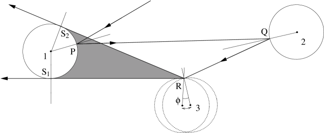
Figure 8: Limitation of the collision angle to $O(a/\ell)$ for recollision events involving multiple scatterers that are separated by distances of $O(\ell)$. Notice that the trajectories between scatterers 1 and 3 are confined within the shaded grey area, which limits the variation of the collision angle at R within a range $\Delta\phi\sim a/\ell$.

In the non-overlapping case the contributions from consecutive collisions with mutually overlapping scatterers need special consideration (in the overlapping case such configurations play no special role). In the diagrammatic representation of the BCE the overlap gives rise to a non-vanishing Mayer-bond between the overlapping scatterers and collision events like the one shown in Fig. 5 correspond to sections of diagrams with two different $T$-operators connected by a Mayer-bond between the two scatterers involved. Either of the two collisions may be real or virtual. The case of two real operators leads to the correction $\delta\lambda_{+}^{\text{(shad)(nov)}}$ of subsection III.2. The case of a real collision followed by a virtual one is responsible for the delay time $t_{d}$ defined in Eq. (34). A virtual collision followed by a real one is responsible for the enhancement $\delta\nu_{\text{c}}^{\text{(lt)}}$ of the collision frequency as specified in Eq. (III.3). The diagram segment with two virtual collisions accounts for the enhancement by $\delta\nu_{\text{c}}^{\text{(lt)}}$ of the damping factor in the survival probability during free flight. Finally, events involving recollisions between overlapping scatterers cancel exactly against the same events without the Mayer-bond between the two scatterers included. In subsection III.2 this was accounted for by restricting the contributions from recollision events involving two nearby scatterers to non-overlapping configurations in the non-overlapping model.

Figure 9: Cancellations between real and virtual collision diagrams in binary collision expansion for repeated collisions between the point particle and multiple scatterers separated by distances of $O(\ell)$.

Recollisions where the point particle returns to a scatterer from a distance of the order of the mean free path, restrict the allowed collision angle at the preceding collision to an angular range of the order $a/\ell\sim\tilde{n}$ (see Fig. 8). Therefore, at the level of corrections to $\lambda_{+}$ restricted to order $\tilde{n}^{2}$, no further restrictions may be imposed on the free flight lengths and collision angles of the intermediate collisions and all of these lengths typically are of order $\ell$. Now consider, as an example, contributions to $\delta\lambda_{+}$ resulting from the recollision at S in Fig. 9. According to Eq. (11) these come from the averages of $\ln\displaystyle{\frac{\rho_{-}}{\rho_{+}}}$ at S, in case the recollision is real, or at T, in case it is virtual. In either case, the contribution in which the collision at P is virtual, cancels that where the latter is real, through the order of $\tilde{n}$ considered. The same holds true for the contributions from all later collisions. Collisions before the recollision of course are not influenced by it at all. Hence, we conclude that corrections to $\lambda_{+}$ from recollision events involving distances of the order $\ell$ are absent through order $\tilde{n}^{2}$ and we were justified in ignoring these in subsection III.3.

References

- (1) P. Gaspard and G. Nicolis, Phys. Rev. Lett. 65, 1693 (1990).
- (2) D. J. Evans and G. P. Morriss, Statistical Mechanics of Nonequilibrium Liquids, Academic Press, London, (1990).
- (3) J. R. Dorfman, An Introduction to Chaos in Non-Equilibrium Statistical Mechanics, Cambridge Univ. Press, (1999).
- (4) W. G. Hoover, Computational Statistical Mechanics Elsevier Publ. Co., Amsterdam, (1991).
- (5) Ya. G. Sinai, Russ. Math. Surv. 25, 137 (1970).
- (6) To be precise: this holds under the conditions that there is no ”infinite horizon”, i.e. there are no trajectories of infinte length that never hit a scatterer, and, in the case of overlapping scatterers, that the space between the scatterers is percolating (extends to infinity).
- (7) N. S. Krylov, Works on the Foundations of Statistical Mechanics, Princeton University Press, Princeton, (1979).
- (8) H. van Beijeren, J. R. Dorfman, Phys. Rev. Lett. 74, 4412 (1995).
- (9) H. van Beijeren, J. R. Dorfman, Phys. Rev. Lett. 76, 3238 (1996).
- (10) H. van Beijeren, A. Latz, J. R. Dorfman, Phys. Rev. E 57, 4077 (1998).
- (11) Since we use the full collision frequency in our equations this should perhaps rather be called a Lorentz-Enskog equation. Substituting one indeed recovers the Lorentz Boltzmann equation of vBD_prl_95 .
- (12) H. van Beijeren, A. Latz and J. R. Dorfman, Phys. Rev. E 63 016312 (2001)
- (13) Since we only look at the effect of the deviation of the collision probability from that obtained under the assumption of uncorrelated collisions, the precise choice of the lower bound on the time integration does not influence results through order . We chose 0 for convenience.
- (14) H. V. Kruis, Masters thesis, University of Utrecht, The Netherlands (1997).
- (15) D. Panja, Ph.D. thesis, University of Maryland, College Park, USA (2000).
- (16) D. Panja (unpublished).
- (17) J. M. J. van Leeuwen and A. Weyland, Physica 36, 457 (1967); J. M. J. van Leeuwen and A. Weyland, Physica 39, 35 (1968).
- (18) M. H. Ernst, J. R. Dorfman, W. R. Hoegy and J. M. J. van Leeuwen, Physica 45, 127 (1969).
- (19) H. van Beijeren and M. H. Ernst, J. Stat. Phys. 21, 125 (1979).