Kinetic equation for a dense soliton gas

Abstract

We propose a general method to derive kinetic equations for dense soliton gases in physical systems described by integrable nonlinear wave equations. The kinetic equation describes evolution of the spectral distribution function of solitons due to soliton-soliton collisions. Owing to complete integrability of the soliton equations, only pairwise soliton interactions contribute to the solution and the evolution reduces to a transport of the eigenvalues of the associated spectral problem with the corresponding soliton velocities modified by the collisions. The proposed general procedure of the derivation of the kinetic equation is illustrated by the examples of the Korteweg – de Vries (KdV) and nonlinear Schrödinger (NLS) equations. As a simple physical example we construct an explicit solution for the case of interaction of two cold NLS soliton gases.

The concept of soliton plays a fundamental role in nonlinear physics due to its main property—preservation of its parameters during interactions with other solitons in the case of the physically and mathematically important class of so-called integrable equations. Such a particle-like behavior has led to a huge number of investigations of soliton dynamics in various physical systems (see, e.g. scott ) as well as to thorough study of mathematical properties of integrable (or soliton) equations (see, e.g. newell ) initiated in the pioneering paper ggkm where the famous inverse scattering transform (IST) method has been formulated. In this method, each soliton is parameterized by an eigenvalue $\lambda$ of the linear spectral problem associated with the nonlinear wave equation under consideration. For example, the KdV equation

$$u_{t}+6uu_{x}+u_{xxx}=0$$ (1)

is associated with the linear Schrödinger equation

$$\psi_{xx}+u(x,t)\psi=-\lambda^{2}\psi,$$ (2)

so that evolution of the potential $u(x,t)$ according to (1) does not change the spectrum $\lambda$, and, whence, the properties of solitons do not change either. The IST method gives a full explanation of finite-number solitons dynamics and provides the basis for the description of many nonlinear physics phenomena.

We encounter a different physical situation when we have to deal with a dense lattice of solitons. When the solitons in the lattice are correlated they may form a modulated nonlinear periodic wave. The spectral problem (2) for a general periodic in $x$ “potential” $u(x,t)$ leads to the Bloch band structure of the spectrum $\lambda$. The periodic “soliton lattices” are distinguished by a finite number of gaps in the spectrum (see nov ) and the edges $\lambda_{i}$ of the spectral gaps become convenient parameters in terms of which the major physical characteristics of the wave such as wavelength, frequency, amplitude etc are expressed. In a weakly modulated wave the parameters $\lambda_{i}$ become slow functions of space and time coordinates, and their evolution is governed by the Whitham equations whitham . Methods of derivation and integration of the Whitham equations are now well developed and this theory provides an adequate description of such important phenomenon as formation of dispersive shocks (or undular bores) in various physical systems from water surface to space plasma and Bose-Einstein condensate.

Yet another principally different class of problems arises when solitons form a disordered finite-density ensemble (a soliton gas) rather than well-ordered modulated soliton lattice. The relevant physical conditions can be realized for instance when large number of solitons are generated either by random large-scale initial distributions osb or by a stochastic external forcing (such as irregular topography in the internal water wave dynamics), or when they are injected into a ring resonator mitsch . Here it is necessary to introduce an appropriate kinetic description of the soliton gas. We introduce a distribution function $f(x,t;\lambda)$ as the number of solitons with the spectral parameter $\lambda$ in the interval $(\lambda,\lambda+d\lambda)$ and in the space interval $(x,x+dx)$ at the moment $t$. Now, if the soliton dynamics is governed by an exactly integrable equation we arrive at the problem of describing the isospectral evolution of the distribution function $f(x,t;\lambda)$ with time. Since the spectrum $\lambda$ is preserved, the evolution of $f(x,t;\lambda)$ must be governed by the conservation equation

$$f_{t}+(sf)_{x}=0\,,$$ (3)

which means that the eigenvalues $\lambda$ are transferred along the $x$-axis with some mean velocity $s(x,t;\lambda)$ depending on the distribution function $f$ but there is no exchange of $\lambda$’s between different $\lambda$-intervals. Hence, the problem is reduced to finding the velocity $s$ of a soliton gas as a function of $\lambda$, $x$ and $t$. This problem was posed by Zakharov zakh71 as early as in 1971 and he solved it for the case of rarefied gas of KdV solitons. Only recently it was generalized in Ref. el03 to the case of a dense gas of KdV solitons where it was found that velocity $s(x,t;\lambda)$ is determined from the integral equation

$$s(\lambda)=4\lambda^{2}+\frac{1}{\lambda}\int\limits^{\infty}_{0}\ln\left|\frac{\lambda+\mu}{\lambda-\mu}\right|f(\mu)[s(\lambda)-s(\mu)]d\mu,$$ (4)

so that Eqs. (3) and (4) give a closed self-consistent kinetic description of a soliton gas of an arbitrary density. In the limit of rarefied gas, i.e. for $\int f(\mu)d\mu\ll\lambda_{0},$ where $\lambda_{0}$ is a characteristic value of the spectral parameter, the second term in Eq. (4) becomes a small correction to the speeds $4\lambda^{2}$ of non-interacting solitons, and the substitution of $s(\eta)\cong 4\eta^{2},$ $(\eta=\lambda,\mu)$, reproduces the Zakharov kinetic equation zakh71 .

Although a mathematically rigorous derivation of Eq. (4) given in Ref. el03 (which is based on a certain singular limit of the Whitham equations) is quite technical, the final result is physically very natural and suggestive. Indeed, Eq. (4) implies that only two-soliton collisions have to be taken into account (which agrees with the properties of multi-soliton solutions of the KdV equation); thus in a collision of a $\lambda$-soliton (i.e. with the spectral parameter $\lambda$) with a $\mu$-soliton, the coordinate of the $\lambda$-soliton is shifted by the distance

$$\frac{1}{\lambda}\ln\left|\frac{\lambda+\mu}{\lambda-\mu}\right|\quad\text{for}\quad\lambda>\mu,$$

(and there is a similar expression for $\lambda<\mu$), and number of collisions per second is proportional to the relative mean velocity $[s(\mu)-s(\lambda)]$ of these two types of solitons multiplied by the density of $\mu$-solitons. Then, after integration over the distribution function $f(\mu)$ of $\mu$-solitons, we arrive at equation (4) for the speed of $\lambda$-solitons modified by their collisions with the other $\mu$-solitons. It is supposed that the number of the soliton collisions over large distance is large enough and, hence, the mean velocity $s$ is a well-defined variable. As a matter of fact, the typical $x,t$-scales in the kinetic equation are much larger than in the original equation (1). Thus, one can see that the above simple reasoning provides an independent derivation of Eq. (4) for the KdV equation case and, obviously, it can be directly applied to other integrable equations. In this Letter we use this method to derive the kinetic equation for a finite-density gas of bright NLS solitons and infer some its consequences.

As is known, each soliton solution of the focusing NLS equation

$$iu_{t}+u_{xx}+2|u|^{2}u=0$$ (5)

is characterized by a complex eigenvalue

$$\lambda=\alpha+i\gamma,\quad-\infty<\alpha<\infty,\quad 0<\gamma<\infty,$$ (6)

of the Zakharov-Shabat spectral problem and is given by (see, e.g. nov )

$$u(x,t)=2i\gamma\frac{\exp[-2i\alpha x-4i(\alpha^{2}-\gamma^{2})t-i\phi_{0}]}{\cosh[2\gamma(x+4\alpha t-x_{0})]},$$ (7)

that is $\gamma=\Im(\lambda)$ determines the amplitude of the soliton and $\alpha=\Re(\lambda)$ its velocity $v=-4\alpha$. The multi-soliton solution shows that interaction of solitons reduces to only two-soliton elastic collisions and effects of multi-soliton collisions are absent. In accordance with the above argumentation, we consider a gas of solitons characterized by a continuous distribution function of eigenvalues $\lambda$. In other words, $f(x,t;\alpha,\gamma)d\alpha d\gamma dx$ is the number of eigenvalues in the element $d\alpha d\gamma$ of the complex plane $\lambda$ in the space interval $dx$ much greater than both typical soliton width $\sim 1/\gamma$ and average distance between solitons. This distribution function evolves due to motion of solitons and as a consequence of preservation of the spectrum it satisfies again the continuity equation (3) which means conservation of the density of eigenvalues in a given element of $\lambda$-plane. In this equation $s$ denotes mean velocity of $\lambda$-solitons which should be evaluated with the account of soliton collisions. Without interaction of solitons it would be equal to $s(\alpha,\gamma)=-4\alpha$. However, collisions of $\lambda$-soliton $(\lambda=\alpha+i\gamma)$ with other $\mu$-solitons $(\mu=\xi+i\eta)$ modify it in the following way. Each collision of faster $\lambda$-soliton with slower $\mu$-soliton shifts the $\lambda$-soliton forward to the distance (see, e.g. nov )

$$\frac{1}{2\gamma}\ln\left|\frac{\lambda-\overline{\mu}}{\lambda-\mu}\right|^{2}\quad\mathrm{for}\quad s(\alpha,\gamma)>s(\xi,\eta),$$

and the number of such collisions in the time interval $dt$ is equal to the product of the density $f(\xi,\eta)d\xi d\eta$ and the distance overcame by faster $\lambda$-solitons compared with slower $\mu$-solitons, $[s(\alpha,\gamma)-s(\xi,\eta)]dt$. Thus, such collisions increase a path covered by $\lambda$-soliton compared with $-4\alpha dt$. In a similar way, one can calculate the negative shift due to collisions with faster $\mu$-solitons. The total shift is obtained by integration over $d\xi d\eta$. Equating paths $s(\alpha,\gamma)dt$ and $-4\alpha dt+\mathrm{``total\,\,shift"}$, we obtain an integral equation for the self-consistent definition of the soliton gas velocities,

$$\begin{split}s(\alpha,\gamma)=-4\alpha+\frac{1}{2\gamma}\int_{-\infty}^{\infty}\int_{0}^{\infty}\ln\left|\frac{\lambda-\overline{\mu}}{\lambda-\mu}\right|^{2}f(\xi,\eta)\\ \times[s(\alpha,\gamma)-s(\xi,\eta)]d\xi d\eta.\end{split}$$ (8)

Obviously, this derivation of Eq. (8) is correct as long as the resulting velocity $s(\alpha,\gamma)$ is finite. Under this reservation, equations (3) and (8) provide the basis for a consideration of kinetic behavior of dense gas of NLS solitons.

As a simple application of the kinetic equations, let us consider evolution of two beams of solitons, when the spectral distribution gas consists of two monochromatic (“cold”) parts:

$$\begin{split}f(x,t;\xi,\eta)&=\rho_{1}(x,t)\delta(-\xi-\alpha,\eta-\gamma)\\ &+\rho_{2}(x,t)\delta(\xi-\alpha,\eta-\gamma),\end{split}$$ (9)

where $\rho_{1}(x,t)$ corresponds to fast (or moving to the right in the reference system associated with the group velocity of the carrier wave) solitons ($\lambda_{1}=-\alpha+i\gamma$) and $\rho_{2}(x,t)$ to slow (or moving to the left) solitons ($\lambda_{2}=\alpha+i\gamma$). All solitons have the same amplitudes. Of course, the idealized delta-functional approximation for the distribution function in the kinetic equation means that the exact soliton eigenvalues in the original spectral problem for the NLS equation are distributed for $i$-th component within a narrow vicinity of the dominant value $\lambda=\lambda_{i}$ and are actually different, which precludes formation of bound states. The soliton positions in such a “monochromatic” gas are statistically independent which leads to Poisson distribution for the number of solitons in a unit space interval with the mean density $\rho_{i}$ ekmv . It is also clear that one can neglect interactions between the solitons belonging to the same beam compared with the cross-beam interactions.

Substituting (9) into (3), (8) we obtain a “two-beam” reduction of the kinetic equation,

$$\frac{\partial\rho_{1}}{\partial t}+\frac{\partial(s_{1}\rho_{1})}{\partial x}=0,\quad\frac{\partial\rho_{2}}{\partial t}+\frac{\partial(s_{2}\rho_{2})}{\partial x}=0,$$ (10)

where the velocities of the beams $s_{1}=s(-\alpha,\gamma)$ and $s_{2}=s(\alpha,\gamma)$ are determined from the equations

$$s_{1}=4\alpha+\kappa\rho_{2}\cdot(s_{1}-s_{2}),\ \ s_{2}=-4\alpha+\kappa\rho_{1}\cdot(s_{2}-s_{1}),$$ (11)

and the interaction parameter

$$\kappa=\frac{1}{2\gamma}\ln\left(1+\frac{\gamma^{2}}{\alpha^{2}}\right)$$ (12)

is always positive. Resolving (11) we get expressions for velocities in terms of $\rho_{1,2}(x,t)$:

$$s_{1}=4\alpha\frac{1-\kappa(\rho_{1}-\rho_{2})}{1-\kappa(\rho_{1}+\rho_{2})},\ \ s_{2}=-4\alpha\frac{1+\kappa(\rho_{1}-\rho_{2})}{1-\kappa(\rho_{1}+\rho_{2})}.$$ (13)

According to the formulated above condition of applicability of the kinetic description, the densities must satisfy the inequality

$$\kappa(\rho_{1}+\rho_{2})<1.$$ (14)

Substitution of the inverse expressions for $\rho_{1,2}$,

$$\rho_{1}=\frac{s_{2}+4\alpha}{\kappa(s_{2}-s_{1})}\,,\qquad\rho_{2}=\frac{s_{1}-4\alpha}{\kappa(s_{1}-s_{2})}$$ (15)

into the system (10) reduces it to the form

$$\frac{\partial s_{1}}{\partial t}+s_{2}\frac{\partial s_{1}}{\partial x}=0\,,\qquad\frac{\partial s_{2}}{\partial t}+s_{1}\frac{\partial s_{2}}{\partial x}=0,$$ (16)

which is known as the Riemann invariant form of a Chaplygin gas equations which, besides well-known original application to compressible gas dynamics, has recently found a number of other applications. If solution of the system (16) is known, then the densities $\rho_{1},\rho_{2}$ are determined in terms of $s_{1},s_{2}$ by the formulas (15).

Although the system (16) admits the general solution (see, e.g. fer ), we shall confine ourselves to a physically natural problem of the collision (mixing) of slow and fast soliton gases when two gases are separated at the initial moment so that

$$\rho_{1}(x,0)=\rho_{10}(x),\quad\rho_{2}(x,0)=0\quad\qquad\hbox{for}\ \ x<0\,,$$ (17)

$$\rho_{1}(x,0)=0,\qquad\rho_{2}(x,0)=\rho_{20}(x)\ \quad\hbox{for}\ \ x>0\,$$ (18)

where $\rho_{10}(x)>0$ and $\rho_{20}(x)>0$ are given functions. Corresponding initial data for the equivalent system (16) follow from (13):

$$s_{1}(x,0)=4\alpha,\ \ \ s_{2}(x,0)=-4\alpha\frac{1+\kappa\rho_{10}(x)}{1-\kappa\rho_{10}(x)},$$ (19)

for $x<0$, and

$$s_{1}(x,0)=4\alpha\frac{1+\kappa\rho_{20}(x)}{1-\kappa\rho_{20}(x)},\ \ \ s_{2}(x,0)=-4\alpha,$$ (20)

for $x>0$. To further simplify the problem, we consider the case when both gases are homogeneous, i.e., $\rho_{10}(x)=\rho_{10}$, $\rho_{20}(x)=\rho_{20}$, where $\rho_{10}$ and $\rho_{20}$ are constant. Since in this case neither the initial conditions, nor the evolution equations (16) contain any parameter with dimension of length, the solution must be self-similar and depend on the variable $x/t$ alone. However, as can be easily seen, the system (16) does not possess non-constant similarity solutions. On the other hand, the solution consisting of two constants $s_{1}\,,s_{2}$ cannot satisfy the discontinuous initial conditions (19), (20). As in shock wave theory whitham , this can be remedied by introducing admissible discontinuities in the solution. The discontinuous “weak” solutions are allowed here owing to the presence of the conservation laws (10), (13). As a result, the sought solution has the form of three constant states $\{f_{1},f_{2}\}:\{\rho_{10},0\},\{\rho_{1c},\rho_{2c}\},\{0,\rho_{20}\}$ separated by two jump discontinuities.

We denote the velocities of the discontinuities as $c^{\pm}\,,\quad c^{+}>c^{-}$. Then the solution is:

(i) $x<c^{-}t$:

$$\rho_{1}\equiv\rho_{1}^{-}=\rho_{10}\,,\quad\rho_{2}\equiv\rho_{2}^{-}=0\,,$$ (21)

which implies by (13),

$$s_{1}\equiv s_{1}^{-}=4\alpha\,,\quad s_{2}\equiv s_{2}^{-}=-4\alpha\frac{1+\kappa\rho_{10}}{1-\kappa\rho_{10}}$$ (22)

(ii) $x>c^{+}t$:

$$\rho_{1}\equiv\rho_{1}^{+}=0,\quad\rho_{2}\equiv\rho_{2}^{+}=\rho_{20},$$ (23)

which implies

$$s_{1}\equiv s_{1}^{+}=4\alpha\frac{1+\kappa\rho_{20}}{1-\kappa\rho_{20}}\,,\quad s_{2}\equiv s_{2}^{+}=-4\alpha.$$ (24)

The values $s_{2}^{-}$ and $s_{1}^{+}$ can be viewed as velocities of trial solitons of one component moving through the homogeneous gas of solitons of another component. One can see that there are critical values for the densities $\rho_{10}=\kappa^{-1}$ and $\rho_{20}=\kappa^{-1}$ yielding the infinite speeds for trial solitons. In accordance with the restriction described above, we assume $\kappa\rho_{10}<1$, $\kappa\rho_{20}<1$.

(iii) $c^{-}t<x<c^{+}t$:

Let $\rho_{1}\equiv\rho_{1c},\,\rho_{2}\equiv\rho_{2c}$ in this interaction zone. Then the four unknown values $\rho_{1c},\rho_{2c},c^{+},c^{-}$ are found from the jump conditions consistent with the physical conservation laws (10) (see, for instance, whitham ):

$$\begin{array}[]{l}-c^{-}[\rho_{1c}-\rho_{1}^{-}]+[\rho_{1c}s_{1c}-\rho_{1}^{-}s_{1}^{-}]=0,\\ -c^{-}[\rho_{2c}-\rho_{2}^{-}]+[\rho_{2c}s_{2c}-\rho_{2}^{-}s_{2}^{-}]=0,\end{array}$$ (25)

$$\begin{array}[]{l}-c^{+}[\rho_{1c}-\rho_{1}^{+}]+[\rho_{1c}s_{1c}-\rho_{1}^{+}s_{1}^{+}]=0,\\ -c^{+}[\rho_{2c}-\rho_{2}^{+}]+[\rho_{2c}s_{2c}-\rho_{2}^{+}s_{2}^{+}]=0.\end{array}$$ (26)

Here

$$s_{1c}=4\alpha\frac{1-\kappa(\rho_{1c}-\rho_{2c})}{1-\kappa(\rho_{1c}+\rho_{2c})},\ \ \ s_{2c}=-4\alpha\frac{1+\kappa(\rho_{1c}-\rho_{2c})}{1-\kappa(\rho_{1c}+\rho_{2c})}.$$ (27)

In view of (21), (23) it readily follows from (25) and (26) that $c^{-}=s_{2c}$ and $c^{+}=s_{1c}$. Then $\rho_{1c}$, $\rho_{2c}$ are found from the same equations with the account of (21), (23) as

$$\rho_{1c}=\frac{\rho_{10}(1-\kappa\rho_{20})}{1-\kappa^{2}\rho_{10}\rho_{20}},\quad\rho_{2c}=\frac{\rho_{20}(1-\kappa\rho_{10})}{1-\kappa^{2}\rho_{10}\rho_{20}}.$$ (28)

Correspondingly, substitution of (28) into (27) yields the velocities of expansion of the interaction region

$$c^{-}=s_{2c}=-4\alpha\frac{1+\kappa\rho_{10}}{1-\kappa\rho_{10}}\quad c^{+}=s_{1c}=4\alpha\frac{1+\kappa\rho_{20}}{1-\kappa\rho_{20}},$$ (29)

and this completes the solution. As one should expect, these velocities coincide with velocities $s_{2}^{-}$ and $s_{1}^{+}$ of the trial solitons (see Eqs. (22) and (24)). Thus, we have found boundaries $x=c^{\pm}t$ of the interaction region and densities $\rho_{1c},$ $\rho_{2c}$ of the two components of soliton gas in this region. In particular, the obtained solution in view of (14) implies that the following inequality is satisfied:

$$F(\rho_{1c},\rho_{2c})=\frac{\rho_{1c}+\rho_{2c}}{\rho_{10}+\rho_{20}}=\frac{1-\frac{2\kappa\rho_{10}\rho_{20}}{\rho_{10}+\rho_{02}}}{1-\kappa^{2}\rho_{10}\rho_{20}}<1.$$ (30)

It means that the total density in the interaction (mixing) zone is always less than the sum of densities of individual separated components.

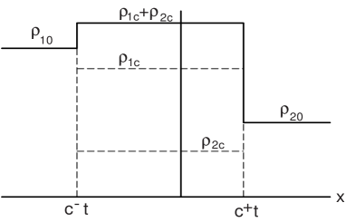
Figure 1: Dependence of solitons densities on space coordinate $x$ at some moment $t$; $\rho_{10}$ and $\rho_{20}$ are the densities of solitons in the beams propagating to the left and to the right, correspondingly; $\rho_{1c}$ and $\rho_{2c}$ are the densities of the same beams in the overlap region.

The process of the collision of two soliton gases is illustrated in Fig. 1. Due to the interaction of solitons with each other, the overlap region spreads out faster than it would without taking into account the phase-shifts caused by two-soliton collisions, and the kinetic equation allows one to give quantitative description of this effect.

In conclusion, we have obtained the kinetic equation describing the evolution of the spectral distribution function of a dense gas of uncorrelated NLS solitons. The proposed procedure of the derivation can be generalized to whole AKNS hierarchy and to other integrable hierarchies. A process of interaction of two “cold” NLS soliton gases is studied in detail.

We are grateful to the Referees for a number of valuable comments. AMK thanks RFBR (grant 05-02-17351) for financial support.

References

- (1) A.C. Scott, Nonlinear Science: Emergence and Dynamics of Coherent Structures, (Oxford University Press, Oxford, 2003).
- (2) A.C. Newell, Solitons in Mathematics and Physics, (SIAM, Philadelphia, 1985).
- (3) C.S. Gardner, J.M. Greene, M.D. Kruskal, and R.M. Miura, Phys. Rev. Lett. 19, 1095 (1967).
- (4) S.P. Novikov, S.V. Manakov, L.P. Pitaevskii, and V.E. Zakharov, Theory of Solitons: The Inverse Scattering Transform, (Plenum, New York, 1984).
- (5) G.B. Whitham, Linear and Nonlinear Waves, (Wiley–Interscience, New York, 1974).
- (6) A.R. Osborne, Phys. Rev. Lett. 71, 3115 (1993).
- (7) F. Mitschke, I. Halama, and A. Schwache, Chaos, Solitons, Fractals, 10, 913 (1999).
- (8) V.E. Zakharov, Zh. Eksp. Teor. Fiz. 60, 993 (1971).
- (9) G.A. El, Phys. Lett. A 311, 374 (2003).
- (10) G.A. El, A.L. Krylov, S.A. Molchanov, and S. Venakides, Physica D 152, 653 (2001).
- (11) E.V. Ferapontov, Phys. Lett. A 158, 112 (1991).