Spatial correlations in SIR epidemic models

Abstract

Abstract: - We investigate the role of global mixing in epidemic processes. We first construct a simplified model of the SIR epidemic using a realistic population distribution. Using this model, we examine possible mechanisms for destruction of spatial correlations, in an attempt to produce correlation curves similar to those reported recently for real epidemiological data. We find that introduction of a long-range interaction destroys spatial correlations very easily if neighbourhood sizes are homogeneous. For inhomogeneous neighbourhoods, very strong long-range coupling is required to achieve a similar effect.

Key-Words: - Epidemic models, lattice gas automata, complex networks

1 Introduction

The main mechanism of transmission of infectious diseases is usually the direct contact of susceptible individuals with an infective one. Since this contact is normally highly localized in space, it is quite natural to expect that space should play an important role in dynamics of infectious diseases. There is a clear evidence that some infectious diseases in animal populations spread geographically. A well-known example is the spatial advance of fox rabies in Europe, which seems to have started in Poland in 1939, and has moved steadily westward at a rate of 30-60 km per year [1]. Similar patterns of spread have been observed in the epizootic of rabies among raccoons in eastern United States and Canada. It started in 1977 in an area on the West Virginia-Virginia border and has moved at a rate of 30-40 km per year [2].

In human populations, the spread of the Black Death in Europe from 1347–1350 is the most often quoted example [3]. Introduced to Italy in 1347, it spread up through Europe at 300-500 km per year. For other diseases the spatial effects appear to be somewhat less pronounced. For example, even though in the past influenza pandemics used to reveal spatial patterns [4], there is a very strong evidence that in recent times the spread of influenza is statistically uniform in space. Bonabeau et al. [5] examined the spatial correlation structure of the influenza epidemic for the epidemic of winter 1994–5, using high-quality data collected by a large network of general practitioners in France. They found that at least for influenza epidemics, space does not play any important role, and the spread of the disease is dominated by the mean-field dynamics.

The goal of this paper is to investigate the role of global mixing in the spread of epidemics. We first construct a simplified model of the SIR epidemic based on realistic population distribution. Using this model, we investigate possible mechanisms for destruction of spatial correlations, trying to achieve similar effects as those reported by Bonabeau et al. [5].

2 Description of the model

In order to study the influence of global mixing on the spread of epidemics we use a model based on interacting particle systems, in the spirit of our earlier work [6, 7]. Models of this type take various forms, ranging from stochastic interacting particle models [8] to models based on cellular automata or coupled map lattices [9, 10, 11, 12].

Consider a set of $N$ individuals, labelled with consecutive integers $1,2\ldots,N$. This set of labels will be denoted by $\mathcal{L}$. We assume that each individual can be in three distinct states, susceptible (S), infected (I) or removed (R). There are two ways to change the state of a single individual. A susceptible individual who comes in direct contact with an infected individual can become infected with probability $p$. Infected individual can become removed with probability $q$. The precise description of the model is as follows.

The state of the $i$-th individual at the time step $k$ will be described by a Boolean vector variable $\boldsymbol{\eta}(i,k)=\langle\eta_{S}(i,k),\eta_{I}(i,k),\eta_{R}(i,k)\rangle$, where $\eta_{\tau}(i,t)=1$ if the $i$-th individual is in the state $\tau$, where $\tau\in\{S,I,R\}$, and $\eta_{\tau}(i,k)=0$ otherwise. We assume that $i=1,2,\ldots,N$ and $k\in\mathbb{N}$, i.e., the time is discrete. Hence, the vector $\boldsymbol{\eta}(i,k)$ can be in one of the following states: $\boldsymbol{\eta}(i,k)=\langle 1,0,0\rangle$ for a susceptible individual, $\boldsymbol{\eta}(i,k)=\langle 0,1,0\rangle$ for an infected individual, and $\boldsymbol{\eta}(i,k)=\langle 0,0,1\rangle$ for a removed individual. No other values of $\boldsymbol{\eta}(i,k)$ are possible in SIR epidemic model. In SIR model an individual can only be at one state at any give time and transitions occur only from susceptible to infected and from infected to removed. The removed does not become susceptible or infected again in SIR model. Therefore, SIR model is suitable for studying spread of influenza in the same season because the same type of influenza virus can infect an individual only once and once the individual is recovered from the flu it becomes immune to this type of virus.

We further assume that at the time step $k$ the $i$-th individual can interact with individuals from a subset of $\mathcal{L}$, to be denoted by $C(i,k)$. Using this notation, we obtain

$$\eta_{S}(i,k+1) = \eta_{S}(i,k)\prod_{j\in C(i,k)}\overline{X_{i,j,k}\eta_{I}(j,k)},$$ (1)

$$\eta_{I}(i,k+1) = \eta_{S}(i,k)\Big{(}1-\prod_{j\in C(i,k)}\overline{X_{i,j,k}\eta_{I}(j,k)}\Big{)}$$ (2)

$$+\eta_{I}(i,k)\overline{Y}_{i},$$

$$\eta_{R}(i,k+1) = \eta_{R}(i,k)+\eta_{I}(i,k)Y_{i},$$ (3)

where $X_{i,j,k}$ is a set of iid Boolean random variables such that $Pr(X_{i,j,k}=1)=p$, $Pr(X_{i,j,k}=0)=1-p$, and $Y_{i}$ is a set of iid Boolean variables such that $Pr(Y_{i}=1)=q$, $Pr(Y_{i}=0)=1-q$.

Note that $X_{i,j,k}=1$ means that the disease has been transmitted from the $j$-th individual to the $i$-th individual at time step $k$. If at least one of the random variables $X_{i,j,k}$ in the product $\prod_{j\in C(i,k)}\overline{X_{i,j,k}\eta_{I}(j,k)}$ takes the value 1, then the product becomes 0, and we obtain $\eta_{S}(i,k+1)=0$, meaning that the $i$-th individual changes its state from susceptible to infected.

The crucial feature of this model is the set $C(i,k)$, representing all individuals with whom the $i$-th individual may have interacted at the time step $k$. In a large human population, it is almost impossible to know $C(i,k)$ for each individual, so we make some simplifying assumptions. First of all, it is clear that the spatial distribution of individuals must be reflected in the structure of $C(i,k)$. We have decided to use realistic population distribution for Southern and Central Ontario using census data obtained from Statistic Canada [13, 14]. The selected region is mostly surrounded by waters of Great Lakes, forming natural boundary conditions. The data set specifies population of so called “dissemination areas” , i.e., small areas composed of one or more neighbouring street blocks. We had access to longitude and latitude data with accuracy of roughly $0.01^{\circ}$, hence some dissemination areas in densely populated regions had the same geographical coordinates. We combined these dissemination areas into larger units, to be called “modified dissemination areas” (MDA).

We will now define the set $C(i,k)$ using the concept of MDAs. This set will be characterized by two positive integers $n_{c}$ and $n_{f}$. Let us label all MDAs in the region we are considering by integers $m=1,2,\ldots,M$, where in our case $M=5069$. For an individual $i$ belonging to the $m$-th MDA, the set $C(i,k)$ consists of all individuals belonging to the $m$-th MDA, plus all individuals belonging to $n_{c}$ MDAs nearest to $m$, plus $n_{f}$ MDAs randomly selected among all remaining MDAs. While the “close neighbours”, i.e., $n_{c}$ nearest MDAs, will not change with time, the “far neighbours”, i.e., $n_{f}$ randomly selected MDAs, will be randomly reselected at each time step.

3 Mean Field

The model described in the previous section involves strong spatial coupling between individuals. Before we describe consequences of this fact, we will first construct a set of equations which approximate dynamics of the model under the assumption of “perfect mixing”, i.e., neglecting the spatial coupling.

The state of the system described by eq. (1–3) at time step $k$ is determined by the states of all individuals and is described by the Boolean random field $\boldsymbol{\eta}(k)=\{\boldsymbol{\eta}(i,k):i=0,\ldots,N\}$. The Boolean field $\{\boldsymbol{\eta}(k):i=0,1,2\ldots\}$ is then a Markov stochastic process.

By taking the expectation $E_{\boldsymbol{\eta}(0)}$ of this Markov process when the initial configuration is $\boldsymbol{\eta}(0)$, i.e. $\rho_{\tau}(i,k)=E_{\boldsymbol{\eta}(0)}\left[\eta_{\tau}(i,k)\right]$ for $\tau\in\{S,I,R\}$, we get the probabilities of the $i$-th individual being susceptible, infected or removed at time $k$.

In the mean field approximation, we assume independence of random variables $\eta_{\tau}(i,k)$. Hence, the expected value of a product of such variables is equal to the product of expected values. Under this assumption, taking expected values of both sides of equations (1–3) we obtain

$$\rho_{S}(i,k+1) = \rho_{S}(i,k)\prod_{j\in C(i,k)}(1-p\rho_{I}(j,k)),$$ (4)

$$\rho_{I}(i,k+1) = \rho_{S}(i,k)\Big{(}1-\prod_{j\in C(i,k)}(1-p\rho_{I}(j,k))\Big{)}$$ (5)

$$+\rho_{I}(i,k)(1-q),$$

$$\rho_{R}(i,k+1) = \rho_{R}(i,k)+\rho_{I}(i,k)q.$$ (6)

Since mean field approximations neglect spatial correlations, we further assume that $\rho_{\tau}(i,k)$ is independent of $i$, i.e., $\rho_{\tau}(i,k)=\rho_{\tau}(k)$. Even though sets $C(i,k)$ have different number of elements for different $i$ and $k$, for the purpose of this approximate derivation we assume that they all have the same number of elements $(1+n_{c}+n_{f})D$, where $D$ is the average MDA population. All these assumptions lead to

$$\rho_{S}(k+1) =\rho_{S}(k)(1-p\rho_{I}(k))^{(1+n_{c}+n_{f})D},$$ (7)

$$\rho_{I}(k+1) =\rho_{I}(k)+\rho_{S}(k)$$

$$-\rho_{S} (k)(1-p\rho_{I}(k))^{(1+n_{c}+n_{f})D}-q\rho_{I}(k),$$ (8)

$$\rho_{R}(k+1) =\rho_{R}(k)+q\rho_{I}(k).$$ (9)

The third equation in the above set is obviously redundant, since $\rho_{S}(k)+\rho_{I}(k)+\rho_{R}(k)=1$.

Similarly to the classical Kermack-McKendrick model, mean field equations (7)-(9) exhibit a threshold phenomenon. Depending on the choice of parameters, we can have $\rho_{I}(k)<\rho_{I}(0)$ for all $k$, meaning that the infection dies out, or we can have an outbreak of the epidemic, meaning that $\rho_{I}(k)>\rho_{I}(0)$ for some $k$. The intermediate scenario of constant $\rho_{I}(k)$ will occur when $\rho_{I}(k)=\rho_{I}(0)$, i.e., when

$$\rho_{S}(0)-\rho_{S}(0)(1-p\rho_{I}(0))^{(1+n_{c}+n_{f})D}-q\rho_{I}(0)=0.$$ (10)

Assuming that initially there are no individuals in the removed group, we have $\rho_{S}(0)=1-\rho_{I}(0)$. Furthermore, if $(1+n_{c}+n_{f})D$ is large, we can assume $(1-p\rho_{I}(0))^{(1+n_{c}+n_{f})D}\approx 1-p(1+n_{c}+n_{f})D\rho_{I}(0)$. Solving eq. (10) for $q$ under these assumptions we obtain

$$q=\Big{(}1-\rho_{I}(0)\Big{)}(1+n_{c}+n_{f})Dp.$$ (11)

Thus, assuming the mean field approximation the epidemic can occur only if $q<\Big{(}1-\rho_{I}(0)\Big{)}(1+n_{c}+n_{f})Dp$.

4 Dynamics of the model

The mean-field equations derived in the previous section depend only on the sum of $n_{c}$ and $n_{f}$. This means, for example, that the model with $n_{c}=5$, $n_{f}=0$ and the model with $n_{c}=0$, $n_{f}=5$ will have the same mean field equations. However, the actual dynamics of these two models will be very different. Depending on the relative size of $n_{f}$ and $n_{c}$, the epidemic may propagate or die out, as we will see in the following analysis.

Let $N_{\tau}(k)$ be the expected value of the total number of individuals belonging to class $\tau\in\{S,I,R\}$,

$$N_{\tau}(k)=E_{\boldsymbol{\eta}(0)}\left(\sum_{i=1}^{N}\eta_{\tau}(i,k))\right).$$

We say that an epidemic occurs if there exists $k>0$ such that $N_{I}(k)>N_{I}(0)$. For fixed $p$, $n_{f}$ and $n_{c}$, there exists a threshold value of $q$ to be denoted by $q_{c}$, such that for each $q<q_{c}$ an epidemic occurs, and for $q>q_{c}$ it does not occur. Obviously $q_{c}$ depends on $p$, and this is illustrated in Figure 1, which shows graphs of $q_{c}$ as a function of $p$ for several different values of $n_{f}$ and $n_{c}$, where $n_{f}+n_{c}=12$. The graphs were obtained numerically by direct computer simulations of the model. The condition $n_{f}+n_{c}=12$ means that the size of the neighbourhood is kept constant, but the proportion of “far neighbours” (represented by $n_{f}$) to “close neighbours” (represented by $n_{c}$) varies.

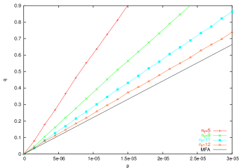
Figure 1: Graphs of critical lines for $n_{f}=5,9,11$, and $12$. In all cases, $n_{c}=12-n_{f}$. Solid line represents mean field approximation.

Figure 1 also shows the mean-field line given by eq. (11).

5 Spatial correlations

As demonstrated in the previous section, the relative size of parameters $n_{f}$ and $n_{c}$ controls dynamics of the epidemic process in a significant way, shifting the critical line up or down. When $n_{c}=0$, i.e., when there are no “far neighbours”, the epidemic process has a strictly local nature, and we can observe well defined epidemic fronts propagating in space. This is illustrated in Figure 2, where the epidemic starts at $k=0$ at a single centrally located MDA (Figure 2a), with $n_{c}=12$, $n_{f}=0$. Modified dissemination areas are represented by pixels colored according to the density of individuals of a given type, such that the red component of the color represents density of infected individuals, green density of susceptibles, and blue density of removed individuals. By density we mean the number of individuals of a given type divided by the population of the MDA.

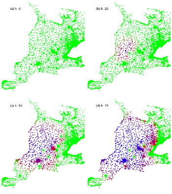
Figure 2: Example of a propagating epidemic front for $n_{c}=12$, $n_{f}=0$, $p=0.00005$, $q=0.05$, with (a) $k=0$, (b) $k=25$, (c) $k=50$ and (d) $k=75$. Modified dissemination areas are represented by pixels colored according to density of individuals of a given type, such that the red component represents density if infected, green density of susceptibles, and blue density of removed individuals.

Epidemic wave propagating outwards can be clearly seen in subsequent snapshots (c), (d) and (e). The front is mostly red, meaning that the bulk of infected individuals is located at the front. After these individuals gradually recover, the center becomes blue.

Let us now consider slightly modified parameters, taking $n_{c}=11$, $n_{f}=1$. This means that we now replace one “close” MDA by one “far” MDA. This does not seem to be a significant change, yet the effect of this change is quite spectacular.

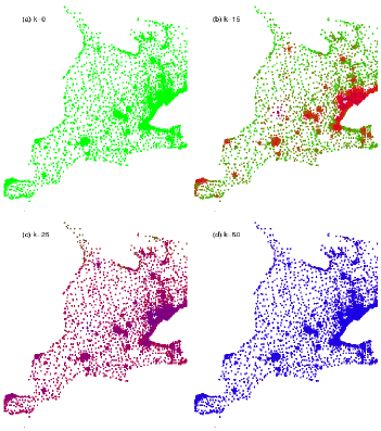
Figure 3: Development of the epidemic for $n_{c}=11$, $n_{f}=1$, $p=0.00005$, $q=0.05$, with (a) $k=0$, (b) $k=15$, (c) $k=25$ and (d) $k=50$. Colour coding is the same as in the previous figure.

As we can see in Figure 3, the epidemic propagates much faster, and there are no visible fronts. The disease quickly spreads over the entire region, and large metropolitan areas become red in a short time, as shown in Figure 3(b). This suggests that infected individuals are more likely to be found in densely populated regions, and their distribution is dictated by the population distribution – unlike in Figure 2, where infected individuals are to be found mainly at the propagating front.

In order to quantify this observation, we use a spatial correlation function for densities of infected individuals defined as

$$h(r,k)=\left\langle\eta_{I}(i,k)\eta_{I}(j,k)\right\rangle_{r\leq d(i,j)\leq r+\Delta r},$$

where $d(i,j)$ is the distance between $i$-th and $j$-th individual, and $<\cdot>$ represents averaging over all pairs $i$, $j$ satisfying condition $r\leq d(i,j)\leq r+\Delta r$. In subsequent considerations we will take $\Delta r=1\,\mathrm{km}$. The distance between two individuals is defined as the distance between MDAs to which they belong.

Consider now a specific example of the epidemic process described by eq. (1-3), where $p=0.000015$, $q=0.2$, and $n_{c}+n_{f}=12$. For this choice of parameters epidemics always occur as long as $n_{f}>0$. Figure 4 shows graphs of the correlation functions $h(r,k_{max})$ at the peak of each epidemic, so that $k_{max}$ is the time step at which the number of infected individuals achieves its maximum value.

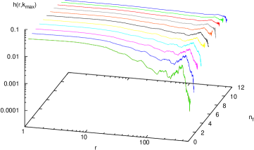
Figure 4: Graphs of the correlation function $h(r,k_{max})$ for different values of $n_{f}$, where $p=0.000015$, $q=0.2$, and $n_{c}+n_{f}=12$.

An interesting phenomenon can be observed in that figure: while the increase of the proportion of “far” neighbours does destroy spatial correlations, one needs very high proportion of “far”neighbours to make the correlation curve completely flat. In [5] it is reported that for influenza epidemics $h(r,k_{max})\sim r^{0.04\pm 0.03}$. If we fit $h(r,k_{max})=Cr^{\alpha}$ curve to the correlation data shown in Figure 4a, we obtain values of the exponent $\alpha$ as shown in Table 1. In order to obtain $\alpha$ of comparably small magnitude as reported in [5], one would have to take $n_{f}$ equal to at least $10$, meaning that $77\%$ of neighbours would have to be “far neighbours”.

$n_{c}$	$n_{f}$	$\alpha$
11	1	-0.72 +/- 0.03
10	2	-0.45 +/- 0.02
9	3	-0.32 +/- 0.01
8	4	-0.27 +/- 0.01
7	5	-0.191 +/- 0.007
6	6	-0.179 +/- 0.009
5	7	-0.120 +/- 0.005
4	8	-0.115 +/- 0.006
3	9	-0.071 +/- 0.003
2	10	-0.057 +/- 0.002
1	11	-0.047 +/- 0.003

Table 1: Values of the exponent $\alpha$ obtained by fitting $h(r,k_{max})=Cr^{\alpha}$ to simulation data.

In reality, this would require that $77\%$ of all individuals one interacted with were not his/her neighbours, coworkers, etc., but individuals from randomly selected and possibly remote geographical regions. This is clearly at odds with our intuition regarding social interactions, especially outside large metropolitan areas. This prompted us to investigate further and to find out what is responsible for this effect.

Upon closer examination of spatial patterns generated in simulations of our model, we reached the conclusion that the inhomogeneity of population sizes in neighbourhoods $C(i,k)$ makes spatial correlations so persistent. Since different MDAs have different population sizes, we expect that some individuals will have larger neighbourhood populations than others, and as a result they will be more likely to get infected, even if the proportion of infected individuals is the same in all MDAs. This will build up clusters of infected individuals around populous MDAs.

To test if this is indeed the factor responsible for strong spatial correlations in our model, we replaced all MDA population sizes with constant population size $D$, i.e., average MDA population size. As expected, graphs of the correlation functions obtained in this case were are all essentially flat, with the exponent $\alpha$ close to zero even in the case of $n_{f}=1$, when we obtained $\alpha=0.023\pm 0.002$.

6 Conclusions

As demonstrated in the previous section, spatial correlations are difficult to destroy if neighbourhood sizes are inhomogeneous. Very strong mixing, i.e., very significant amount of long-range interactions is required to obtain flat correlations curves. On the other hand, for homogeneous neighbourhood sizes, even relatively small long-range interaction immediately forces the process into the perfect-mixing regime, resulting in the lack of spatial correlations.

There is a strong evidence that in recent times epidemics of influenza do not produce significant spatial correlations [5] in spite of the heterogeneity of the population distribution. One can speculate that this must be due to one of the following two factors: either most of our daily interactons are long-ranged, or conversely, most interactions are short-ranged, but the number of interactions per unit time does not vary too greatly from individual to individual.

We suspect that the answer depends on the social and economic structure of the underlying community or adjacent communities. The first scenario applies to large metropolitan areas and conurbations with a large number of commuters, while the second scenario is more likely for small communities without much interaction with the outside word. The above considerations also indicate that a more realistic model will have to separate two aspects of the interaction. First of all, with how many individuals does a given person interact with per unit time, e.g., per day, and how is this number distributed? This could conceivably be determined experimentally without much difficulty. The second aspect is much harder, though: from what pool are these individuals chosen and how? While an accurate answer to this question does not seem to be possible, we hope to get at least some insight from analysis of travel and traffic data. This work is currently in progress and will be presented elsewhere.

Acknowledgement

Henryk Fukś and Anna T. Lawniczak acknowledge partial financial support from the Natural Science and Engineering Research Council (NSERC) of Canada.

References

- [1] Murray J.D. Mathematical Biology II: Spatial Models and Biomedical Applications. Springer Verlag, New York, 2003.
- [2] Centers for Disease Control and Prevention. Update: Raccoon rabies epizootic – United States and Canada. Morbidity and Mortality Weekly Report, vol. 49, 2000, pp. 31–35.
- [3] Langer W.L. Black Death. Scientific American, February 1964, pp. 114–121.
- [4] Rvachev L.A. and Longini I.M. A mathematical model for the global spread of influenza. Math. Biosciences, vol. 75, 1995, pp. 3–22.
- [5] Bonabeau E., Toubiana L., and Flahault A. Evidence for global mixing in real influenza epidemics. J. Phys. A: Math. Gen., vol. 31, 1998, pp. L361–L365.
- [6] Fukś H. and Lawniczak A.T. Individual-based lattice model for the spatial spread of epidemics. Disc. Dyn. in Nat. and Soc., vol. 6, 2001, pp. 191–200. arXiv:nlin.CG/0207048
- [7] Fukś H., Lawniczak A.T., and Di Stefano B. EPILAB: software implementation of epidemic models based on lattice gas cellular automaton. Report FI-NP2000-003, The Fields Institute for Research in Mathematical Sciences, Toronto, 2000.
- [8] Durret R. and Levin S. The importance of being discrete (and spatial). Theoretical Population Biology, vol. 46, 1994, pp. 363–394.
- [9] Schönfisch B. Zelluläre automaten und modelle für epidemien. Ph.D. thesis, Universität Tübingen, 1993.
- [10] Boccara N. and Cheong K. Critical Behaviour of a Probabilistic Automata Network SIS Model for the Spread of an Infectious Disease in a Population of Moving Individuals. J.Phys. A: Math. Gen., vol. 26, 1993, pp. 3707–3717.
- [11] Duryea M., Caraco T., Gardner G., Maniatty W., and Szymanski B.K. Population dispersion and equilibrium infection frequency in a spatial epidemic. Physica D, vol. 132, 1999, pp. 511–519.
- [12] Benyoussef A., Boccara N., Chakib H., and Ez-Zahraouy H. Lattice three-species models of the spatial spread of rabies among foxes. Int. J. Mod. Phys.C vol. 10, 1999, pp. 1025–1038. arXiv:adap-org/9904005
- [13] Statistics Canada. Dissemination Area Digital Cartographic File. Statistics Canada, Geography Division, Ottawa, ON, 2001.
- [14] Statistics Canada. Profile of Age and Sex, for Canada, Provinces, Territories, Census Divisions, Census Subdivisions, and Dissemination Areas, 2001 Census. Industry Canada, Ottawa, ON, 2001.