Independent Component Analysis of Spatiotemporal Chaos

Abstract

Two types of spatiotemporal chaos exhibited by ensembles of coupled nonlinear oscillators are analyzed using independent component analysis (ICA). For diffusively coupled complex Ginzburg-Landau oscillators that exhibit smooth amplitude patterns, ICA extracts localized one-humped basis vectors that reflect the characteristic hole structures of the system, and for nonlocally coupled complex Ginzburg-Landau oscillators with fractal amplitude patterns, ICA extracts localized basis vectors with characteristic gap structures. Statistics of the decomposed signals also provide insight into the complex dynamics of the spatiotemporal chaos.

Spatiotemporal chaos (STC) arising from interaction between autonomous elements is ubiquitous in nonequilibrium dissipative systems such as fluid flows and chemical reactions [1, 2, 3, 4]. It is generally difficult to reduce the complex behavior of strongly coupled systems to the individual dynamics of the component elements, so we must employ collective modes of the system for description. For example, we employ various types of bases in the description of fluids, e.g. Fourier basis, wavelet basis, or eigenfunctions of linearized evolution equations, which represent flow modes such as waves, vortices, and convections [1, 2, 3, 4, 5, 6, 7]. In this case, the observer needs to subjectively choose which basis to use depending on the situation.

On the other hand, there also exist methods of constructing basis functions objectively from statistical properties of the system by some criterion, without explicitly fixing them. A representative method is the principal component analysis (PCA) or the Karhunen-Loéve expansion [5, 6, 7, 8, 9, 10, 11, 12, 13, 14, 15, 16, 17], which is a standard method in multivariate analysis. PCA has already been employed in analyzing STC, for example, to truncate its evolution equation or to estimate its degree of freedom [13, 14, 15, 16, 17]. However, as we show below, when PCA is applied to STC, spatially delocalized bases are typically extracted, which are not appropriate for describing local field structures. Particularly, when the system has translational symmetry, it can be proven that PCA extracts the Fourier basis itself. Therefore, some statistical method that can objectively and compactly capture the complex field structures is desirable.

In this letter, we apply independent component analysis (ICA) to STC. ICA is a recently developed method of statistical signal processing, which attempts to decompose observed mixed signals into maximally independent signals [8, 9, 10, 11, 12]. It is known that the ICA basis gives an information-theoretically efficient representation of multivariate signals [8, 9, 10, 11, 12]. We analyze STC exhibited by two types of coupled nonlinear oscillators, namely, locally (diffusively) coupled complex Ginzburg-Landau oscillators (LCGL) [1, 2, 3, 4], and nonlocally coupled complex Ginzburg-Landau oscillators (NCGL) [18, 19, 20, 21, 22], and assess the utility of ICA in analyzing such STC.

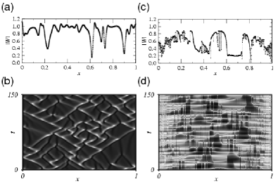
Figure 1: (a) Snapshot and (b) evolution of the amplitude patterns exhibited by LCGL. (c) Snapshot and (d) evolution of the amplitude patterns exhibited by NCGL.

We consider spatially one-dimensional systems of unit length on $[0,1]$. The LCGL is a system of diffusively coupled CGL oscillators, which obeys

$$\frac{\partial W(x,t)}{\partial t}=W-(1+ic_{2})|W|^{2}W+D(1+ic_{1})\frac{\partial^{2}W}{\partial x^{2}},$$ (1)

where $x$ represents the position, $t$ the time, and $W$ the complex amplitude of the CGL oscillator. This is a universal equation derived from general evolution equations for self-oscillatory media by the center-manifold reduction near the supercritical Hopf bifurcation point [1, 2, 3, 4]. Here, $c_{2}$ represents the angular velocity of a single oscillator, $c_{1}$ the phase shift of diffusive coupling, and $D$ the diffusion coefficient. We fix these parameters at $c_{1}=1.0$, $c_{2}=-1.5$, and $D=5\times 10^{-5}$. We assume Neumann boundary conditions $\partial W/\partial x|_{x=0}=\partial W/\partial x|_{x=1}=0$, so that the system is not translationally symmetric. When $c_{1}$ and $c_{2}$ satisfy the Benjamin-Feir condition $1+c_{1}c_{2}<0$, the system exhibits STC. Figure 1(a) shows a typical snapshot of the amplitude pattern $|W(x,t)|$ and Fig. 1(b) its temporal evolution. In this parameter region, the amplitude pattern is composed of characteristic hole structures that move around the system randomly (defect turbulence [1, 2, 3, 4, 23, 24, 25, 26]).

On the other hand, the NCGL is a system of CGL oscillators coupled through a nonlocal mean field weighted by a kernel that decreases exponentially with distance [18, 19, 20, 21, 22]. It obeys

$$\frac{\partial W(x,t)}{\partial t} = W-(1+ic_{2})|W|^{2}W+K(1+ic_{1})$$ (3)

$$\times\left\{\frac{\gamma}{2}\int_{0}^{1}e^{-\gamma|x^{\prime}-x|}W(x^{\prime},t)dx^{\prime}-W\right\},\;\;\;\;\;$$

where $c_{2}$ represents the angular velocity, $c_{1}$ the phase shift of nonlocal coupling, $K$ the coupling strength, and $\gamma^{-1}$ the coupling distance. We fix the parameters at $c_{1}=-2.0$, $c_{2}=2.0$, $\gamma^{-1}=0.125$, and $K=0.85$. We do not assume periodic boundary conditions, and restrict the integration interval to $[0,1]$ (though the kernel is formally normalized in the infinite domain). When the Benjamin-Feir condition $1+c_{1}c_{2}<0$ holds, this system also exhibits STC. However, this STC is considerably different from that of the LCGL. Figure 1(c) shows a typical snapshot of the amplitude pattern $|W(x,t)|$ and Fig. 1(d) its temporal evolution. The amplitude pattern is not continuous but consists of relatively coherent regions and disordered regions with discontinuous gaps. Its power spectrum $I(q)$ exhibits a power-law dependence on the wave number $q$ as shown in Fig. 5 [18, 19, 20, 21, 22]. In this parameter region, such a fractal disordered amplitude pattern evolves steadily.

We focus on the amplitude pattern $|W(x,t)|$ of these two systems hereafter. We discretize a certain domain of space into $n$ segments of length $\Delta x$ and define $u_{i}(t)=|W(i\Delta x,t)|$. The amplitude pattern is now represented by an $n$-dimensional vector $\textbf{u}(t)=(u_{1}(t),\cdots,u_{n}(t))^{T}$, and its temporal sequence is observed. We consider the observed signal and its transformations (denoted by lower-case letters, e.g., ${\bf u}(t)$ or ${\bf z}(t)$), to be the realizations of the underlying stochastic variables (denoted by capital letters, e.g., ${\bf U}$ or ${\bf Z}$). In the following, we subtract the mean value $E[{\textbf{U}}]$ from $\textbf{u}(t)$ and regard $\textbf{z}(t)=(z_{1}(t),\cdots,z_{n}(t))^{T}=\textbf{u}(t)-E[{\textbf{U}}]$ as the observed signal. Here, $E[\cdots]$ denotes the expectation, which is substituted by the long-time average of the observed signal in actual numerical calculations. We decompose $\textbf{z}(t)$ using an $n$-dimensional basis $\{\textbf{a}_{j}\}$ ($j=1\cdots n$) as

$$\textbf{z}(t)=\sum^{n}_{j=1}s_{j}(t)\textbf{a}_{j},$$ (4)

where $\textbf{s}(t)=(s_{1}(t),\cdots,s_{n}(t))^{T}$ represents the decomposed signals. If we use the sinusoidal basis here, this gives a Fourier decomposition. In the following, we use PCA and ICA bases.

PCA extracts orthogonal basis vectors $\{\textbf{a}_{j}\}$ on which the stochastic variable Z distributed in the $n$-dimensional space has the maximum projection (principal components) in order of importance. PCA is achieved by choosing the eigenvectors of the covariance matrix $\boldsymbol{\Sigma}$ of Z as the basis [5, 6, 7, 8, 9, 10, 11, 12]. Namely, each $\{\textbf{a}_{j}\}$ satisfies an eigenequation $\boldsymbol{\Sigma}\textbf{a}_{j}=\lambda_{j}\textbf{a}_{j}$, where $\boldsymbol{\Sigma}=E[\textbf{Z}\textbf{Z}^{T}]=\left(E[Z_{i}Z_{j}]\right)$. Since $\boldsymbol{\Sigma}$ is a real symmetric matrix, $\lambda_{j}\geq 0$ for all $j$. Each $\lambda_{j}$ represents the relative ratio of the $j$-th component $\textbf{a}_{j}$ contained in the observed data. The coefficients $s_{i}(t)$ and $s_{j}(t)$ are uncorrelated when $i\neq j$, but generally not independent.

On the other hand, ICA attempts to extract mutually independent signals $\textbf{s}(t)$ from the observed signals $\textbf{z}(t)$, which are assumed to be a linear mixture of $\textbf{s}(t)$ by some unknown constant $n\times n$ matrix A, i.e., $\textbf{z}(t)=\textbf{A}\textbf{s}(t)$. We assume $\textbf{s}(t)$ to be the outcomes of a stochastic variable S, whose components are mutually independent. It is known that [8, 9, 10, 11, 12] if the number of Gaussian-distributed components of S is at most one (which we assume hereafter), a decomposing matrix W exists such that the decomposed signal $\textbf{y}(t)=(y_{1}(t),\cdots,y_{n}(t))^{T}=\textbf{W}\textbf{z}(t)$ coincides with $\textbf{s}(t)$, except for inevitable ambiguities in the scale and order of the components. To find such a decomposing matrix W, we minimize the mutual information $I(\textbf{Y})$ between the probability density function (PDF) $P(\textbf{y})$ of the stochastic variable $\textbf{Y}=(Y_{1},\cdots,Y_{n})^{T}$ and its marginalized PDFs $P_{i}(y_{i})=\int P(\textbf{y})dy_{1}\cdots dy_{i-1}dy_{i+1}\cdots dy_{n}$,

$$I(\textbf{Y})=\int P(\textbf{y})\log\left(\frac{P(\textbf{y})}{P_{1}(y_{1})\cdots P_{n}(y_{n})}\right)d\textbf{y},$$ (5)

so that the decomposed signals become maximally independent. The matrix W that minimizes $I(\textbf{Y})$ can be obtained using Amari’s natural gradient method [8, 9, 10, 11, 12] as

$$\textbf{W}\leftarrow\textbf{W}-\eta\frac{\partial I(\textbf{Y})}{\partial\textbf{W}}\textbf{W}^{T}\textbf{W}=\textbf{W}+\eta\left(\textbf{I}-E[\boldsymbol{\varphi}(\textbf{Y})\textbf{Y}^{T}]\right)\textbf{W},$$ (6)

where $\eta$ is a learning rate, and $\boldsymbol{\varphi}(\textbf{Y})=(\varphi_{1}(Y_{1}),\cdots,\varphi_{n}(Y_{n}))^{T}$ is a nonlinear vector function of Y. By formally differentiating eq. (5), each component of $\boldsymbol{\varphi}(\textbf{Y})$ is calculated as $\varphi_{i}(Y_{i})=-\partial\log P_{i}(Y_{i})/\partial Y_{i}$, which necessitates knowledge of the unknown functions $P_{i}(Y_{i})$. However, it is known that [8, 9, 10, 11, 12] the signals can be decomposed by assuming simple functional forms for $\varphi_{i}(Y_{i})$ instead of using the true PDF of $Y_{i}$, and various algorithms have been devised. In the following, we use the well-known extended infomax algorithm [8, 9, 10, 11, 12] given by

$$\varphi_{i}(Y_{i})=k_{i}\tanh(Y_{i})+Y_{i},$$ (7)

$$k_{i}=\mbox{sign}\left\{E[1-\tanh^{2}(Y_{i})]E[Y_{i}^{2}]-E[\tanh(Y_{i})Y_{i}]\right\},\;\;\;\;\;$$ (8)

where $k_{i}$ takes either $+1$ or $-1$ depending on the sign of the expression inside the curly brackets. From the estimated decomposing matrix W, ICA basis vectors are obtained as $(\textbf{a}_{1},\cdots,\textbf{a}_{n})=\textbf{W}^{-1}$. When $i\neq j$, the coefficients $s_{i}(t)$ and $s_{j}(t)$ are mutually independent, but $\textbf{a}_{i}$ and $\textbf{a}_{j}$ are generally not orthogonal.

In actual numerical calculations, the LCGL and NCGL are numerically simulated using $N=2^{10}-2^{11}$ spatial grid points. We discretize the central part of the system $0.375\leq x<0.625$ using $n=128$ points ($\Delta x=1/512$) and observe the amplitude pattern every second for $20000$ seconds. The decomposing matrix W is initially set to an identity matrix and updated $5000-10000$ times using a learning rate $\eta$ between $0.05-0.3$. Due to the ambiguity of ICA, the extracted vectors depend on the observed data and on the initial condition for W, even if the parameters of the systems are the same. Also, we can generally find only local minima in this type of high-dimensional (here $128^{2}$-dimensional) optimization problem. However, in our numerical calculations, we always obtained qualitatively the same results for various data sets, including those obtained using cyclic boundary conditions.

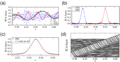
Figure 2: (a) PCA basis vectors No. $1$, $10$, and $100$. (b) ICA basis vectors No. $30$ and $90$. (c) Magnification of ICA basis No. $90$. The dotted line is a fit using the function $1/\cosh[a(x-b)]$, where the parameters are estimated to be $a=141$ and $b=0.551$. (d) All ICA basis vectors. The graph is plotted stereoscopically by gradually shifting the baseline of each basis.

Let us analyze the LCGL first. Figure 2(a) shows three typical basis vectors among $128$ vectors obtained by PCA. These vectors, as well as the other vectors not displayed here, are all roughly sinusoidal and spatially delocalized. Thus, the PCA basis does not capture the local hole structures of the LCGL very well. Figure 2(b) shows two typical basis vectors among $128$ vectors obtained by ICA. Reflecting the characteristic hole structures of the system, spatially localized one-humped vectors are extracted. Each vector can be fitted well by a function given by $1/\cosh[a(x-b)]$, as shown in Fig. 2(c). There is no a priori reason for it to satisfy the LCGL as a special solution [23, 24, 25, 26], but its width is roughly the same as that of the actual hole structures and scales properly with the diffusion constant $D$. All other basis vectors have almost the same shape, but their locations differ from each other, so that the entire observed domain is completely covered, as shown in Fig. 2(d). Here, the obtained basis vectors are sequentially aligned because we used an identity matrix as the initial W. If we use a random matrix as the initial W, we obtain similar basis vectors but their order and vertical orientation become random.

Let us turn our attention to the ICA expansion coefficients (decomposed signals). Since the ICA basis reflects localized hole structures, when the coefficient $s_{j}$ of some basis vector $\textbf{a}_{j}$ takes a large negative value, we can judge that there exists a hole at position $j$. The temporal evolution of a coefficient $s$ corresponding to a typical ICA basis vector (No. $90$) is shown in Fig. 3(a). Corresponding to the appearance of holes, $s$ occasionally takes a large negative value. Figure 3(b) shows PDFs $P(|s|)$ of the absolute value $|s|$ averaged over all signals in logarithmic scales for $s>0$ and $s<0$. Both distributions are super-Gaussian with much heavier tails than the normal distribution. Reflecting the concave asymmetric shape of the vector, $P(|s|)$ for positive $s$ and negative $s$ are different. The tail part of $P(|s|)$ exhibits power-law behavior, implying the existence of some self-similarity in the formation of holes.

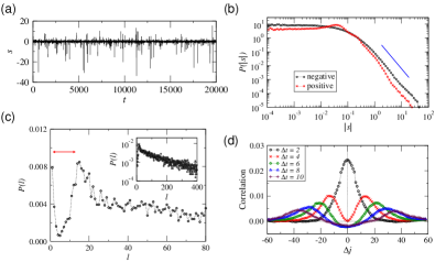
Figure 3: (a) Temporal sequence of the coefficient $s$ of the ICA basis vector No. $90$. (b) PDFs $P(|s|)$ of absolute coefficient $|s|$ for $s>0$ and $s<0$. (c) PDF $P(l)$ of interval $l$ between two successive generation of holes (short time-scale region). The inset shows $P(l)$ at a larger scale. (d) Correlation $C(\Delta j,\Delta t)$ between two decomposed signals.

To characterize the temporal structure of $s$, we investigate the PDF of time interval $l$ between two successive events at which $s$ becomes smaller than some negative threshold $h$. It represents the time interval between two holes, where $h$ determines how large an event must be to be counted as a hole. Figure 3(c) displays the PDF $P(l)$ of $l$ for $h=-3$ averaged over all signals. The PDF dips considerably when $0<l<20$ (shown by an arrow), which indicates the existence of refractory periods. After the disappearance of the first hole, the next hole is less likely to appear at the same position for awhile. The PDF decreases exponentially at large values of $l$ as shown in the inset, indicating a Poissonian random appearance of holes at large time scales.

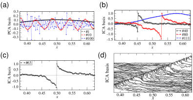
Figure 4: (a) PCA basis vectors No. $1$, $10$, and $100$. (b) ICA basis vectors No. $40$, $80$, and $111$. (c) Magnification of ICA basis vector No. $63$. (d) All ICA basis vectors, drawn stereoscopically by shifting the baselines. A few long-wavelength vectors are omitted.

Figure 3(d) shows correlation functions $C(\Delta j,\Delta t)=\overline{E[s_{j}(t)s_{j+\Delta j}(t+\Delta t)]}$ between two signals $s_{j}$ and $s_{j+\Delta j}$ whose index numbers are separated by $\Delta j$ for several values of the temporal difference $\Delta t$. The curves are averaged over $j$ and $t$, and smoothed by averaging over $5$ neighboring data points on both sides. Since the vectors are spatially aligned sequentially, $\Delta j$ corresponds to a spatial distance between two basis vectors. The correlation gradually spreads from neighboring vectors to distant vectors, which clearly captures the dynamics and decoherence of hole structures. Note that the ICA algorithm used here does not take into account the temporal structure of the signals, hence the decomposed signals can be correlated when $\Delta t\neq 0$.

Let us now analyze the NCGL. Examples of PCA basis vectors are shown in Fig. 4(a). All PCA vectors are delocalized and sinusoidal in this case again. Figures 4(b) and 4(c) show ICA basis vectors. As shown in Fig. 4(c), most vectors typically have a localized structure with a gap and two tails, reflecting the gaps of the amplitude pattern of the NCGL. We also found a few (at most $5$ percent of the total number) long-wavelength delocalized vectors such as No. $111$ shown in Fig. 4(b). In the following analysis, we omit such exceptional vectors. The location of each vector is different, and the entire observed domain is covered, as shown in Fig. 4(d). These ICA basis vectors not only reflect the gap structures of the NCGL but also reflect its singularity. As shown in Fig. 5, the power spectrum of the ICA basis vector exhibits a power law similar to that of the original amplitude pattern. Although the statistics are poor, the power-law behavior can readily be seen for a single basis. The average spectrum over all vectors agrees well with the spectrum of the original amplitude pattern. In these respects, the ICA basis captures the given spatial patterns more faithfully than the PCA basis, which does not possess such properties.

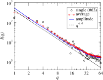
Figure 5: Power spectra of the original amplitude pattern and the ICA basis vectors of the NCGL. Circles($\circ$) represent the spectrum of a single ICA basis vector, crosses($+$) the averaged spectrum over all ICA basis vectors, and the solid line the spectrum directly calculated from the amplitude pattern. The broken line is the power-law function $q^{-1.6}$. Each curve is vertically shifted arbitrarily for comparison.

Since each ICA basis vector has a gap structure, its coefficient quantifies a gap in the amplitude pattern. It was shown in previous studies [18, 19, 20, 21, 22] that the difference in amplitude between two nearby oscillators exhibits noisy on-off intermittency [27, 28]. Thus, the ICA coefficient is also expected to exhibit noisy on-off intermittency. Figure 6(a) shows the temporal evolution of a typical ICA coefficient $s$ (No. $63$). Large gap structures are generated intermittently. The PDF $P(|s|)$ of the absolute coefficient $|s|$ averaged over all signals is shown in Fig. 6(b). In this case, $P(|s|)$ for both $s>0$ and $s<0$ is symmetric, since the shape of each basis vector is statistically symmetric. The PDF is super-Gaussian with a flat region for small $|s|$, a power-law region for medium $|s|$, and a sharp cutoff due to nonlinearity at large $|s|$. This shape is characteristic of the noisy on-off intermittency [18, 19, 20, 21, 22]. Figure 6(c) shows the PDF of the laminar length interval $l$ during which $s$ is smaller than some threshold $h$ (here $h=1.5$). It represents the duration between two successive appearances of gap structures. It is known that the laminar length PDF of noisy on-off intermittency is determined by the first passage time PDF of a Wiener process, which has a power-law region $l^{-3/2}$ and an exponential cutoff [27, 28]. This is confirmed in Fig. 6(c) for the ICA coefficient. Finally, Fig. 6(d) shows the correlation $C(\Delta j,\Delta t)$ between signals for several values of $\Delta t$. The correlation does not spread at all in this case, indicating that the ICA basis vectors persist to be independent of each other for a long duration.

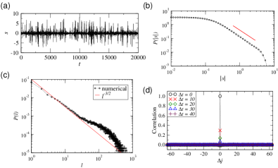
Figure 6: (a) Time sequence of the coefficient $s$ of the ICA basis vector No. $63$. (b) PDFs $P(|s|)$ of the coefficient $|s|$. (c) PDFs $P(l)$ of the laminar length $l$. The straight line is a power-law $l^{-3/2}$. (d) Correlation $C(\Delta j,\Delta t)$ between two decomposed signals.

Summarizing, we applied ICA to STC in two types of coupled oscillators and extracted localized basis vectors that accurately represent the local structures of those systems, which demonstrates the utility of ICA in analyzing the complex spatiotemporal dynamics of nonequilibrium dissipative systems. For the LCGL, ICA extracts a hole structure as a characteristic feature, while for the NCGL, ICA extracts a gap structure with two tails as a characteristic feature. Although there exists no general analytic relationship, the ICA bases obtained in this letter are similar to the wavelet bases [7, 22] in the sense that the basis vectors are localized both in space and in frequency, and cover the entire space by spatial translation. However, these ICA basis vectors do not form a hierarchy over scales through dilatation, which is characteristic of the wavelet basis vectors. The fractality of the amplitude pattern in the NCGL is embodied in the singularity of each basis vector, as shown in Fig. 5. In this letter, we dropped the phase information of the oscillators for simplicity, but the phase also contains important information. In order to capture the phase information, complex ICA of STC, which is conceptually more difficult, is now under investigation.

We thank D. Tanaka, M. Yamada, Y. Iba, H. Suetani and A. Rossberg for useful comments, K. Arai for proofreading the manuscript, and Yukawa Institute of Kyoto University for providing computer facilities.

References

- [1] Y. Kuramoto: Chemical Oscillations, Waves, and Turbulence (Springer, Berlin, 1984).
- [2] P. Manneville: Dissipative Structures and Weak Turbulence (Academic Press, Boston, 1990).
- [3] A. S. Mikhailov and A. Yu. Loskutov: Foundations of Synergetics II (Springer, Berlin, 1996).
- [4] T. Bohr, M. H. Jensen, G. Paladin and A. Vulpiani: Dynamical Systems Approach to Turbulence (Cambridge University Press, Cambridge, 1998).
- [5] J. L. Lumley: Stochastic Tools in Turbulence (Academic Press, New York, 1970).
- [6] L. Sirovich ed.: New Perspectives in Turbulence (Springer, New York, 1990).
- [7] S. Mallat: A Wavelet Tour of Signal Processing (Academic Press, San Diego, 1998).
- [8] T.-W. Lee: Independent Component Analysis: Theory and Applications (Kluwer Academic, Boston, 1998).
- [9] A. Hyvärinen, J. Karhunen and E. Oja: Independent Component Analysis (John Wiley & Sons, New York, 2001).
- [10] A. J. Bell and T. J. Sejnowski, Neural Computation 7 (1995) 1129.
- [11] S. Amari, Neural Computation 10 (1998) 251.
- [12] S. Amari and N. Murata ed.: Independent Component Analysis (Saiensu-sha, Tokyo, Japan, 2002) [in Japanese].
- [13] L. Sirovich and J. D. Rodriguez, Phys. Lett. A 120 (1987) 211.
- [14] J. D. Rodriguez and L. Sirovich, Physica D 43 (1990) 77.
- [15] E. Stone and A. Cutler, Physica D 90 (1996) 209.
- [16] S. M. Zoldi and H. S. Greenside, Phys. Rev. Lett. 78 (1997) 1687.
- [17] S. M. Zoldi, J. Liu, K. M. S. Bejaj, H. S. Greenside, and G. Ahlers, Phys. Rev. E 58 (1998) R6903.
- [18] Y. Kuramoto, Prog. Theor. Phys. 94 (1995) 321.
- [19] Y. Kuramoto and H. Nakao, Phys. Rev. Lett. 76 (1996) 4352.
- [20] H. Nakao, Phys. Rev. E 58 (1998) 1591.
- [21] H. Nakao, Chaos 9 (1999) 902.
- [22] H. Nakao, T. Mishiro and M. Yamada, Int. J. Bif. Chaos 11 (2001) 1483.
- [23] B. I. Shraiman, A. Pumir, W. van Saarloos, P. C. Hohenberg, H. Chaté and M. Holen, Physica D 57 (1992) 241.
- [24] H. Chaté, Nonlinearity 7 (1994) 185.
- [25] M. van Hecke, Phys. Rev. Lett. 80 (1998) 1896.
- [26] J. Burguete, H. Chaté, F. Daviaud and N. Mukolobwiez, Phys. Rev. Lett. 82 (1999) 3252.
- [27] T. Yamada and H. Fujisaka, Prog. Theor. Phys. 76 (1986) 582.
- [28] A. Čenys, A. N. Anagnostopoulos and G. L. Bleris, Phys. Lett. A 224 (1997) 346.