Experimental study of two-dimensional enstrophy cascade

Abstract

We study the direct enstrophy cascade in a two-dimensional flow generated in an electromagnetically driven thin layer of fluid. Due to the presence of bottom friction, the energy spectrum deviates from the classical Kraichnan prediction $k^{-3}$. We find that the correction to the spectral slope depends on the thickness on the layer, in agreement with a theoretical prediction based on the analogy with passive scalar statistics.

1 Introduction

Laboratory studies of two-dimensional turbulence are affected by the interaction with the three-dimensional environment in which they are embedded. This interaction is often frictional and generates an additional linear damping term to the equation of motion. A well known example, which is the object of the present letter, is the flow in a shallow layer of fluid, which is subject to the friction with the bottom of the tank where it is contained [1]. Another example is the motion of a soap film dumped from the interaction with the surrounding air [2]. Linear friction dumping is not restricted to laboratory experiments: an important example is the Ekman friction in geophysical fluid dynamics [3].

As predicted in a remarkable paper by Kraichnan in 1967 [4], when a two-dimensional layer of fluids is forced at intermediate scales, smaller than the domain-size and larger than the viscous dissipative length-scales, two different inertial ranges are observed. This is a consequence of the coupled conservation of energy (mean square velocity) and enstrophy (mean square vorticity) in the inviscid limit, a basic difference with respect to three-dimensional turbulence phenomenology. The energy flows toward the large scales giving rise to an inverse energy cascade characterized by the $k^{-5/3}$ Kolmogorov spectrum. Small scale statistics is governed by a direct enstrophy cascade which is expected to develop a smooth flow with $k^{-3}$ energy spectrum, with a possible logarithmic correction [5].

The presence of a linear friction term affects the direct cascade in a dramatic way: the enstrophy flux across scales is no longer constant and the scaling exponent of the spectrum differs from the Kraichnan prediction $k^{-3}$ by a correction proportional to the friction intensity [6, 7]. The origin of this correction can be understood exploiting the analogy between two-dimensional vorticity field and a scalar field passively advected by a smooth velocity field [8]. For the case of a passive scalar with a finite lifetime it is possible to obtain explicit expressions for the scaling exponents of the power spectrum and structure functions which depend on the intensity of the linear dumping and on the statistics of finite-time Lyapunov exponents [9, 10].

In this letter we experimentally study the statistic of the direct enstrophy cascade in a two-dimensional flow generated in an electromagnetically driven thin layer of fluid. This experimental setup has been successfully used for studying several problems connected to two-dimensional turbulence [1, 11, 12]. Here we show that the friction with the bottom of the tank induces a correction on the spectral slope at large wave-numbers, in good agreement with theoretical predictions [6, 7].

2 Experiment

The experimental apparatus consists of a squared Plexiglas tank whose dimensions are $50\times 50$ cm.

The tank is filled with two layers of fluid, subsequentially injected from the bottom. The upper layer of fresh water is placed over a bottom layer of an electrolyte solution of water and NaCl (density $\sim 1060g/l$). At the end of the filling procedure we obtain a stable stratification with controlled fluids thickness. In all the experiments the fluid thickness $h_{1}$ for the lower fluid has been maintained equal to $0.3cm$ while the thickness of the upper fluid $h_{2}$ varies between $0.3$ and $0.7cm$. The total thickness of the two layers will be denoted by $h$.

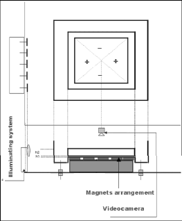
Figure 1: a) A schematic upper view and side view of the experimental setup. b) Snapshot of the velocity field reconstructed by the FT technique on the regular at resolution $128\times 128$ grid for the run $3$ (see Table 1).

Neodymium permanent magnets are placed below the bottom of the tank and disposed in four triangles with magnetic field in the vertical direction and alternating sign (see Fig.1). An electric current, horizontally driven through the cell, interacts with the magnetic field and moves the NaCl solution via the Lorenz force. The forcing current is generated by a computer controlled power supply which provides voltage signal of fixed amplitude and randomly alternating direction. The correlation time for voltage sign reversal is tipically $4s$. The combined action of electric and magnetic forcing on the NaCl solution induces the continuous formation of opposite signed vortical structures whose characteristic length-scale $L_{f}$ is related to the distance between opposite-signed magnets and whose characteristic time-scale is of the order of voltage sign reversal.

The free fluid surface is seeded using tiny buoyant styrene particles (with typical size $d\sim 250\mu m$), and the test section is illuminated using an array of lamps placed orthogonally to one side of the tank. The fluid flow is recorded using a standard speed video camera. A maximum duration of 6 minutes is chosen for each experiment, to ensure that both density stratification and two-dimensionality are maintained [13]. The velocity field has been reconstructed by image analysis based on a Feature Tracking (FT) approach[14]. This tracking procedure allows for higher seeding densities than classical Particle Tracking Velocimetry, and provides an accurate reconstruction of a large number (almost 20000) of Lagrangian trajectories. The interpolated Eulerian velocity field is therefore highly detailed, maximizing the information content of raw data. In Fig. 1 we show an example of instantaneous velocity field reconstructed at resolution $128\times 128$.

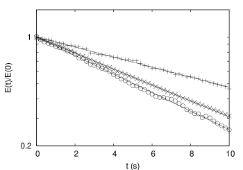
Figure 2: Decay of kinetic energy for the unforced runs (run $1$ $(+)$, run $2$ $(\times)$, run $3$ $(\circ)$). The lines represent exponential fits which give the friction coefficients reported in Table 1.

Table 1: Parameters of the experiments. Friction coefficient $\alpha$, root-mean-square velocity $u_{rms}$, root-mean-square vorticity $\omega_{rms}$, spectral index correction $\xi$

Run #	$h(cm)$	$\alpha(s^{-1})$	$u_{rms}(cms^{-1})$	$\omega_{rms}(s^{-1})$	$\xi$
1	0.8	0.0371	1.324	0.747	0.49
2	0.9	0.0591	1.330	0.640	0.78
3	1.0	0.0686	0.790	0.602	1.02

3 Theory and experimental results

The dynamics of a thin layer of fluid electromagnetically forced is described by the linear dumped 2D Navier-Stokes equations, which can be written for the vorticity $\omega={\bm{\nabla}}\times{\bm{v}}$ as

$${\partial\omega\over\partial t}+{\bm{v}}\cdot{\bm{\nabla}}\omega=\nu\nabla^{2}\omega-\alpha\omega+f(t)$$ (1)

where $\nu$ is the fluid viscosity, $f(t)$ is the time-dependent external forcing. The bottom drag is parameterized by the linear friction term $-\alpha\omega$. Assuming a Poiseuille-like vertical velocity profile, the intensity of the friction coefficient can be related to the total thickness of the layer $h$ as $\alpha\propto\nu/h^{2}$ [15].

Figure 3: Kinetic energy spectrum for the run $1$ ($+$), The dashed line represents the Kraichnan prediction $k^{-3}$. In the inset we show the spectrum compensated with $k^{-3-\xi}$ (solid line) with exponent $\xi$ given in Table 1 and with the Kraichnan prediction $k^{-3}$ (dashed line).

In the inviscid-unforced limit ($\alpha=\nu=f=0$), the NS equations (1) conserves both the kinetic energy $E=1/2\langle v^{2}\rangle$ and the enstrophy $Z=1/2\langle\omega^{2}\rangle$ [16]. For $\alpha>0$ the enstrophy cascading to small scales is removed by friction, allowing to disregard the viscous term in (1)[6]. In this limit, both the energy and the enstrophy decay exponentially in the unforced case with a decaying characteristic time $\tau=1/(2\alpha)$

$$E(t)=E(0)e^{-2\alpha t}\;\;\;\;Z(t)=Z(0)e^{-2\alpha t}$$ (2)

In Figure 2 we plot the decay of the total energy for three experiments with different total thickness $h$ starting from time at which the electric forcing is switched off. The agreement with the exponential decay is remarkable and allow a direct measurement of the friction coefficient $\alpha$. Further this is a confirmation a posteriori of the irrelevance of the viscous term.

The remarkable prediction made in [7] is that for any $\alpha>0$ the Kraichnan scaling exponent in the direct cascade has a correction proportional to $\alpha$. The argument is based on an analogy with the dynamics of a scalar with finite lifetime $\tau=\alpha^{-1}$ passively transported by a smooth flow, which is governed by an equation formally identically to (1) [19]. We remark that the extension of the passive scalar argument [10] to the active vorticity field is not trivial, as $\omega$ determines the velocity field. For completenes, in the following we report the “mean field” derivation of the exponent correction, a complete derivation for the active case can be found in [8].

Figure 4: Kinetic energy spectrum for the run $2$ ($\times$). The dashed line represents the Kraichnan prediction $k^{-3}$. In the inset we show the spectrum compensated with $k^{-3-\xi}$ (solid line) with exponent $\xi$ given in Table 1 and with the Kraichnan prediction $k^{-3}$ (dashed line).

Let us consider a fluctuation of vorticity $\delta\omega(L_{f},0)=\Omega$ generated by the forcing at scale $L_{f}$ and time $0$, i.e. a blob of vorticity of size $L_{f}$ at the rms value $\Omega$. Due to the chaotic flow, the blob is exponentially stretched with a mean rate given by the Lyapunov exponent $\lambda$. Because of the incompressibility of the velocity field, after a time $t$ the blob is contracted in the transverse dimension to a scale $r=L_{f}\exp(-\lambda t)$. This is the mechanism for the direct cascade phenomenon, i.e the fluctuation has been transported from the large injection scale $L_{f}$ to the small scale $r$. Taking into account the decay induced by the friction we can write

$$\delta\omega(r,t)\sim\delta\omega(L_{f},0)e^{-\alpha t}\sim\Omega\left({r\over L_{f}}\right)^{\alpha/\lambda}$$ (3)

In the statistically steady regime sustained by the forcing, this argument provides the scaling exponent for the second-order vorticity structure function:

$$S_{2}(r)\equiv\langle(\delta\omega(r))^{2}\rangle\sim\Omega^{2}\left({r\over L_{f}}\right)^{2\alpha/\lambda}$$ (4)

and thus the scaling exponent of the enstrophy spectrum $Z(k)\sim k^{-1-2\alpha/\lambda}$. Finally one obtain the mean field prediction for the energy spectrum [7]

$$E(k)\sim k^{-3-\xi}$$ (5)

with correction exponent $\xi=2\alpha/\lambda$. We remark that for $\alpha>0$ the correction gives an energy spectrum steeper that $k^{-3}$ which is a posteriori consistent with the assumption of smooth velocity field.

A more refined version of this “mean-field” argument, which takes into account the fluctuations of the Lyapunov exponents [18], can be made [7, 8]. The result is again a correction which makes the spectrum steeper than the Kraichnan prediction. An extensive numerical study of two-dimensional Navier-Stokes equations with friction has confirmed the above theoretical picture [8].

Figures 3, 4 and 5 shows the energy spectra obtained from Fourier transform of the FT velocity data for three experiments with different total thickness in stationary conditions. The spectra are obtained by averaging over about $50$ realizations of the velocity field. A clear cascade range with power-law scaling is evident in intermediate wave-numbers $0.7cm^{-1}<k<4.0cm^{-1}$. The forcing wavenumber $k_{f}\simeq 0.7cm^{-1}$ corresponds to an injection scale $L_{l}\simeq 9\,cm$, consistent with the size of the array of magnets.

A fit of the energy spectra in the range $1.0cm^{-1}<k<4.0cm^{-1}$ gives the exponent corrections $\xi\simeq 0.49$, $\xi\simeq 0.78$ and $\xi\simeq 1.02$ for the three runs respectively. A direct comparison with the theoretical prediction (5) would require the knowledge of the Lyapunov exponent of the flow. It is possible to give a simple estimation by considering the characteristic time in the direct cascade which is given by $\omega_{rms}^{-1}$. Therefore, we can assume that the Lyapunov exponent of the flow is proportional to $\omega_{rms}$, a quantity which is easily determined from the velocity field. Finally, by considering a couple of different runs we have:

$$\frac{\xi_{2}}{\xi_{1}}=\frac{\alpha_{2}}{\alpha_{1}}\frac{\lambda_{1}}{\lambda_{2}}=\frac{\alpha_{2}}{\alpha_{1}}\frac{\omega_{1}}{\omega_{2}}$$ (6)

Using the values of $\alpha_{i}$ and $\omega_{i}$ from table 1 we obtain the predictions $\xi_{1}/\xi_{3}=0.81$ and $\xi_{2}/\xi_{3}=0.44$ which are close to the direct estimation from the spectra $\xi_{1}/\xi_{3}=0.78$ and $\xi_{1}/\xi_{3}=0.49$.

Figure 5: Kinetic energy spectrum for the run $3$ ($\circ$). The dashed line represents the Kraichnan prediction $k^{-3}$. In the inset we show the spectrum compensated with $k^{-3-\xi}$ (solid line) with exponent $\xi$ given in Table 1 and with the Kraichnan prediction $k^{-3}$ (dashed line).

4 Conclusion

In this letter we have presented an experimental study of the effects of bottom friction on the direct enstrophy cascade observed in thin layer of fluid electromagnetically forced. Direct measurements of the friction coefficient are obtained from the exponential decay of the total energy when the forcing is switched off. In the stationary forced case the energy spectra of the reconstructed velocity fields display a power law behavior, with a slope $k^{-3-\xi}$ which differs from the Kraichnan prediction $k^{-3}$. The correction $\xi$ to the spectral slope is due to the friction exerted by the bottom wall on the fluid and increases with the friction intensity. Its value can be predicted by theoretical arguments, in good agreement with our experimental measurements. Being the correction roughly proportional to the square of the inverse of the total thickness of the fluid, the observed effect is expected to be extremely relevant in the case of thin layers.

- [1] \NameParet J. Tabeling P. \REVIEWPhys. Rev. Lett.7919974162.
- [2] \NameRivera M. Wu X.L. \REVIEWPhys. Rev. Lett.852000976.
- [3] \NameSalmon R. \BookGeophysical Fluid Dynamics \PublOxford University Press, New York \Year1998.
- [4] \NameKraichnan H. \REVIEWPhys. of Fluids1019671417.
- [5] \NameKraichnan H. \REVIEWJ. Fluid Mech.471971525.
- [6] \NameD. Bernard \REVIEWEurophys. Lett.502000333
- [7] \NameNam K., Ott E., Antonsen T.M. Guzdar P.N. \REVIEWPhys. Rev. Lett.8420005134.
- [8] \NameBoffetta G.,Celani A.,Musacchio S. Vergassola M. \REVIEWPhys. Rev. E662002026304.
- [9] \NameChertkov M. \REVIEWPhys. of Fluids1019983017
- [10] \NameNam K., Antonsen T.M.,Guzdar P.N. Ott E. \REVIEWPhys. Rev. Lett.8319993426.
- [11] \NameSommeria J. \REVIEWJ. Fluid Mech.1701986139.
- [12] \NameClercx H.J.H, van Heijst G.J.F. Zoeteweij M.L. \REVIEWPhys. Rev. E6720030066303.
- [13] \NameCardoso O., Marteau D. Tabeling P. \REVIEWPhys. Rev. E491994454.
- [14] \NameEspa S. Cenedese A. \REVIEWJ. Visual.2005(in press).
- [15] \NameSatijn M.P., Cense W.A., Verzicco R., Clercx H.J.H van Heijst G.J.F \REVIEWPhys. of Fluids1320011932.
- [16] \NameKraichnan R.H Montgomery D. \REVIEWRep. Prog. Phys. 431980547.
- [17] \NameOtt E. \BookChaos in Dynamical Systems \PublCambridge University Press, Cambridge \Year1993
- [18] \NameBohr T., Jensen M.H, Paladin G. Vulpiani A. \BookDynamical Systems Approach to Turbulence \PublCambridge University Press, Cambridge \Year1998.
- [19] \NameNeufeld Z., Lopez C., Hernandez-Garcia E. Tel T. \REVIEWPhys. Rev. E.6120003857.