DYNAMICS AND STATICS OF VORTICES ON A PLANE AND A SPHERE — I

A. V. BORISOV
Faculty of Mechanics and Mathematics, Department of Theoretical Mechanics Moscow State University
Vorob’ievy gory, 119899 Moscow, Russia
E-mail: borisov@uni.udm.ru
A. E. PAVLOV
Laboratory of Nonlinear Dynamics and Synergetics, Udmurt State University
Universitetskaya Str. 1, 426034. Izhevsk, Russia
E-mail: pavlov@uni.udm.ru

Abstract

In the present paper a description of a problem of point vortices on a plane and a sphere in the “internal” variables is discussed. The Hamiltonian equations of motion of vortices on a plane are built on the Lie–Poisson algebras, and in the case of vortices on a sphere on the quadratic Jacobi algebras. The last ones are obtained by deformation of the corresponding linear algebras. Some partial solutions of the systems of three and four vortices are considered. Stationary and static vortex configurations are found.

1 Dynamics of point vortices on a plane

Introduction

Let us consider the plane motion in boundless ideal liquid of the $N$ rectilinear filaments with the strengths $\Gamma_{i}$, crossing the plane in the points with coordinates $(x_{i},\,y_{i})$. It was shown by Kirchhoff [1] that the motion equations of such system can be written in the Hamiltonian form:

$$\Gamma_{i}\dot{x}_{i}=\frac{\partial H}{\partial y_{i}}\mbox{, }\Gamma_{i}\dot{y}_{i}=-{\frac{\partial H}{\partial x_{i}}}\mbox{, }1\leqslant i\leqslant n,$$ (1)

with the Hamiltonian

$$H=-\frac{1}{8\pi}\sum_{i,j=1}^{N}{{}^{\prime}}\Gamma_{i}\Gamma_{j}\ln M_{ij},$$ (2)

$$M_{ij}\equiv(x_{i}-x_{j})^{2}+(y_{i}-y_{j})^{2},$$

The Poisson brackets are of the form:

$$\{f,\,g\}=\sum_{i=1}^{N}\frac{1}{\Gamma_{i}}\left(\frac{\partial f}{\partial x_{i}}\frac{\partial g}{\partial y_{i}}-\frac{\partial f}{\partial y_{i}}\frac{\partial g}{\partial x_{i}}\right).$$ (3)

The system of equations (1) has, beside of energy (2), the first integrals due to the invariance of the Hamiltonian with respect to translations and rotations of the coordinate system:

$$Q=\sum_{i=1}^{N}\Gamma_{i}x_{i}\mbox{, }P=\sum_{i=1}^{N}\Gamma_{i}y_{i}\mbox{, }I=\sum_{i=1}^{N}\Gamma_{i}(x_{i}^{2}+y_{i}^{2}).$$ (4)

The set of integrals (4) is not in involution:

$$\{Q,\,P\}=\sum_{i=1}^{N}\Gamma_{i}\mbox{, }\{P,\,I\}=-2Q\mbox{, }\{Q,\,I\}=2P.$$ (5)

Representation in “internal” variables

In this paper another representation of problem is given. Let us choose the squares of mutual distances between the point vortices as new variables. For systems of $N$ vortices the number of mutual distances is equal to $N(N-1)/2$. Then, commuting $M_{ij}$ and $M_{lk}$ in the Poisson structure (3) and using the Heron formulas, we as a result obtain some nonlinear Poisson brackets in the phase space determined by mutual distances. However, if we add new variables, the oriented areas of parallelograms spanned on triples of vortices with numbers $i,\>j,\>k$:

$$\triangle_{ijk}\equiv({\bf r}_{j}-{\bf r}_{i})\wedge({\bf r}_{k}-{\bf r}_{i})\mbox{, }{\bf r}_{l}=(x_{l},\,y_{l}),$$ (6)

then in the phase space of the variables $(M_{ij},\,\triangle_{ijk},\,i,\,j,\,k=1,\,\ldots\,,\,N)$ the Lie–Poisson brackets appear. The dimension of the phase is made up of the number of mutual distances between vortices (the number of binomial combinations from $N$ on $2$) and the number of triangles formed by the triples of vortices (the number of binomial combinations of $N$ things ${\bf r}$ at a time) (see Fig. 1): $C_{N}^{2}+C_{N}^{3}=C_{N+1}^{3}$.

Calculation of the Poisson brackets between these variables using (3) leads to the following relations:

$$\{M_{ij},\,M_{kl}\}=4\left(\frac{1}{\Gamma_{i}}\delta_{ik}-\frac{1}{\Gamma_{j}}\delta_{jk}\right)\triangle_{ijl}+4\left(\frac{1}{\Gamma_{i}}\delta_{il}-\frac{1}{\Gamma_{j}}\delta_{jl}\right)\triangle_{ijk};$$ (7)

$$\begin{split}\{M_{ij},\,\triangle_{klm}\}=\left(\frac{1}{\Gamma_{i}}\delta_{ik}-\frac{1}{\Gamma_{j}}\delta_{jk}\right)(M_{li}-M_{im}+M_{mj}-M_{jl})+\\ +\left(\frac{1}{\Gamma_{i}}\delta_{il}-\frac{1}{\Gamma_{j}}\delta_{jl}\right)(M_{mi}-M_{ik}+M_{kj}-M_{jm})+\\ +\left(\frac{1}{\Gamma_{i}}\delta_{im}-\frac{1}{\Gamma_{j}}\delta_{jm}\right)(M_{ki}-M_{il}+M_{lj}-M_{jk});\end{split}$$ (8)

$$\begin{split}\{\triangle_{ijk},\,\triangle_{lmn}\}&=\frac{\delta_{il}}{\Gamma_{i}}(\triangle_{jkn}-\triangle_{jkm})+\frac{\delta_{im}}{\Gamma_{i}}(\triangle_{jkl}-\triangle_{jkn})+\frac{\delta_{in}}{\Gamma_{i}}(\triangle_{jkm}-\triangle_{jkl})+\\ +&\frac{\delta_{jl}}{\Gamma_{j}}(\triangle_{ikm}-\triangle_{ikn})+\frac{\delta_{jm}}{\Gamma_{j}}(\triangle_{ikn}-\triangle_{ikl})+\frac{\delta_{jn}}{\Gamma_{j}}(\triangle_{ikl}-\triangle_{ikm})+\\ +&\frac{\delta_{kl}}{\Gamma_{k}}(\triangle_{ijn}-\triangle_{ijm})+\frac{\delta_{km}}{\Gamma_{k}}(\triangle_{ijl}-\triangle_{ijn})+\frac{\delta_{kn}}{\Gamma_{k}}(\triangle_{ijm}-\triangle_{ijl}).\end{split}$$ (9)

Thus, in the $C_{N+1}^{3}$-dimensional phase space of the variables $(M,\,\triangle)$ the Lie–Poisson brackets are determined. The structure of this algebra is as follows:

$$\{M,\,M\}\subset\triangle\mbox{, }\{M,\triangle\}\subset M\mbox{, }\{\triangle,\,\triangle\}\subset\triangle.$$

Besides the subalgebra $\triangle$, this algebra contains subalgebras of problems of $(N-1)$, $(N-2),\,\ldots$, 3 vortices.

The Poisson brackets are degenerated. The linear Casimir function

$$\triangle=\sum_{i,\,j=1}^{N}\Gamma_{i}\Gamma_{j}M_{ij}$$ (10)

is due to existence of the integral of angular momentum of vortex system. The linear Casimir functions correspond to the trivial geometric relations between the oriented areas of triangles. Let us write here, as an example, one such relation for a quadrangle $\triangle_{ijk}+\triangle_{ikl}-\triangle_{lij}-\triangle_{ljk}=0$ (see Fig. 1). It is easy to see that the annihilator of the brackets is

$$F_{ijkl}=\triangle_{ijk}+\triangle_{ikl}-\triangle_{lij}-\triangle_{ljk}=0.$$ (11)

The structure (9) has also the additional Casimir functions. They came about from such relations as

$$F_{ijk}=(2\triangle_{ijk})^{2}+M_{ij}^{2}+M_{jk}^{2}+M_{ik}^{2}-2(M_{ij}M_{jk}+M_{ij}M_{ik}+M_{jk}M_{ik})=0$$ (12)

derived from the Heron formula, relating the areas and lengthes of sides of a triangle. In general even in the problem of four vortices the functions (12) are not Casimir functions (they determine Casimir functions of subalgebra of three vortices). The detailed analysis and classification of Poisson brackets algebra (9) we plan to present in the next part of our work (to be published).

If we express $\triangle_{ijk}$ from (12) and substitute in the equations of motion for the squares of mutual distances $M_{ij}$, then we get the equations of Laura [2]. Having solved the equations of motion for the relative positions of vortices, we are able to find, using the quadratures and the initial conditions, the absolute coordinates of their positions on a plane at any time [3].

Partial cases of integrability of three and four vortices on a plane

The problems of three and four vortices are of particular interest. The integrability of the problem of three vortices was indicated already by Poincaré. The problem of four vortices is nonintegrable.

Under reduction of the ten-dimensional algebra, corresponding to the problem of four vortices on the general level of six Casimir functions, the Poisson structure becomes nondegenerate. So, according to the Darboux theorem, there exist local canonical coordinates, in which the equations have the form of a usual Hamiltonian system with two degrees of freedom. For integrability of such system, besides the Hamiltonian, one more first integral is required, which, in general case, does not exist.

Let us consider in detail a subalgebra (7)–(9), corresponding to the case of three vortices. In variables $M$, $\triangle$ it has the form:

$$\begin{split}\{M_{1},\,M_{2}\}=-\frac{4}{\Gamma_{3}}\triangle_{4}\mbox{, }\{M_{3},\,M_{1}\}=-\frac{4}{\Gamma_{2}}\triangle_{4}\mbox{, }\{M_{2},\,M_{3}\}=-\frac{4}{\Gamma_{1}}\triangle_{4},\\ \{M_{1},\,\triangle_{4}\}=\left(\frac{1}{\Gamma_{2}}-\frac{1}{\Gamma_{3}}\right)M_{1}+\left(\frac{1}{\Gamma_{2}}+\frac{1}{\Gamma_{3}}\right)(M_{2}-M_{3}),\\ \{M_{2},\,\triangle_{4}\}=\left(\frac{1}{\Gamma_{3}}-\frac{1}{\Gamma_{1}}\right)M_{2}+\left(\frac{1}{\Gamma_{3}}+\frac{1}{\Gamma_{1}}\right)(M_{3}-M_{1}),\\ \{M_{3},\,\triangle_{4}\}=\left(\frac{1}{\Gamma_{1}}-\frac{1}{\Gamma_{2}}\right)M_{3}+\left(\frac{1}{\Gamma_{1}}+\frac{1}{\Gamma_{2}}\right)(M_{1}-M_{2}).\end{split}$$ (13)

The rank of the algebra (13) is two. It corresponds on two-dimensional symplectic leaf to the system with one degree of freedom. Depending on the ratio of intensities, this algebra is a direct sum $SO(3)\oplus\mathbb{R}$ or $SO(1,\,2)\oplus\mathbb{R}$ (the case $\Gamma_{1}+\Gamma_{2}+\Gamma_{3}=0$ is under consideration). Analysis of this problem will be also given in our next publication.

One can point out at an interesting analogy between the problem of three vortices and the system of Lotka–Volterra, appearing in mathematical biology [4].

The Hamiltonian of three vortices

$$H=-\frac{1}{8\pi}(\Gamma_{2}\Gamma_{3}\ln M_{1}+\Gamma_{1}\Gamma_{3}\ln M_{2}+\Gamma_{1}\Gamma_{2}\ln M_{3})$$ (14)

generates the phase flow:

$$\hookrightarrow\dot{M}_{1}=\{M_{1},\,H\}=\frac{\Gamma_{1}}{2\pi}\left(\frac{1}{M_{2}}-\frac{1}{M_{3}}\right)\triangle_{4},$$ (15)

$$\dot{\triangle}_{4}=\frac{1}{8\pi}\left(\frac{\Gamma_{2}+\Gamma_{3}}{M_{1}}(M_{2}-M_{3})+\frac{\Gamma_{1}+\Gamma_{3}}{M_{2}}(M_{3}-M_{1})+\frac{\Gamma_{1}+\Gamma_{2}}{M_{3}}(M_{1}-M_{2})\right).$$

Expressing $\triangle_{4}$ from (12)

$$\triangle_{4}=\pm\frac{1}{2}\sqrt{-M_{1}^{2}-M_{2}^{2}-M_{3}^{2}+2(M_{1}M_{2}+M_{1}M_{3}+M_{2}M_{3})},$$ (16)

we get the system:

$$\hookrightarrow\dot{M}_{1}=\frac{\Gamma_{1}\triangle_{4}}{2\pi M_{1}M_{2}M_{3}}M_{1}(M_{3}-M_{2}).$$ (17)

If we introduce the regularizing time $\tau$:

$$\frac{d\tau}{dt}=\frac{\triangle_{4}}{2\pi M_{1}M_{2}M_{3}},$$ (18)

then we find that $M_{i}$ satisfy the Lotka–Volterra system:

$$\hookrightarrow\frac{d}{d\tau}M_{1}=\Gamma_{1}M_{1}(M_{3}-M_{2}).$$ (19)

Under transition of the system of vortices to a collinear configuration $(\triangle_{4}=0)$ a change of time flow is possible, so one must choose in (16) the sign plus. Hence, we have demonstrated a piecewise trajectory isomorphism between two dynamical problems: the problem of three vortices and the three-dimensional Lotka–Volterra system, which takes place also in the problem of three vortices on a sphere, as it will be shown in the following section.

Let us note a partial case of integrability of four-vortex problem [5]:

$$\sum_{i=1}^{4}\Gamma_{i}=0\mbox{, }Q=P=0.$$ (20)

In this case, the system has sufficient number of integrals $Q$, $P$, $I$, in involution (see the algebra of integrals (5)). Its corresponding Casimir function is $D$ on zero level: $D=0$ due to the relation between the first integrals [6]:

$$D/2=\left(\sum_{i=1}^{N}\Gamma_{i}\right)I-Q^{2}-P^{2}.$$ (21)

Additional invariant relations which are necessary for integrability in variables $M_{ij}$ one can find from the $N(N-1)$ identities [6]

$$f_{ij}\equiv\frac{1}{2}\sum_{k=1}^{N}\Gamma_{k}(M_{jk}-M_{ik})=P(x_{i}-x_{j})+Q(y_{i}-y_{j}),$$ (22)

being valid under $\sum_{i=1}^{N}\Gamma_{i}=0$.

Let us indicate, for example, a particular solution of the system of four vortices if a central symmetry of the configuration takes place [3]. If $\Gamma_{1}=\Gamma_{3}$, $\Gamma_{2}=\Gamma_{4}$ and vortices form a parallelogram on a complex plane $(-z_{1}=z_{3},\ -z_{2}=z_{4})$, then it preserves itself, i. e. in this case there are two invariant relations:

$$M_{1}=L_{1}\mbox{, }M_{3}=L_{3}.$$ (23)

Having chosen an origin of coordinates, coinciding with the fixed symmetry center we can present the equations of motion in the form:

$$\begin{split}\frac{dM_{1}}{d\tau}=\Gamma_{1}M_{1}L_{2}(M_{3}-M_{2})+\Gamma_{2}M_{1}M_{2}(L_{2}-M_{3}),\\ \frac{dM_{3}}{d\tau}=\Gamma_{1}M_{3}L_{2}(M_{2}-M_{1})+\Gamma_{2}M_{2}M_{3}(M_{1}-L_{2}),\\ \frac{dM_{2}}{d\tau}=2\Gamma_{2}M_{2}L_{2}(M_{1}-M_{3})\mbox{, }\frac{dL_{2}}{d\tau}=2\Gamma_{1}M_{2}L_{2}(M_{3}-M_{1}).\end{split}$$ (24)

Here the notation: $L_{2}\equiv M_{24}$ is used and, similarily to (18), the regularization of time $\tau$:

$$\frac{d\tau}{dt}=\frac{\triangle_{4}}{2\pi M_{1}M_{2}M_{3}L_{2}}$$ (25)

is made. The first pair of equations (24) describes motion of the sides of parallelogram and the second one describes motion of its diagonals.

Equations (24) are Hamiltonian with the Hamiltonian:

$$H=2\Gamma_{1}\Gamma_{2}\ln M_{1}+\Gamma_{1}^{2}\ln M_{2}+2\Gamma_{1}\Gamma_{2}\ln M_{3}+\Gamma_{2}^{2}\ln L_{2}.$$ (26)

The Poisson brackets are quartic by elements of the algebra:

$$\begin{split}\{M_{1},M_{2}\}&=\frac{1}{\Gamma_{1}}M_{1}M_{2}M_{3}L_{2},\\ \{M_{1},M_{3}\}&=\frac{1}{2}\left(\frac{1}{\Gamma_{1}}-\frac{1}{\Gamma_{2}}\right)M_{1}M_{2}M_{3}L_{2},\\ \{M_{2},M_{3}\}&=\frac{1}{\Gamma_{1}}M_{1}M_{2}M_{3}L_{2},\\ \{M_{1},L_{2}\}&=-\frac{1}{\Gamma_{2}}M_{1}M_{2}M_{3}L_{2},\\ \{M_{2},L_{2}\}&=0\mbox{, }\{M_{3},L_{2}\}=\frac{1}{\Gamma_{2}}M_{1}M_{2}M_{3}L_{2}.\end{split}$$ (27)

The Poisson structure can be received from the bracket (13) under the restriction on the mentioned above invariant relations. Now, its rank is two. The geometric Casimir function is obtained from the relation between the squares of sides and the squares of diagonals in the parallelogram:

$$F=2(M_{1}+M_{3})-(M_{2}+L_{2}).$$ (28)

For the real motions $F$ is equal to zero.

The Casimir function (10) (“angular momentum” of the system) takes the form:

$$D=\Gamma_{1}M_{2}+\Gamma_{2}L_{2}.$$ (29)

A reduction of system (24) on Casimir functions (28), (29) reduces it to the one-dimensional integrable Hamiltonian one [6].

One must note that in contrast to the rigid body dynamics the equations of motion in the “internal” variables do not have a standard invariant measure as well as even a measure with the analytical positive density. As a result dynamics of these problems is deeply different.

A reduction of system (24) on Casimir functions (28), (29) reduces it to the one-dimensional integrable Hamiltonian one [6].

One must note that in contrast to the rigid body dynamics the equations of motion in the “internal” variables do not have a standard invariant measure as well as even a measure with the analytical positive density. As a result dynamics of these problems is deeply different.

2 Dynamics of point vortices on a sphere

Introduction

Let us consider a problem related to the previous one, a setting of which also goes back to the last century. In work [8] I. S. Gromeka obtained the equations of motion of point vortices on a sphere. The problem presents a simple model, describing a motion of vortex formations (cyclones etc.) in atmosphere of the Earth. The dynamical equations have been written in 1885 year yet were nearly forgot, though the problem in many respects is similar to the problem of motion of point vortices on a plane. In the papers [9, 10] there were pointed to integrability of three vortices on a sphere. In the papers [11, 12] there were proved the integrability of the restricted problem of four vortices.

We shall show that the equations of motion of $N$ vortices on a sphere with the radius $R$ can be presented in the Hamiltonian form with degenerated Poisson structure, assigned by Jacobi algebra $JQ(C^{3}_{N+1})$ [13].

In fact, in the usual canonical basis the equations of motion of $N$ vortices on a sphere can be written in the form:

$$\dot{q}_{k}=\frac{\partial H}{\partial p_{k}}\mbox{, }\dot{p}_{k}=-\frac{\partial H}{\partial q_{k}},$$ (30)

where the canonical coordinates $q_{k}$, $p_{k}$ are expressed through the spherical angles $\theta_{k}$, $\varphi_{k}$ and the strengths $\Gamma_{k}$ as

$$q_{k}=R\sqrt{\Gamma_{k}}\varphi_{k}\mbox{, }p_{k}=R\sqrt{\Gamma_{k}}\cos\theta_{k}.$$ (31)

The Hamiltonian function has the form:

$$H=-\frac{1}{8\pi}\sum_{i,k=1}^{N}{{}^{\prime}}\Gamma_{i}\Gamma_{k}\ln(4R^{2}\sin^{2}\gamma_{ik}/2),$$ (32)

where

$$\cos\gamma_{ik}=\cos\theta_{i}\cos\theta_{k}+\sin\theta_{i}\sin\theta_{k}\cos(\varphi_{i}-\varphi_{k})$$ (33)

is a cosine of the angle between $i$-th and $k$-th radius vectors, connecting the center of sphere with the point vortices (see Fig. 2).

The equations of motion of $N$ point vortices in the spherical system of reference have the following form [9]:

$$\dot{\theta}_{k}=-\frac{1}{4\pi R^{2}}\sum_{i=1}^{N}{{}^{\prime}}\Gamma_{i}\frac{\sin\theta_{i}\sin(\varphi_{k}-\varphi_{i})}{1-\cos\gamma_{ik}},$$

$$\sin\theta_{k}\dot{\varphi}_{k}=\frac{1}{4\pi R^{2}}\sum_{i=1}^{N}{{}^{\prime}}\Gamma_{i}\frac{\sin\theta_{k}\cos\theta_{i}-\cos\theta_{k}\sin\theta_{i}\cos(\varphi_{k}-\varphi_{i})}{1-\cos\gamma_{ik}}.$$ (34)

They are Hamiltonian equations with Poisson brackets

$$\{\varphi_{i},\,\cos\theta_{k}\}=\frac{\delta_{ik}}{R^{2}\Gamma_{i}}.$$ (35)

The system (30) always has four integrals of motion

$$H=c_{0},$$

$$F_{1}\equiv\sum_{i}\Gamma_{i}\sin\theta_{i}\cos\varphi_{i}=c_{1}\mbox{, }F_{2}\equiv\sum_{i}\Gamma_{i}\sin\theta_{i}\sin\varphi_{i}=c_{2}\mbox{, }F_{3}\equiv\sum_{i}\Gamma_{i}\cos\theta_{i}=c_{3},$$ (36)

which, however, are not in involution. It is possible to demonstrate that the integrals $F_{1}$, $F_{2}$, $F_{3}$ commute as components of angular momentum:

$$\{F_{i},\,F_{j}\}=\varepsilon_{ijk}F_{k}.$$ (37)

Algebraic representation

Let us introduce the “internal” variables:

$$M_{ij}\equiv 4R^{2}\sin^{2}\gamma_{ij}/2,$$ (38)

being the squares of spans between arcs of corresponding vortices. The Hamiltonian (32) depends only on introduced mutual variables:

$$H=-\frac{1}{8\pi}\sum_{i,\,k=1}^{N}{{}^{\prime}}\Gamma_{i}\Gamma_{k}\ln M_{ik}.$$ (39)

From the relations between the canonical coordinates $q_{i}$, $p_{j}$ (35) it is possible to find commutators between the values $M_{ik}$:

$$\{M_{ij},\,M_{kl}\}=\frac{4}{R}\left(\frac{1}{\Gamma_{i}}\delta_{ik}-\frac{1}{\Gamma_{j}}\delta_{jk}\right)\triangle_{ijl}+\frac{4}{R}\left(\frac{1}{\Gamma_{i}}\delta_{il}-\frac{1}{\Gamma_{j}}\delta_{jl}\right)\triangle_{ijk},$$ (40)

where the following notations are used:

$$\triangle_{ijk}\equiv{\bf r}_{i}\wedge{\bf r}_{j}\wedge{\bf r}_{k}.$$ (41)

Let us note that we use the same notations in both considered problems. Thus, the Poisson brackets between the values $M_{ik}$ are proportional to external form of volume of parallelepiped spanned on the radius vectors of triple of vortices on a sphere.

It is possible to demonstrate that the algebra of variables $M_{ik}$ and $\triangle_{ijk}$ is closed.

$$\begin{split}\{M_{ij},\,\triangle_{klm}\}=R\left(\frac{1}{\Gamma_{i}}\delta_{ik}-\frac{1}{\Gamma_{j}}\delta_{jk}\right)(M_{li}-M_{im}+M_{mj}-M_{jl})+\\ +R\left(\frac{1}{\Gamma_{i}}\delta_{il}-\frac{1}{\Gamma_{j}}\delta_{jl}\right)(M_{mi}-M_{ik}+M_{kj}-M_{jm})+\\ +R\left(\frac{1}{\Gamma_{i}}\delta_{im}-\frac{1}{\Gamma_{j}}\delta_{jm}\right)(M_{ki}-M_{il}+M_{lj}-M_{jk})+\\ +\frac{1}{2R}\left(\frac{1}{\Gamma_{i}}\delta_{ik}-\frac{1}{\Gamma_{j}}\delta_{jk}\right)(M_{jl}M_{im}-M_{mj}M_{il})+\\ +\frac{1}{2R}\left(\frac{1}{\Gamma_{i}}\delta_{il}-\frac{1}{\Gamma_{j}}\delta_{jl}\right)(M_{jm}M_{ik}-M_{jk}M_{im})+\\ +\frac{1}{2R}\left(\frac{1}{\Gamma_{i}}\delta_{im}-\frac{1}{\Gamma_{j}}\delta_{jm}\right)(M_{jk}M_{il}-M_{ik}M_{jl});\end{split}$$ (42)

$$\begin{split}\{\triangle_{ijk},\,\triangle_{lmn}\}=&\frac{\delta_{il}}{\Gamma_{i}}\left(R(\triangle_{jkn}-\triangle_{jkm})+\frac{1}{2R}(M_{in}\triangle_{jkm}-M_{im}\triangle_{jkn})\right)+\\ +&\frac{\delta_{im}}{\Gamma_{i}}\left(R(\triangle_{jkl}-\triangle_{jkn})+\frac{1}{2R}(M_{il}\triangle_{jkn}-M_{in}\triangle_{jkl})\right)+\\ +&\frac{\delta_{in}}{\Gamma_{i}}\left(R(\triangle_{jkm}-\triangle_{jkl})+\frac{1}{2R}(M_{im}\triangle_{jkl}-M_{il}\triangle_{jkm})\right)+\\ +&\frac{\delta_{jl}}{\Gamma_{j}}\left(R(\triangle_{ikm}-\triangle_{ikn})+\frac{1}{2R}(M_{jm}\triangle_{ikn}-M_{jn}\triangle_{ikm})\right)+\\ +&\frac{\delta_{jm}}{\Gamma_{j}}\left(R(\triangle_{ikn}-\triangle_{ikl})+\frac{1}{2R}(M_{jn}\triangle_{ikl}-M_{jl}\triangle_{ikn})\right)+\\ +&\frac{\delta_{jn}}{\Gamma_{j}}\left(R(\triangle_{ikl}-\triangle_{ikm})+\frac{1}{2R}(M_{jl}\triangle_{ikm}-M_{jm}\triangle_{ikl})\right)+\\ +&\frac{\delta_{kl}}{\Gamma_{k}}\left(R(\triangle_{ijn}-\triangle_{ijm})+\frac{1}{2R}(M_{kn}\triangle_{ijm}-M_{km}\triangle_{ijn})\right)+\\ +&\frac{\delta_{km}}{\Gamma_{k}}\left(R(\triangle_{ijl}-\triangle_{ijn})+\frac{1}{2R}(M_{kl}\triangle_{ijn}-M_{kn}\triangle_{ijl})\right)+\\ +&\frac{\delta_{kn}}{\Gamma_{k}}\left(R(\triangle_{ijm}-\triangle_{ijl})+\frac{1}{2R}(M_{km}\triangle_{ijl}-M_{kl}\triangle_{ijm})\right).\end{split}$$ (43)

The quadratic algebra of vortices on a sphere is presented as a deformation of the linear algebra of vortices on a plane using the parameter — the radius of curvature of sphere $R$. The algebra of vortices on a plane (7)–(9) and the corresponding Casimir functions of system on a sphere are obtained in the limit $R\to\infty:$ $\triangle^{v}\bigm{/}R\to\triangle$, $M^{v}\to M$ from the algebra (40)–(43). Here we symbolically marked by a symbol $v$ ihe variables of the problem on the sphere.

The linear Casimir functions of the quadratic algebra analogous to the corresponding functions of the linear algebra (10)–(11). The analog of the relations (12) can be written as follows:

$$\begin{split}F_{ijk}=&2\triangle_{ijk}{}^{2}+R^{2}(M_{ij}^{2}+M_{ik}^{2}+M_{jk}^{2})-\\ -&2R^{2}(M_{ij}M_{jk}+M_{ik}M_{jk}+M_{ij}M_{ik})+M_{ij}M_{jk}M_{ki}=0.\end{split}$$ (44)

Partial cases of integrabilily of three and four vortices on a sphere

In the spherical problem, the analogue of the partial case on the plane is a situation when the integrals of motion (36) have zero values:

$$F_{1}=F_{2}=F_{3}=0.$$ (45)

The case is completely integrable because there are sufficient number of commuting, on zero level, integrals.

It is not difficult to obtain identity, analogous to (21):

$$D/2=\left(R\sum_{i=1}^{N}\Gamma_{i}\right)^{2}-F_{1}^{2}-F_{2}^{2}-F_{3}^{2}.$$ (46)

Consequently, the considered case corresponds to the level of Casimir function:

$$D/2=\left(R\sum_{i=1}^{N}\Gamma_{i}\right)^{2}.$$

In order to find the invariant relations in variables $M_{ij}$ it is possible to use identity, between absolute and mutual coordinates, analogous to (22):

$$f_{ij}=\frac{1}{2}\sum_{k=1}^{N}\Gamma_{k}(M_{jk}-M_{ik})=R(F_{1}(x_{i}-x_{j})+F_{2}(y_{i}-y_{j})+F_{3}(z_{i}-z_{j})).$$ (47)

3 Stationary vortex states

The obtained forms of the dynamical equations on a plane and on a sphere can be successfully used for finding the steady-state configurations, being the partial solutions of the equations of motion.

Requirements of $N(N-1)/2$ mutual distances $\dot{M}_{ij}=0$ being constant are the conditions of stationary state of vortex configurations. They have the same form both for the configurations on a plane and on a sphere in the “internal” variables as its Hamiltonians (2), (39) and commutation relations $\{M_{ij},\,M_{kl}\}$ (7), (39) have the same form:

$$\sum_{l=1}^{N}{{}^{\prime}}\left(\frac{1}{M_{il}}-\frac{1}{M_{jl}}\right)\Gamma_{l}\triangle_{ijl}(M)=0.$$ (48)

The conditions (48) are very suitable for finding symmetric configurations. On the plane there is solution of $N$ vortices of equal strengths $\Gamma$, disposed in vertices of regular polygon, refined into a circle of radius $R_{0}$. The system rotates with angular velocity

$$\Omega=\frac{\Gamma(N-1)}{4\pi R_{0}^{2}}.$$ (49)

The analysis of stability of such configurations in linear approximation was carried out in [15, 16].

For investigation of such configurations J. J. Thomson was awarded with Adams prize in 1883 [15]. These solutions were at the basis of the theory of vortex atoms propagandized by W. Kelvin (before quantum mechanics). Analogous configuration of identical vortices on a sphere is disposed, according to (52), on latitude $\theta=\theta_{0}$, coordinates $\varphi$ are connected by conditions: $\varphi_{k}-\varphi_{i}=(k-i)2\pi\bigm{/}N$ (see Fig. 3). Angular velocity of rotation about the axis $z$ is:

$$\Omega=\frac{\Gamma(N-1)}{4\pi R_{0}^{2}}\cos\theta_{0}.$$ (50)

The angular velocity of the chain of vortices decreases from poles to equator and on the equator the configuration is static.

The next solution of the system (48) are collinear configurations: $N$ identical vortices on a line rotate with some angular velocity around axis perpendicular to the plane. On the sphere of radius $R$ the collinear configuration ( $N$ atoms on the meridian) rotates around the axis $z$ with angular velocity $\Omega$ (see Fig. 4).

Collinear configurations of vortices on a sphere were not discussed in literature before. We can find them using the following conditions: coordinates $\varphi_{i}$ of the point vortices have the equal values or differ on $\pi$. In addition: $\triangle_{ijl}({\bf M})=0$. It is easy to notice that coordinates $\theta_{i}$, $(0\leqslant\theta\leqslant 2\pi)$ are roots of the following system of trigonometric equations:

$$\frac{4\pi R^{2}\Omega}{\Gamma}\sin\theta_{k}=\sum_{i=1}^{N}{{}^{\prime}}\cot\left(\dfrac{\theta_{k}-\theta_{i}}{2}\right)\mbox{, }(1\leqslant k\leqslant N).$$ (51)

The chain of vortices (51) deserves more attention. The roots of the system assigned the collinear configuration $\theta_{i}$ can be found as equilibrium position of the system of $N$ particles on a circle set by the Hamiltonian

$$H=\frac{1}{2}\sum_{k=1}^{N}p_{k}^{2}+\frac{4\pi R^{2}\Omega}{\Gamma}\sum_{k=1}^{N}\cos\theta_{k}+\sum_{i,\,k=1}^{N}{{}^{\prime}}\ln\left|\sin\frac{\theta_{k}-\theta_{i}}{2}\right|.$$ (52)

Evidently, the positions of equilibrium of the chain of particles coincide with roots of the system (51). Such connection in plane case was marked by Calogero [17]. The locations of identical vortices on a line are set by zeros of Hermitean polynomials of $N$-th power. The system (52) under $\Omega=0$ was considered in [18], where statistical properties of levels of energies of one-dimensional classical Coulomb gas are considered. In the paper [19] the results of equilibrium analysis of the system (52) under condition $\Omega=0:$ $\theta_{i}=\theta_{0}+k\pi\bigm{/}N$, $k=1,\,\ldots\,,\,N$ are adduced.

The problem defined by the Hamiltonian (52) is usually nonintegrable.

Acknowledgements

The work is supported partially by the grant of RFBR (grant No. 96–01–00747).

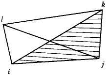
Figure 1:

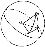
Figure 2:

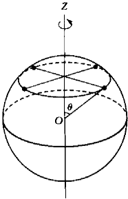
Figure 3:

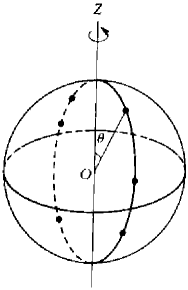
Figure 4:

References

- [1] G. R. Kirchhoff. Vorlesungen über mathematische Physik. 1. Leipzig: Teubner, p. 466.
- [2] E. Laura. Sul moto parallelo ad un plano un fluido in cul vi sono N vortioi elementari // Atti della Reale Accad. Torino, 1902, 37, p. 369-476.
- [3] E. Laura. Sulle equazioni differenziali canoniche del moto di un sistema di vortici elementari, rettilinei e paralleli in un fluido imcompressibile idefinito // Atti della Reale Accad. Torino, 1905, 40, p. 296–312.
- [4] V. Volterra. Leçons sur la theorie mathématique de la lutte pour la vie // Gauthier–Villars, Paris, 1931.
- [5] B. Eckhardt. Integrable four vortex motion // Phys. Fluids., 1988, 31(10), p. 2796–2801.
- [6] V. V. Meleshko, M. Yu. Konstantinov. Dynamics of vortex structures // Kiev: Naukova dumka, 1993, p. 277 (in Russian).
- [7] H. Aref, N. Pomphrey. Integrable and chaotic motions of four vortices I. The case of identical vortices. Proc. R. Soc. Lond., v. 380 A, 1982, p. 359–387.
- [8] I. S. Gromeka. On vortex motions of liquid on a sphere // Collected papers. Moscow, AN USSR, 1952, p. 296 (in Russian).
- [9] V. A. Bogomolov. Two-dimensional fluid dynamics on a sphere // Izv. Acad. Sci. USSR. Atmos. Oceanic Phys., 15, p. 18–22.
- [10] V. A. Bogomolov. Dynamics of vorticity on a sphere // Mech. of liquid and gas. 1977, No. 6, p. 57–65 (in Russian).
- [11] A. A. Bagrets, D. A. Bagrets. Nonintegrability of Hamiltonian systems in vortex dynamics // Reg. & Chaot. Dyn., 1997, 2, No. 1, p. 36–42; 2, No. 2, p. 58–64 (in Russian).
- [12] A. A. Bagrets, D. A. Bagrets. Nonintegrability of two problems in vortex dynamics. Chaos, v. 7, 1997, Issue 3, p. 368–375.
- [13] Ya. L. Granovski, A. S. Zhedanov, I. M. Lutsenko. Quadratic algebras and dynamics in a curved space. II. Kepler’s problem // Teor. i mat. fiz., 1992, 91. No. 3, p. 396–410.
- [14] L. J. Campbell, R. M. Ziff. A catalog of two-dimensional vortex patterns // Los Alamos Sci. Lab. Rep., No. LA–7384–MS. P. 40.
- [15] J. J. Thomson. A treatise on the motion of vortex rings. London: Macmillan, 1883, p. 124.
- [16] L. G. Hazin. Regular polygons of point vortices and resonance instability of stationary states. DAN USSR, v. 230, 1976, No. 4, p. 799-802 (in Russian).
- [17] F. Calogero. Integrable many-body problems. Lectures given at NATO Advanced Study Institute on Nonlinear Equations in Physics and Mathematics, Istanbul, August 1977, p. 3–53.
- [18] F. J. Dyson. Statistical theory of the energy levels of complex systems. I, II, III. J. Math. Phys., v. 3, 1962, No. 1, p. 140–156, p. 157–165, p. 166–175.
- [19] A. M. Perelomov. Integrable systems of classical mechanics and Lie algebras. M.: Nauka. 1990, p. 237.
- [20] D. Hilbert, S. Cohn-Vossen. Anschauliche Geometrie. Berlin, 1932.
- [21] W. Thomson. On the vortex atoms // Phil. Mag. ser. 4, 1867, 34, No. 227, p. 15–24.