Gray soliton solution in the extended nonlinear Schrödinger equation

Abstract

In the framework of extended nonlinear Schrödinger equation (ENSE) the classification of self-similar solutions by the relation between the amplitude and phase is performed. New solutions of ENSE - “gray soliton” and “gray soliton chain” are presented. The properties of these solutions and the possibility for using theirs in physical applications are discussed.

The evolution of the waves in a weakly nonlinear higher order dispersion media can be described by means of the extended nonlinear Schrödinger equation (ENSE)

$$i\frac{\partial\varphi}{\partial t} + \alpha\frac{\partial^{2}\varphi}{\partial y^{2}}+N|\varphi|^{2}\varphi+$$

$$+ i\alpha_{3}\frac{\partial^{3}\varphi}{\partial y^{3}}+i\alpha_{1}|\varphi|^{2}\frac{\partial\varphi}{\partial y}+i\alpha_{2}\varphi\frac{\partial}{\partial y}(|\varphi|^{2})=0.$$

The first three terms in (Gray soliton solution in the extended nonlinear Schrödinger equation) form “classic” nonlinear Schrödinger equation (NSE). The coefficients of equation are connected with properties of propagating waves. So, $\alpha\sim\omega^{\prime\prime}_{kk}$ is the group velocity dispersion ($\omega$ is frequency and $k$ is wave number of carrier wave), $\alpha_{3}$ describes the third-order dispersion, $N$ connects with nonlinear response of the medium. The coefficients $\alpha_{1}$, $\alpha_{2}$ describe the nonlinear dispersion characteristics of medium and their nature depends on the problem under consideration. For example, the appearance of such terms in nonlinear optics is caused on inhomogeneous raman scattering (see, for example Radhakrishnan1996 ), in the nonlinear ferromagnetodynamics the values $\alpha_{1}=\alpha_{2}$ Borich2003 show the dependence of nonlinear response of medium from wave number.

The Eq. (Gray soliton solution in the extended nonlinear Schrödinger equation) is not completely integrable in terms of inverse scattering problem, but there are some integrable cases. The simplest of them $\alpha_{1}=\alpha_{2}=\alpha_{3}=0$, when equation (Gray soliton solution in the extended nonlinear Schrödinger equation) reduce to NSE. The another one is $\alpha_{1}=\alpha_{2}=6\alpha_{3}$, in this case (Gray soliton solution in the extended nonlinear Schrödinger equation) reduces to modified Korteweg - de Vries equation by means of Galileo transformation. For $\alpha_{2}=0$ and $\alpha\alpha_{1}=3\alpha_{3}N$ (Hirota conditions), the ENSE reduces to the Hirota equation Hirota1973 and for $\alpha=1$, $N=2$, $2\alpha_{1}=3\alpha_{3}$, $4\alpha_{1}=3\alpha_{3}$ eq. (Gray soliton solution in the extended nonlinear Schrödinger equation) reduces to the Sasa - Satsuma Sasa1991 equation.

In general case (with arbitrary values of parameters) equation (Gray soliton solution in the extended nonlinear Schrödinger equation) is not completely integrable, but some solutions (and even soliton-like) are known. In our opinion, the most important of them are the follows: “light” and “dark” Potasek - Tabor solitons Potasek1991 , Grudinin1990 , so-called “embedded” and “radiating” solitons Karpman2001 , cnoidal states Smagin2004 and some specific solutions (including “soliton with tail” and “algebraic soliton”) which were found in Gromov1998 (but these solutions realize only for specific values of parameters $\alpha_{1}$, $\alpha_{2}$).

In this paper we try to extend the class of exact solution of ENSE in non integrable case (with arbitrary values of coefficients). We show here that a wide class of solutions can be classified in form of the relation between the nonlinear frequency shift and amplitude of solution.

We suppose solution of (Gray soliton solution in the extended nonlinear Schrödinger equation) in the form of a stationary wave with phase modulation

$$\varphi(y,t)=F(y-vt)\exp\{i(py-qt+\sigma(y-vt))\}.$$ (2)

In this case the equation (Gray soliton solution in the extended nonlinear Schrödinger equation) reduces to the system of two ordinary differential equations (ODEs) for real functions $F(x)$, $\Omega(x)$ (we denote here $x=y-vt$, $\Omega(x)=\sigma^{\prime}_{x}$)

$$(\alpha-3\alpha_{3}(\Omega+p))\frac{d^{2}F}{dx^{2}}-3\alpha_{3}\frac{dF}{dx}\frac{d\Omega}{dx}+$$ (3)

$$+[N-\alpha_{1}(p+\Omega)]F^{3}+$$

$$+[-\alpha(\Omega+p)^{2}+\alpha_{3}(\Omega+p)^{3}-\alpha_{3}\frac{d^{2}\Omega}{dx^{2}}+\Omega v+q]F=0$$

$$\alpha_{3}\frac{d^{3}F}{dx^{3}}+[2\alpha(\Omega+p)-3\alpha_{3}(\Omega+p)^{2}-v]\frac{dF}{dx}+$$ (4)

$$\qquad(\alpha_{1}+2\alpha_{2})F^{2}\frac{dF}{dx}+(\alpha-3\alpha_{3}(p+\Omega))F\frac{d\Omega}{dx}=0.$$

Let us consider the solution of the system of equations (3), (4) in the following form

$$\Omega=A+BF^{n}.$$ (5)

Note, that we do not impose restrictions on possible values of $n$ - it may be any real number, both positive and negative, integer and fractional. Note also, that case $n=1$ was discussed in Gromov1998 and the case $B=0$ was considered in Smagin2004 . By substituting (5) into the system of ODEs (3), (4) and integrating the equation (4) with respect to $x$ we come to the system

$$0 = (\alpha-3\alpha_{3}(A+p))\frac{d^{2}F}{dx^{2}}+[N-\alpha_{1}(A+p)]F^{3}+[-\alpha(A+p)^{2}+\alpha_{3}(A+p)^{3}+vA+q]F-$$

$$- (n+3)\alpha_{3}BF^{n}\frac{d^{2}F}{dx^{2}}-n(n+2)\alpha_{3}BF^{n-1}\Bigg{(}\frac{dF}{dx}\Bigg{)}^{2}+[-2\alpha(A+p)+3\alpha_{3}(A+p)^{2}+v]BF^{1+n}-\alpha_{1}BF^{3+n}+$$

$$+ (-\alpha+3\alpha_{3}(A+p))B^{2}F(x)^{1+2n}+\alpha_{3}B^{3}F(x)^{1+3n},$$

$$0 = \alpha_{3}\frac{d^{2}F}{dx^{2}}+[2\alpha(A+p)-3\alpha_{3}(A+p)^{2}-v]F+\frac{1}{3}(\alpha_{1}+2\alpha_{2})F^{3}+\frac{n+2}{n+1}(\alpha-3\alpha_{3}(A+p))BF^{1+n}-$$

$$- 3\frac{1+n}{1+2n}\alpha_{3}B^{2}F^{1+2n}+C_{1}.$$

Let’s compare the Eq. (Gray soliton solution in the extended nonlinear Schrödinger equation) and Eq. (Gray soliton solution in the extended nonlinear Schrödinger equation). The first of them has two “bad” terms:

$$-(n+3)\alpha_{3}BF^{n}F^{\prime\prime}_{xx},$$ (8)

which is proportional to the product of $n$ power of function $F$ by its second derivation, and

$$-n(n+2)\alpha_{3}BF^{n-1}(F^{\prime}_{x})^{2},$$ (9)

containing the product of $n-1$ power of $F$ and square of its first derivation. We can easy get rid these terms in the following way. At first we multiply the equation (Gray soliton solution in the extended nonlinear Schrödinger equation) by $(n+3)BF^{n}$ and add the result to the (Gray soliton solution in the extended nonlinear Schrödinger equation). Second, we multiply Eq. (Gray soliton solution in the extended nonlinear Schrödinger equation) by $F^{\prime}_{x}$, integrate the result, next find the relation for $(F^{\prime}_{x})^{2}$ from the obtained equation and substitute the result into (Gray soliton solution in the extended nonlinear Schrödinger equation). Thereafter we have the system of two ODEs of the same form:

$$0 = (\alpha-3\alpha_{3}(A+p))\frac{d^{2}F}{dx^{2}}+[-\alpha(A+p)^{2}+\alpha_{3}(A+p)^{3}+vA+q]F+[N-\alpha_{1}(A+p)]F^{3}+2n(n+2)C_{2}BF^{n-1}+$$ (10)

$$+ (n^{2}+3n+2)[2\alpha(A+p)-3\alpha_{3}(A+p)^{2}-v]BF^{1+n}+(3n+5)(\alpha-3\alpha_{3}(A+p))B^{2}F^{1+2n}+$$

$$+ (2n^{2}+5n+3)BC_{1}F^{n}+[(\alpha_{1}+2\alpha_{2})\frac{n^{2}}{6}+(\alpha_{1}+2\alpha_{2})\frac{2n}{3}+2\alpha_{2}]BF^{3+n}-2\frac{3n^{2}+8n+4}{1+2n}\alpha_{3}B^{3}F^{1+3n}$$

$$0 = \alpha_{3}\frac{d^{2}F}{dx^{2}}+[2\alpha(A+p)-3\alpha_{3}(A+p)^{2}-v]F+\frac{1}{3}(\alpha_{1}+2\alpha_{2})F^{3}+\frac{n+2}{n+1}(\alpha-3\alpha_{3}(A+p))BF^{1+n}+$$ (11)

$$- 3\frac{1+n}{1+2n}\alpha_{3}B^{2}F^{1+2n}+C_{1},$$

where $C_{1}$ and $C_{2}$ are constants of integration. The system of this ODEs has nontrivial solutions if the equations (10), (11) coincide, that is they have to contain the value $F(x)$ with same indices of power and proportional coefficients. In this context there are two cases available: (i) all exponents in (10), (11) are different and (ii) some values coincide.

(i). If all exponents have different values, the conditions of compatibility of the system (10), (11) have the follows form:

$$F^{n},F^{0} : C_{1}=0$$ (12)

$$F^{n-1} : C_{2}=0$$

$$F^{3+n} : B\Big{[}\frac{n^{2}}{6}(\alpha_{1}+2\alpha_{2})+\frac{2n}{3}(\alpha_{1}+2\alpha_{2})+2\alpha_{2}\Big{]}=0$$

$$F^{1+3n} : \alpha_{3}B^{2}[3n^{2}+8n+4]=0.$$

We don’t consider here the case $B=0$ - in this case we immediately come to the Duffing equation and brief investigation of available solutions in this situation can be found in Smagin2004 . It is clear from last two equations in (12) that system with $B\neq 0$ may have nontrivial solutions in the only one case:

$$n = -2/3,$$ (13)

$$\alpha_{1} = 17/5\alpha_{2}.$$ (14)

So we have remarkable result: extended NSE has nontrivial solutions only for bounded set of numbers $n$. The equation for $n=-2/3$ has the follow form:

$$0=\alpha_{3}\frac{d^{2}F}{dx^{2}} + \frac{9}{5}\alpha_{2}F^{3}+9(\alpha-3\alpha_{3}p)k_{0}F+$$

$$+ 4(\alpha-3\alpha_{3}p)BF^{1/3}+3\alpha_{3}B^{2}F^{-1/3},$$

with parameters

$$k_{0} = \frac{15\alpha_{3}N-17\alpha\alpha_{2}}{10\alpha_{2}\alpha_{3}},$$ (16)

$$A+p = -\frac{5\alpha_{3}N-9\alpha\alpha_{2}}{10\alpha_{2}\alpha_{3}},$$

$$v = 2\alpha(A+p)-3\alpha_{3}(A+p)^{2}-9(\alpha-3\alpha_{3}p)k_{0},$$

$$q = \alpha(A+p)^{2}-\alpha_{3}(A+p)^{3}-Av+$$

$$+ k_{0}(2\alpha(A+p)-3\alpha_{3}(A+p)^{2}-v).$$

At first sight the existence of physical system with singled out parameters (13), (14) is low - probability.

(ii). Let’s investigate now the case, when there are some coincident values among the indices of power of function $F(x)$ in (10), (11). It appears when $n$ takes on one of the values

$$n = 0,\quad 1,\quad 2,\quad 3,\quad 4,\quad-1,\quad-2,\quad-3,$$

$$\quad-1/2,\quad-1/3,\quad 2/3.$$

For each value from (Gray soliton solution in the extended nonlinear Schrödinger equation) we have its own system of equations and all cases should be analyzed separately. Note, the case $n=0$ is identical to the case $B=0$ (we can rename $A+B\rightarrow A$ in such case). The values $n=-1,-1/2$ are specific because of zeros in denominator. For this values we are to do full transformation chain (3) - (11). As for other values from (Gray soliton solution in the extended nonlinear Schrödinger equation) the final system of ODEs can be found after direct substitution the corresponding value of $n$ into (10) and (11).

After do this we come to the follow conclusion. Nontrivial solutions may be found only in three cases:

1. B = 0. Duffing equation. The classification of possible solutions was performed in Smagin2004 .

2. n = 1. The brief classification of possible states in this situation was published in Gromov1998 .

3. n = -2. This case will be discussed bellow.

The substitution $n=2,3,4,-1,-3,-1/2,-1/3,2/3$ requires the condition $\alpha_{3}=0$. As result we have instead of third-order differential equation a second-order ODE. We are not interesting this situation in our paper.

In the case $n=-2$ we have the equation

$$\frac{d^{2}F}{dx^{2}}+\alpha_{3}^{-1}(2\alpha(A+p)-3\alpha_{3}(A+p)^{2}-v)F +$$ (18)

$$+1/3\alpha_{3}^{-1}(\alpha_{1}+2\alpha_{2})F^{3}-B^{2}F^{-3} = 0$$

whose parameters satisfy the relations

$$C_{1} = 0,$$

$$\frac{\alpha-3\alpha_{3}(A+p)}{\alpha_{3}}=3\frac{N-\alpha_{1}(A+p)}{\alpha_{1}+2\alpha_{2}}=$$

$$= \frac{\frac{2}{3}(\alpha_{2}-\alpha_{1})B-\alpha(A+p)^{2}+\alpha_{3}(A+p)^{3}+vA+q}{2\alpha(A+p)-3\alpha_{3}(A+p)^{2}-v}.$$

The first integral of motion for this equation can be easy calculated

$$\Bigg{(}\frac{dF}{dx}\Bigg{)}^{2} = -\alpha_{3}^{-1}(2\alpha(A+p)-3\alpha_{3}(A+p)^{2}-v)F^{2}-$$ (20)

$$- 1/4\alpha_{3}^{-1}(\alpha_{1}+2\alpha_{2})F^{4}-B^{2}F^{-2}+2E.$$

Let’s consider now the case $(\alpha_{1}+2\alpha_{2})\alpha_{3}<0$. In this situation potential (right - hand part of (20)) is negative for small values of $F$ and increases infinitely for large $F$. So, for small enough $F$ equation (18) have no real solution, whereas for large $F$ the solutions have infinite trajectories. For some values of $E$ potential has three real roots and the finite periodical solutions are possible. This potential for different values of $E$ and corresponded phase portrait is shown in fig. 1.

Figure 1: Phase portrait for the case $(\alpha_{1}+2\alpha_{2})\alpha_{3}<0$

The solutions, corresponded to the finite trajectories in phase portrait on fig. 1 can be defined by means of Jacobi elliptic delta function

$$F(x) = F_{0}\Big{\{}1-\frac{\mu^{2}}{1+\mu^{2}}\mathrm{dn}(bx,k)^{2}\Big{\}}^{1/2}$$ (21)

with parameters

$$F_{0} = \Big{\{}-\frac{2\eta(1+\mu^{2})}{(3+\mu^{2}+k^{2}\mu^{2})\xi}\Big{\}}^{1/2},$$ (22)

$$b = \mu\ \Big{\{}\frac{\eta}{3+\mu^{2}+k^{2}\mu^{2}}\Big{\}}^{1/2},$$

$$E = -\frac{\eta^{2}}{\xi}\frac{\mu^{4}k^{2}+2\mu^{2}+2k^{2}\mu^{2}+3}{(3+\mu^{2}+k^{2}\mu^{2})^{2}},$$

$$B^{2} = \frac{4\eta^{3}}{\xi^{2}}\frac{\mu^{4}k^{2}+\mu^{2}+k^{2}\mu^{2}+1}{(3+\mu^{2}+k^{2}\mu^{2})^{3}},$$

where $\xi$, $\eta$ are coefficients standing before $F^{3}$ and $F$ in (18) respectively. The separatrix solution (potential has the point of contact with F axis, see fig. 1) appears when $k=1$ ($0\leq k\leq 1$ - parameter of elliptic Jacobi function). Returning to the space variable $y$ and to the function $\varphi(y,t)$ and using the relations (22), (Gray soliton solution in the extended nonlinear Schrödinger equation) we find gray soliton solution of extended NSE

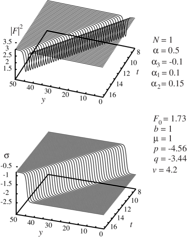
Figure 2: “Gray” soliton in ENSE model

$$\varphi(y,t) = F(y-vt)\exp\{i(py-qt+\sigma(y-vt))\},$$

$$F(y-vt) = F_{0}\Big{\{}1-\frac{\mu^{2}}{1+\mu^{2}}\mathrm{sech}^{2}(b(y-vt))\Big{\}}^{1/2},$$

$$\sigma(y-vt) = \arctan[\mu\tanh(b(y-vt))],$$

$$F_{0}^{2} = -\frac{6\alpha_{3}}{\alpha_{1}+2\alpha_{2}}\frac{1+\mu^{2}}{\mu^{2}}b^{2},$$ (23)

$$p = \frac{\alpha(\alpha_{1}+2\alpha_{2})-3N\alpha_{3}}{6\alpha_{3}\alpha_{2}}+\frac{b}{\mu},$$

$$q = \alpha p^{2}-\alpha_{3}p^{3}-F_{0}^{2}(N-\alpha_{1}p),$$

$$v = 2\alpha p-3\alpha_{3}p^{2}-2\alpha_{3}b^{2}-2(\alpha-3\alpha_{3}p)b/\mu$$

$$- 6\alpha_{3}b^{2}/\mu^{2}.$$

The gray soliton solution of “classic” nonlinear Schrödinger equation was known long ago (see for instance Hasegawa1973 ) but such solution in the ENSE was not known. The evolution of this solution is shown in fig. 2. For numerical simulation we use Fourier transform in $y$-space and fourth-order Runge-Kutta method in $t$- space.

In spite of Potasek - Tabor solitons Potasek1991 this solution has two free parameters (for example thickness $b^{-1}$ and deep of modulation $\mu^{2}/(1+\mu^{2})$, $0<\mu<\infty$). Note also, that amplitude and phase in this solution are connected by means the relation (5). So we can control the deep of modulation by means of nonlinear phase shift, and otherwise we can generate different phase shift using the corresponded deep of modulation. These properties should be fruitful for different physical application.

As for cnoidal solutions (21) at $k\rightarrow 1$ they represent well separated holes on against a background of the carrier wave and can be understand as “1D gray soliton lattice”. Here we discuss the case $(\alpha_{1}+2\alpha_{2})\alpha_{3}<0$. In the opposite case equation (18) also has finite periodical solutions but this situation should be discussed separately.

The authors wish to thank A. Shagalov for fruitful discussions. The work was done within the framework of Program of Basic Researches of the Presidium of RAS “Mathematical method of nonlinear dynamics” and was partially supported by Grant of young scientists and aspirants of Ural Division of RAS No M-06-02-05.

References

• (1) R. Radhakrishnan and M. Lakshmanan, Phys. Rev. E 54, 2949 (1996).
• (2) M. A. Borich, A. V. Kobelev, V. V. Smagin and A. P. Tankeyev, J. Phys.: Cond. Matter 15, 8543 (2003).
• (3) R. Hirota, J. Math. Phys 33 805 (1973).
• (4) N. Sasa and J. Sutsuma, J. Phys. Soc. Japan 60 409 (1991).
• (5) M. J. Potasek and M. Tabor, Phys. Let. 154449 (1991).
• (6) A. B. Grudinin, V. N. Men’shov and T. N. Fursa, Zh. Eksp. Teor. Fiz. 97, 449 (1990).
• (7) V. I. Karpman, J. J. Rasmussen and A. G. Shagalov, Phys. Rev. E 64 026614 (2001).
• (8) V.V. Smagin, M. A. Borich and A. P. Tankeev, The Physics of Metals and Metallography 98, 555 (2004).
• (9) E. M. Gromov and V. V. Tyutin, Wave motion 28 13 (1998).
• (10) A. Hasegawa and F. Tappert, Appl. Phys. Lett. 23, 171 (1973).