“Locally homogeneous turbulence” Is it an inconsistent framework?

Abstract

In his first 1941 paper Kolmogorov assumed that the velocity has increments which are homogeneous and independent of the velocity at a suitable reference point. This assumption of local homogeneity is consistent with the nonlinear dynamics only in an asymptotic sense when the reference point is far away. The inconsistency is illustrated numerically using the Burgers equation. Kolmogorov’s derivation of the four-fifths law for the third-order structure function and its anisotropic generalization are actually valid only for homogeneous turbulence, but a local version due to Duchon and Robert still holds. A Kolomogorov–Landau approach is proposed to handle the effect of fluctuations in the large-scale velocity on small-scale statistical properties; it is is only a mild extension of the 1941 theory and does not incorporate intermittency effects.

The concept of homogeneity, which goes back to Kelvin,kelvin applies to flows whose statistical properties are invariant under (space) translations. For translation-invariant equations, such as the Burgers or Navier–Stokes equations and in the absence of boundaries it is obvious that homogeneity is dynamically preserved. More precisely, with a homogeneous initial velocity field $u_{0}$, as long as the solution is unique, it will also be homogeneous.

A less restrictive condition is that of incremental homogeneity: we now demand only that the statistical properties of the increments $u(x+r)-u(x)$ be invariant under translations, that is depend only on $r$ but not on $x$. In the time domain for which homogeneity is called stationarity, a well-known example of an incrementally stationary random function which is not stationary is the Brownian motion curve. As pointed out by Shiryaev,shiryaev Kolmogorov published in 1940, one year before his famous publications on turbulence, two probability papers. One discusses among other things incremental homogeneity k40a and the other one “Wiener spirals”, self-similar Gaussian random functions now called fractional Brownian motions.k40b He was dealing with random functions whose energy spectrum $E(k)$ has an infrared divergence, that is $\int_{0}^{\infty}E(k)dk$ diverges at $k=0$. For example the Brownian motion has $E(k)\propto k^{-2}$. Turbulence in fluids and plasmas is replete with infrared divergent power-law spectra, for example, the Kolmogorov $k^{-5/3}$ spectrum. In such cases the variance of the velocity increment is finite but the variance of the velocity itself is infinite. Of course, upon introduction of an infrared cutoff $k_{0}>0$, homogeneity is recovered. For example the homogeneous Ornstein–Uhlenbeck Gaussian process which has the spectrum $E(k)=C/(k_{0}^{2}+k^{2})$ goes over into Brownian motion as $k_{0}\to 0$.

In his first 1941 paper k41a (K41) Kolmogorov pointed out the need to work with the increments of the velocity. However, rather than assuming that the turbulence is incrementally homogeneous, he assumed local homogeneity. Specifically he took a space-time reference point $P^{\rm(0)}=({\bm{r}}^{\rm(0)},\,t^{\rm(0)})$ and, for an arbitrary space-time point $P$, considered the space-time increments ${\bm{w}}(P)\equiv{\bm{u}}(P)-{\bm{u}}_{0}$ where ${\bm{u}}_{0}={\bm{u}}(P^{\rm(0)})$ and then defined local homogeneity as the property that for any choice of $n$ points $P_{1}$, $P_{2}$, …, $P_{n}$, the joint distribution of the $n$ increments should be independent of both $P^{\rm(0)}$ and of ${\bm{u}}_{0}$. In other words, Kolmogorov was assuming not only incremental homogeneity and incremental stationarity, he was also assuming independence of the velocity at the reference point.

As stressed by Hill,hill97 ; hill02arxiv various definitions of local homogeneity have been used in the literature. For example Monin and Yaglom my2 mostly take it to be equivalent to incremental homogeneity but, of course, also quote Kolmogorov’s full definition. It is not clear why Kolmogorov felt it necessary to introduce the additional assumption of independence of the velocity at the reference point. It is conceivable that when he wrote his first 1941 turbulence paper he already knew that he would need this assumption to avoid extra terms appearing otherwise in the derivation of the four-fifths law.k41c In this paper we shall discuss successively the problems raised by incremental homogeneity and those raised by the assumption of independence of ${\bm{u}}_{0}$.

First we observe that it is far from obvious that incremental homogeneity is consistent with the quadratic nonlinear dynamics of the Burgers and Navier–Stokes equation. Indeed the square of an incrementally homogeneous function has no reason to share this property because the increments of the square are not the squares of the increments.

It is easy to show the dynamical inconsistency of incremental homogeneity using the one-dimensional Burgers equation

$$\partial_{t}u+\partial_{x}{u^{2}\over 2}=\nu\partial_{xx}u.$$ (1)

We shall work with the solution in the limit of vanishing viscosity which has a simple representation: writing $u=-\partial_{x}\psi$, we have

$$\psi(x,t)=\max_{a}\left[\psi(a,0)-{(x-a)^{2}\over 2t}\right],$$ (2)

where $\psi(x,0)$ is the initial (Lagrangian) velocity potential (see, e.g. Ref. burgulence, ). Eq. (2) can be implemented numerically in a very efficient way using the Fast Legendre transform algorithm.vergassolaetal A particularly interesting initial condition which has been much studied (for example because it arises in cosmology sheetal ; sinai ; vergassolaetal ) is to take for $u(a,0)$ the bilateral Brownian motion curve passing through the origin (see Fig. 1). For $a\geq 0$ it is defined as a Gaussian random function with zero mean and with correlation function $\langle u(a,0)u(a^{\prime},0)\rangle=\inf(a,\,a^{\prime})$. For $a<0$ it is defined as $\tilde{u}(-a,0)$ where $\tilde{u}(a,0)$ is another realization of $u(a,0)$ independent of $u(a,0)$. With such choice of a self-similar initial condition it is easily shown that the statistical properties of the solutions at any two given non-vanishing times are related by a simple change of scale.sheetal Thus no generality is lost by assuming $t=1$, as we shall do here.

In practice $u(a,0)$ is generated as a bilateral random walk (with steps $\pm\sqrt{\Delta a}$ ) on a regular grid with mesh $\Delta a=10^{-3}$, covering the Lagrangian interval $[-L_{\rm lag},\,+L_{\rm lag}]$ where $L_{\rm lag}=10^{3}$. The solution is calculated in a much smaller Eulerian interval $[-L_{\rm eul},\,+L_{\rm eul}]$ with $L_{\rm eul}=L_{\rm lag}/100=10$ to ensure that the probability to have a Lagrangian antecedent outside the interval $[-L_{\rm lag},\,+L_{\rm lag}]$ is negligibly small. It is important not to take initial conditions just from a Fourier series since this would make the initial condition periodic, thereby loosing incremental homogeneity in favor of homogeneity, which is dynamically preserved. Periodicity, assumed in previous numerical studies, vergassolaetal thus cannot reveal what we see here. Fig. 2 shows the second-order structure function $\langle\left(u(x+r)-u(x)\right)^{2}\rangle$ obtained after averaging over $10^{5}$ realizations of the initial conditions. It is here plotted against the absolute position $x$ at fixed separation $r$. A strong dependence on $x$ reveals that incremental homogeneity does not hold, except at very large $x$ where the structure function becomes translation-invariant. The validity of the numerical results was tested by increasing by one order of magnitude the length of the Lagrangian interval and decreasing the number of realizations so that the computation remains manageable. Exactly the same picture as before is obtained, but of course with noisier statistics.

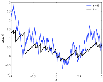
Figure 1: A snapshot of a Brownian initial velocity (thin line) and the corresponding solution to the Burgers equation at time one (thick line); notice the proliferation of shocks.

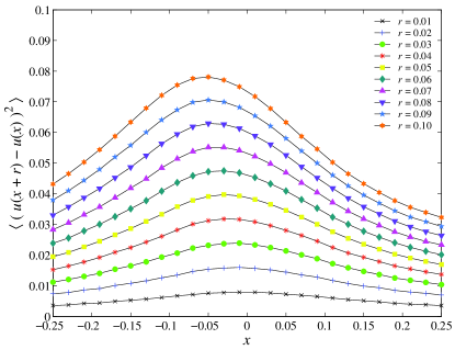
Figure 2: The second-order structure function for various separations $r$, plotted vs the absolute position $x$. Notice the strong $x$-dependence, evidence that incremental homogeneity does not hold. At large $x$ the graphs become flat (not shown).

A proof of the loss of incremental homogeneity in the temporal evolution from an initially incrementally homogeneous velocity can be given for the case of smooth initial data. The general idea is that as long as there are no shocks the solution can be Taylor expanded in time. The second-order structure function can then be calculated perturbatively and shown not to be translation-invariant. Actually for Gaussian initial data some of the realizations will develop shocks after very short times but their contribution to the structure function can be bounded by terms which are exponentially small in $1/t^{2}$. Because of its perturbative nature it is likely that the proof can be extended to the case of the 3-D Euler or Navier–Stokes equations. The proof is quite long and technical; its details do not belong here.

Since incrementally homogeneous random functions may be obtained by infrared limits of homogeneous random functions for which homogeneity persists under Burgers or Navier–Stokes dynamics, it is of interest to understand how homogeneity and incremental homogeneity are lost when the limit is taken. For concreteness we shall consider the Burgers equation with an initial velocity which is the Gaussian Ornstein–Uhlenbeck process (OUP). The argument given below is actually very general and can be applied mutatis mutandis to the Navier–Stokes equation. The OUP $u(x,0;k_{0})$ has the spectrum $1/(k_{0}^{2}+k^{2})$. Hence its correlation length $L\sim 1/k_{0}$ and its variance $\langle u^{2}(x,0;k_{0})\rangle\sim 1/k_{0}^{2}$ go to infinity as $k_{0}\to 0$. The Brownian motion process must be equal to zero at the origin. It is obtained from the OUP by first subtracting the random velocity $u(0,0;k_{0})$ and then letting $k_{0}\to 0$. We are here emphasizing “random” because there is a similar stress put by Kolmogorov on the first page of his first 1941 paper. It is clear that the effect of the initial subtraction of a uniform velocity will be a (random) Galilean transformation. Hence, denoting by $u(x,t;k_{0})$ the solution of the Burgers equation with the initial condition $u(x,0;k_{0})$, the solution of the problem with $u(0,0;k_{0})$ subtracted is

$$v(x,t;k_{0})\equiv u\left(x+tu(0,0;k_{0}),t;k_{0}\right)-u(0,0;k_{0}).$$ (3)

As $k_{0}\to 0$ the function $v(x,t;k_{0})$ tends to the solution with Brownian initial condition which was determined numerically above. Inspecting the r.h.s. of (3) we note that if we had only the subtraction of $u(0,0;k_{0})$ the solution and its limit would remain incrementally homogeneous. However, we also have a dependence on $u(0,0;k_{0})$ inside the spatial argument. Under the assumption of local homogeneity, the r.h.s. of (3) would be independent of the velocity $u(0,0;k_{0})$ at the reference point (here the origin) and thus $v$ would be incrementally homogeneous. It is this violation of local homogeneity (after subtraction of $u(0,0;k_{0})$) which spoils both homogeneity and incremental homogeneity. Local and incremental homogeneity can only hold in an asymptotic sense at points sufficiently remote in space-time from the reference point to be only weakly influenced by its velocity.

At the very beginning of his third 1941 turbulence paper on the four-fifths law Kolmogorovk41c assumed local homogeneity. How is the four-fifths law affected by what we just discussed? Monin and Yaglom my2 realized that there may be problems in deriving the four-fifths law (and its anisotropic generalization) using local homogeneity rather than full homogeneity. Hence they proposed first (on p. 395) to consider the locally homogeneous/isotropic turbulence as being embedded in a large-scale homogeneous turbulence. Then (on pp. 401–403) they derived the same results for locally homogeneous/isotropic turbulence using a quasi-Lagrangian method with a frame attached to a particular fluid particle. Actually, as we have seen, neither incremental nor local homogeneity can hold for turbulence which is initially not strictly homogeneous, except in an asymptotic sense which would not help in deriving a four-fifths law. Even in a putative incremental homogeneous turbulence, attempts to derive a four-fifths law lead to an extra non-vanishing term as shown in Ref. lindborg, (second term in Eq. (39)) and in Ref. hill02arxiv, (second term in Eq. (21)). This term is associated to the advection of products of two velocity differences by the half sum. Of course, the extra term vanishes if homogeneity (or local homogeneity) were to hold. We cannot rule out that some conditional form of homogeneity holds which allows a dependence on the reference velocity but is consistent with the four-fifths law.

When the turbulence is initially not homogeneous we cannot write a standard four-fifths law but there is still a relation between the local fluctuating energy dissipation $\varepsilon({\bm{x}})$ and the velocity increments, due to Duchon and Robert.dr00 In it simplest form it reads

$$\varepsilon(\bm{x})\!=\!\lim_{r\to 0}\frac{-3}{16\pi r^{2}}\!\!\int\!\!d\Omega\,|\bm{u}(\bm{x}+\bm{r})-\bm{u}(\bm{x})|^{2}(\bm{u}(\bm{x}+\bm{r})-\bm{u}(\bm{x}))\cdot\bm{r},$$ (4)

where $d\Omega$ is the element of solid angle spanned by the unit vector ${\bm{r}}/r$. This relation, which holds only after the limit $\nu\to 0$ has been taken, is between non-averaged quantities. In unpublished notes by Onsager (cited by Eyink and Sreenivasan es04 ) the same relation appears in averaged form. The Duchon–Robert formula is important because it is an exact consequence of the dynamical equations and also because it can be viewed as an infinitesimal version of Kolmogorov’s 1962 Refined Similarity Hypothesis.k62

We have seen that Kolomogorov’s assumption of independence of statistical properties of increments on the velocity at the reference point holds at best in an asymptotic sense, far from the reference point. More generally, one can ask if the small-scale properties of turbulent flow near a given point depend much on the instantaneous velocity $u_{0}$ at this point. There is good evidence that it does. For example, there are recent experimentalcmb04 and then numericalbbcdlt04 data showing a strong dependence of the variance of the fluid particle acceleration, conditioned on $u_{0}$, which is found to vary roughly as $u_{0}^{9/2}$. Indeed as shown in Ref. bbclt04, , large velocity and (extremely) large acceleration events occur in a correlated way near vortex filaments.

There is nothing surprising to find dependence on $u_{0}$ in homogeneous and isotropic turbulence: if in such a flow we observe a high fluctuation of the local velocity we also expect a high fluctuation in the local Reynolds number, a sharp decrease in the dissipation scale, etc. Some of the dependence on $u_{0}$ can be captured by adapting an old argument of Landau (see Ref. ufbook, Sec. 6.4.2). In its original form, Landau’s argument assumed that the mean dissipation $\varepsilon$ which appears in the Kolmogorov 1941 expression for the structure functions, can actually be taken as a quantity presenting large-scale fluctuations. As pointed out in Ref. frischshe91, arguments à la Landau have the potential of interlinking large-scale and small-scale phenomena. For this, one just uses the Kolmogorov 1941 predictions in terms of the large scale velocity $u_{0}$, the integral scale $L$ and the viscosity (when needed) and then one allows fluctuations in $u_{0}$. For example, as pointed out in Ref. am04, , from the Heisenberg–Yaglom theory which predicts that the typical acceleration of fluid particles is proportional to $u_{0}^{9/4}$, one can then infer that its conditional variance goes as $u_{0}^{9/2}$. If $u_{0}$ is assumed to have a Gaussian distribution, the PDF of the acceleration will involve a stretched exponential.bbcdlt04 Such non-Gaussianity should not be mistaken for intermittency. It is just a consequence of a slight extension of the Kolmogorov theory, which might be called Kolmogorov–Landau theory.

A delicate issue concerns the effect of $u_{0}$ on small-scale velocity increments and in particular on the longitudinal and transverse second-order structure functions. This question is now being revisited by various colleagues.

We are grateful to L. Biferale, E. Bodenschatz, G. Eyink, Y. Gagne, E. Lindborg, D. Mitra, J.-F. Pinton and K. Sreenivasan for useful remarks. This research was supported by the Indo-French Centre for the Promotion of Advanced Research (Project 2404-2), by the European Union under contract HPRN-CT-2002-00300 and by the Swedish Research Council under contract 2003-4614.

References

- (1) Kelvin, Lord (Sir W. Thomson), “On the propagation of laminar motion through a turbulently moving inviscid liquid,” Phil. Mag. 24, 342 (1887).
- (2) A.N. Shiryaev, “Kolmogorov and the turbulence”, available at www.maphysto.dk/publications/MPS-misc/1999/12.pdf .
- (3) A.N. Kolmogorov, “Curves in a Hilbert space that are invariant under the one-parameter group of motions,” Dokl. Akad. Nauk SSSR 26, 6 (1940).
- (4) A.N. Kolmogorov, “Wiener’s spiral and some interesting curves in Hilbert space,” Dokl. Akad. Nauk SSSR, 26, 115 (1940).
- (5) A.N. Kolmogorov, “The local structure of turbulence in incompressible viscous fluid for very large Reynolds number,” Dokl. Akad. Nauk SSSR 30, 9 (1940).
- (6) R.J. Hill, “Applicability of Kolmogorov’s and Monin’s equations of turbulence,” J. Fluid Mech. 353, 67 (1997).
- (7) R.J. Hill, “The approach of turbulence to the locally homogeneous asymptote as studied using exact structure-function equations”, arxiv:physics/0206034 (2002).
- (8) eds. A.S. Monin and A.M. Yaglom, Statistical Fluid Mechanics, vol. 2, ed. J. Lumley. MIT Press, Cambridge, MA (1975).
- (9) A.N. Kolmogorov, “Dissipation of energy in locally isotropic turbulence,” Dokl. Akad. Nauk SSSR 32, 16 (1941).
- (10) U. Frisch and J. Bec, “Burgulence”, in New Trends in Turbulence, A. Yaglom, F. David and M. Lesieur eds., Les Houches Session LXXIV (Springer EDP-Sciences, 2001) p. 341.
- (11) M. Vergassola, B. Dubrulle, U. Frisch and A. Noullez, “Burgers’ equation, Devil’s staircases and the mass distribution for large-scale structures, ”Astron. Astrophys. 289, 325 (1994).
- (12) Z.S. She, E. Aurell and U. Frisch, “The inviscid Burgers equation with initial conditions of Brownian type,” Comm. Math. Phys. 148, 623 (1992).
- (13) Ya. Sinai, “Statistics of shocks in solutions of inviscid Burgers equation,” Comm. Math. Phys. 148, 601 (1992).
- (14) E. Lindborg, “Horizontal velocity structure functions in the upper troposphere and lower stratosphere 2. Theoretical considerations,” J. Geophys. Res. 106, 10,233 (2001).
- (15) J. Duchon and R. Robert, “Inertial energy dissipation for weak solutions of incompressible Euler and Navier–Stokes equations,” Nonlinearity 13, 249 (2000).
- (16) G. Eyink and K. Sreenivasan, “Onsager and the theory of hydrodynamic turbulence,” Rev. Mod. Phys. in press (2005).
- (17) A.N. Kolmogorov, “A refinement of previous hypotheses concerning the local structure of turbulence in a viscous incompressible fluid at high Reynolds number,” J. Fluid Mech. 13, 82 (1962).
- (18) A.M. Crawford, N. Mordant and E. Bodenschatz, “Joint statistics of the Lagrangian acceleration and velocity in fully developed turbulence,” Phys. Rev. Lett. 94, 024501 (2005).
- (19) L. Biferale, G. Boffetta, A. Celani, B.J. Devenish, A. Lanotte and F. Toschi, “Multifractal statistics of Lagrangian velocity and acceleration in turbulence,” Phys. Rev. Lett. 93, 064502 (2004).
- (20) L. Biferale, G. Boffetta, A. Celani, A. Lanotte and F. Toschi, “Particle trapping in three-dimensional fully developed turbulence,” Phys. Fluids 17, 021701 (2005).
- (21) U. Frisch, Turbulence. The Legacy of A.N. Kolmogorov, Cambridge University Press, Cambridge (1995).
- (22) U. Frisch and Z.S. She, “On the probability density function of velocity gradients in fully developed turbulence,” Fluid Dyn. Res. 8, 139 (1991).
- (23) A.K. Aringazin and M.I. Mazhitov, “Stochastic models of Lagrangian acceleration of fluid particle in developed turbulence,” Int. J. Mod. Phys. B 18, 3095 (2004).